The Fractal Dimension of Interfaces in Edwards-Anderson and Long-range Ising Spin Glasses: Determining the Applicability of Different Theoretical Descriptions
Wenlong Wang, M. A. Moore, and Helmut G. Katzgraber

TL;DR
This study investigates the fractal dimension of interfaces in spin glasses across different dimensions using renormalization group methods, revealing the transition point where replica symmetry breaks and space-filling excitations emerge.
Contribution
It applies the strong-disorder renormalization group method to analyze the fractal dimension of domain walls in high-dimensional and long-range spin glasses, clarifying the applicability of theoretical models.
Findings
Replica symmetry breaks in high enough dimensions.
Space-filling excitations occur for dimensions 6 and above.
Results inform the appropriate theoretical description of spin glasses.
Abstract
The fractal dimension of excitations in glassy systems gives information on the critical dimension at which the droplet picture of spin glasses changes to a description based on replica symmetry breaking where the interfaces are space filling. Here, the fractal dimension of domain-wall interfaces is studied using the strong-disorder renormalization group method pioneered by Monthus [Fractals 23, 1550042 (2015)] both for the Edwards-Anderson spin-glass model in up to 8 space dimensions, as well as for the one-dimensional long-ranged Ising spin-glass with power-law interactions. Analyzing the fractal dimension of domain walls, we find that replica symmetry is broken in high-enough space dimensions. Because our results for high-dimensional hypercubic lattices are limited by their small size, we have also studied the behavior of the one-dimensional long-range Ising spin-glass with power-law…
Click any figure to enlarge with its caption.
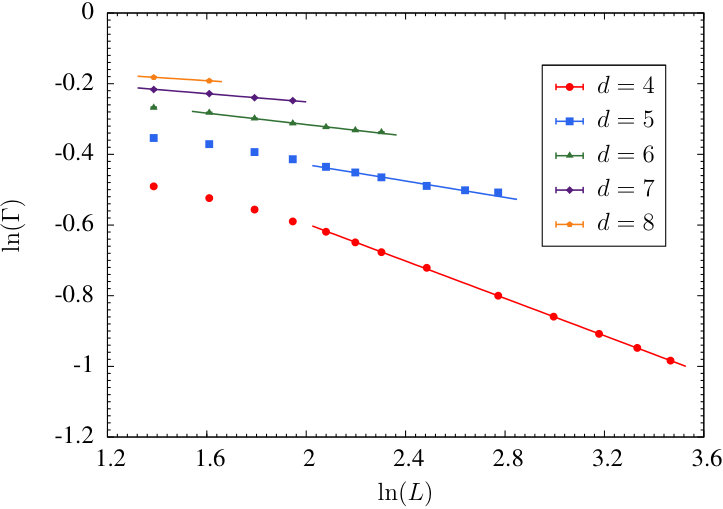 Figure 1
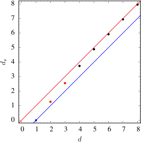 Figure 2
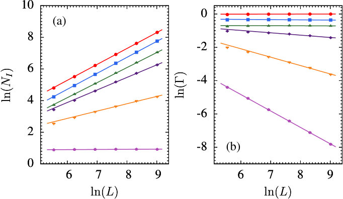 Figure 3
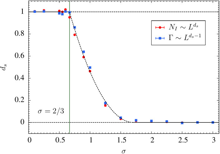 Figure 4
Peer Reviews
No public reviews on file for this paper yet. If you reviewed it on a platform where reviews are public (OpenReview, ICLR, NeurIPS, ICML), you can paste yours below so the community can read it here.
Videos
No videos yet. Explain this paper in a talk, walkthrough, or lecture? Add one.
Fractal Dimension of Interfaces in Edwards-Anderson and
Long-range Ising Spin Glasses:
Determining the Applicability of Different Theoretical Descriptions
Wenlong Wang
Department of Physics and Astronomy, Texas A&M University, College Station, Texas 77843-4242, USA
M. A. Moore
School of Physics and Astronomy, University of Manchester, Manchester M13 9PL, United Kingdom
Helmut G. Katzgraber
Department of Physics and Astronomy, Texas A&M University, College Station, Texas 77843-4242, USA
1QB Information Technologies (1QBit), Vancouver, British Columbia, Canada V6B 4W4
Santa Fe Institute, 1399 Hyde Park Road, Santa Fe, New Mexico 87501, USA
Abstract
The fractal dimension of excitations in glassy systems gives information on the critical dimension at which the droplet picture of spin glasses changes to a description based on replica symmetry breaking where the interfaces are space filling. Here, the fractal dimension of domain-wall interfaces is studied using the strong-disorder renormalization group method pioneered by Monthus [Fractals 23, 1550042 (2015)] both for the Edwards-Anderson spin-glass model in up to space dimensions, as well as for the one-dimensional long-ranged Ising spin-glass with power-law interactions. Analyzing the fractal dimension of domain walls, we find that replica symmetry is broken in high-enough space dimensions. Because our results for high-dimensional hypercubic lattices are limited by their small size, we have also studied the behavior of the one-dimensional long-range Ising spin-glass with power-law interactions. For the regime where the power of the decay of the spin-spin interactions with their separation distance corresponds to 6 and higher effective space dimensions, we find again the broken replica symmetry result of space filling excitations. This is not the case for smaller effective space dimensions. These results show that the dimensionality of the spin glass determines which theoretical description is appropriate. Our results will also be of relevance to the Gardner transition of structural glasses.
pacs:
75.50.Lk, 75.40.Cx, 05.50.+q
Spin glasses have been studied for more than half a century but there is still no consensus as to what order parameter describes their low-temperature phase. There are two competing theories: The oldest is the replica symmetry breaking (RSB) theory of Parisi Parisi (1979, 1983); Rammal et al. (1986); Mézard et al. (1987); Parisi (2008), which is known to be correct for the Sherrington-Kirkpatrick (SK) model Sherrington and Kirkpatrick (1975), which is the mean-field or infinite-dimensional limit of the short-range Edwards-Anderson (EA) Ising spin-glass model Edwards and Anderson (1975), the commonly used model for -dimensional systems. Within the RSB picture there are a very large number of pure states. In a second theory, known as the “droplet” picture McMillan (1984); Bray and Moore (1986); Fisher and Huse (1988) there are only two pure states and the low-temperature state is replica symmetric. In the droplet picture the behavior of the low-temperature phase is determined by low-lying excitations or droplets whose (free) energies scale in their linear extent as and whose interfaces have a fractal dimension . In the RSB theory, however, there exist low-lying excitations which cost an energy of and which are space filling, that is, . It has been argued Moore and Bray (2011) that when the droplet picture applies while for RSB is the appropriate picture. Note, however, that in finite space dimensions RSB is different from its infinite-dimensional limit; see Newman and Stein Newman and Stein (1998, 2001, 2002), as well as Read Read (2014) for details. In this paper we study the fractal dimension as a function of the space dimension, com , to find the space dimension at which the droplets become space-filling, i.e., when . Our results are consistent with being the critical dimension. It is, of course, difficult to overcome finite-size effects in numerical work near dimensions. Therefore, our main evidence that is the critical dimension comes from our study of the one-dimensional long-range spin-glass model introduced by Kotliar, Anderson and Stein (KAS) Kotliar et al. (1983). The calculational technique which we have used is the strong-disorder renormalization group (SDRG) introduced by Monthus Monthus (2015). This approach produces estimates of , that are in agreement with results on the EA model using other numerical techniques for space dimensions and (also studied by Monthus in Ref. Monthus (2015)). In this Letter, we extend the results of Ref. Monthus (2015) up to space dimensions, and apply the method introduced in the aforementioned reference to the KAS spin-glass model Kotliar et al. (1983).
Whether there is RSB or not in dimensions is not only important for spin glasses. In structural glasses there has been much recent interest in the Gardner transition, which is the transition at which replica symmetry breaking is supposed to occur to a glass state of marginal stability (for a review see Ref. Charbonneau et al. (2014)). However, recent numerical results have suggested that fluctuation effects about the mean-field solution might destroy the Gardner transition in at least space dimensions Scalliet et al. (2017). This result is entirely consistent with our expectation that replica symmetry breaking will be absent for .
The Edwards-Anderson model Edwards and Anderson (1975) is defined on a -dimensional cubic lattice of linear extent by the Hamiltonian
[TABLE]
where the summation is over only nearest-neighbor bonds and the random couplings are chosen from the standard Gaussian distribution of unit variance and zero mean. The Ising spins take the values with .
We have studied this model in space dimensions using the SDRG method Monthus (2015). Reference Monthus (2015) studied the cases of and . The SDRG approach successively traces out the spin whose orientation is most dominated by a single large renormalized bond to another spin; when the spin is eliminated the couplings of the remaining spins are renormalized accordingly. We refer the reader to Ref. Monthus (2015) for further details.
The observable we focus on is related to the bond average of , where is the number of bonds crossed by the domain wall when the boundary conditions in one direction are changed from periodic to antiperiodic. The SDRG method is essentially a way of constructing a possible ground state of the system. One runs the method twice, first with periodic and next with antiperiodic boundary conditions in one direction, and counts the bonds across which the relative spin orientation across the bond has altered because of the change of boundary conditions. Pictures of a domain wall so constructed for dimension can be found in Ref. Monthus (2015). It wanders, indicating that it has a fractal dimension and its length can be described by a fractal exponent , where . If the interface were straight across the system, its length would be proportional to . This means that because of the wandering one expects that . In the RSB phase the domain walls are space filling, i.e., . In general, .
We first introduce a more formal definition of which has a natural extension when we study long-range systems when the definition of an interface is far from obvious. One defines the link overlap Hartmann and Young (2002) via
[TABLE]
Here and denote the ground states found with periodic () and antiperiodic () boundary conditions, respectively. One can switch from periodic to antiperiodic boundary conditions by flipping the sign of the bonds crossing a hyperplane of the lattice. is the number of nearest-neighbor bonds in the lattice which for a -dimensional hypercube is given by . One can then define Hartmann and Young (2002)
[TABLE]
In Fig. 1 we show the bond-averaged value of [Eq. (3)] vs which should be a straight line of slope . In Fig. 2 the value of is plotted for various dimensionalities . For , (pentagon), while for we have used the value from Ref. Monthus (2015), i.e., (square), which is in excellent agreement with other numerical estimates Bray and Moore (1987); Middleton (2001); Hartmann and Young (2002); Melchert and Hartmann (2007); Amoruso et al. (2006); Bernard et al. (2007); Risau-Gusman and Romá (2008). For , Ref. Monthus (2015) quotes (square), which is again in good agreement with other estimates Palassini and Young (2000); Katzgraber et al. (2001). In addition, we estimate , which again is in good agreement with Monte Carlo estimates Katzgraber et al. (2001). Note that the largest system in Ref. Katzgraber et al. (2001) has spins, which seems to not be in the scaling regime (see Fig. 1). This means that results from small systems tend to overestimate .
Finally, one can see that as the dimensionality increases, approaches . However, results from simulations on hypercubic lattices struggle from corrections to scaling. These make it difficult to claim that at precisely . To address this point, we turn to the KAS model.
The one-dimensional KAS model Kotliar et al. (1983) is described by the Hamiltonian in Eq. (1), except that the spins lie on a ring and the exchange interactions are long ranged, i.e., denotes a sum over all pairs of spins:
[TABLE]
where is the shortest circular length between sites and Monthus (2014).
The disorder is chosen from a Gaussian distribution of zero mean and standard deviation unity, while the constant in Eq. (4) is fixed to make the mean-field transition temperature and , where represents a disorder average and where . Note that in the limit the KAS model reduces to the infinite-range SK model. The advantage of the KAS model is that one can study a large range of linear system sizes.
The KAS model can be taken as an interpolation between the EA model and the SK model as the exponent is varied. The phase diagram of this model in the – plane has been deduced from renormalization group arguments in Refs. Bray et al. (1986); Fisher and Huse (1988); Katzgraber and Young (2003a). For it behaves just like the infinite-range SK model. When the critical exponents at the spin-glass transition are mean-field like, and this corresponds in the EA model with space dimensions above . In the interval the critical exponents are changed by fluctuations away from their mean-field values. When , and when , the long-range zero-temperature fixed point, which controls the value of the exponents and , becomes identical to that of the nearest-neighbor one-dimensional EA model, i.e., and . There is a convenient mapping between and an effective dimensionality of the short-range EA model Katzgraber and Young (2003a); Katzgraber et al. (2009); Leuzzi et al. (2009); Baños et al. (2012); Aspelmeier et al. (2016a). For , it is
[TABLE]
Thus, right at the value of , . The arguments given in Ref. Moore and Bray (2011) that the critical dimension is , below which one sees droplet behavior and above which one sees RSB behavior were directly extended to the KAS model and predicted that only in the interval will one see RSB behavior, so that is the critical value expected for the KAS model.
We have determined for the KAS model from two definitions of . The first definition is via the generalization of the link overlap in Eq. (2) to the long-range KAS model just as done in Ref. Katzgraber and Young (2003b):
[TABLE]
where . Note that the sum of over equals . Antiperiodic boundary conditions can be produced by flipping the sign of the bonds when the shortest paths go through the origin. is then obtained from using Eq. (3) with .
Because we are unsure of the topological significance of calculated in this way, we use a second approach whose topological significance is clear. Fortunately, it gives very similar results to that of our first definition. Let , and define an “island” as a sequence in which all the are of the same sign. For the EA model limit of the KAS model, i.e., when , there are only two islands but when the long-range zero-temperature fixed point Bray et al. (1986) controls the behavior, there are many islands; we denote by the number of islands produced by the change from periodic to antiperiodic boundary conditions. Formally, can be computed via
[TABLE]
where . We define via . The islands have a distribution of sizes with their mean size . In the RSB region where is independent of the size of the system and is of , a result which we obtained previously from direct studies in the SK limit Aspelmeier et al. (2016b).
We have used these two quite distinct definitions of to compute the fractal dimension as a function of using the SDRG method. The details of the system sizes and numbers of disorder realizations can be found in Table 1. Our results for and are shown in Fig. 3. From these we have extracted values for which are shown in Fig. 4. The values obtained for from and are reassuringly similar. The most striking feature of our results are, first, when , and second, decreases from unity as increases past . Because maps to according to Eq. (5) we believe that this is strong evidence that is the dimension below which the droplet picture applies and that only in more than space dimensions will one find RSB effects, just as anticipated in Ref. Moore and Bray (2011).
At the long-range fixed point is unstable and the renormalization group flows go to the short-range fixed point, that of the EA model Bray et al. (1986). For the EA model in one space dimension, and . We were expecting that would go to zero at ; it is possible that is just very small in the interval .
There are small finite-size corrections when using the SDRG method. For , there is a downward curvature in the data (Fig. 3) so that if we had been able to study larger values, our estimates of might have decreased. However, the behavior in the crucial region where is close to is less affected by finite-size effects. Monthus and Garel Monthus and Garel (2014) have obtained estimates for from exact studies on the KAS model for . They found , , , , and . These results illustrate clearly that estimates of from small systems tend to be high.
We now discuss the accuracy of the SDRG method. First, we note that SDRG is considerably better than the Migdal-Kadanoff (MK) approximation which gives Monthus (2015), which coincides with the lower bound on and so never gives . The SDRG method can be used to determine as well as . In dimensions; it gives Monthus (2015); its established value is close to Hartmann et al. (2002). The SDRG method is only exact for special cases. Like the MK approximation, it is exact in one space dimension for the EA model but its performance for the energy per spin and the exponent then steadily deteriorates with increasing space dimension . Monthus Monthus (2015) suggested that it does a good job for the exponent because that exponent is dominated by short length-scale optimization which is well captured by the early steps of the SDRG method, but that it does badly for the interface free-energy exponent which also requires optimization on the longest length scales. We also suspect that its success in determining might be connected with the fact that the domain wall is a self-similar fractal. That means it has the same fractal dimension whether that fractal dimension is studied on short or long length scales. In and Monthus Monthus (2015) showed that the SDRG worked on short length scales but fails on long length scales. We believe the consequence of this might just be that in determining the length of the domain wall , the exponent is correctly determined from the short length-scale behavior, but to obtain the coefficient correctly one would need a treatment also valid on long length scales. In the KAS model at the SDRG fails on short length scales but works on long length scales. Again, we believe that the exponent is correct, but that the coefficient is only approximate.
One worrisome issue is that numerical work around space dimensions could suffer from poor precision, so how can one be confident that is a special space dimension below which RSB does not occur (aside from a rigorous proof). There is another numerical procedure, the greedy algorithm Cieplak et al. (1994); Newman and Stein (1994); Jackson and Read (2010); Sweeney and Middleton (2013) in which one satisfies the bonds in the order of the couplings unless a closed loop appears, where one skips to the next largest bond. We have found that as from below the values of obtained from the GA approach those from the SDRG, which is not surprising when one examines how the SDRG works. For , however, the GA is certainly poorer than the SDRG, because it predicts Sweeney and Middleton (2013). Jackson and Read Jackson and Read (2010), however, have an analytical argument that is a special space dimension for the GA algorithm. This gives us confidence that is the space dimension above which interfaces are space filling.
Acknowledgements.
W. W. and H. G. K. acknowledge support from NSF DMR Grant No. 1151387. The work of H.G.K. and W.W is supported in part by the Office of the Director of National Intelligence (ODNI), Intelligence Advanced Research Projects Activity (IARPA), via MIT Lincoln Laboratory Air Force Contract No. FA8721-05-C-0002. The views and conclusions contained herein are those of the authors and should not be interpreted as necessarily representing the official policies or endorsements, either expressed or implied, of ODNI, IARPA, or the U.S. government. The U.S. Government is authorized to reproduce and distribute reprints for Governmental purpose notwithstanding any copyright annotation thereon. We thank Texas A&M University for access to their Ada and Curie clusters.
The reference list from the paper itself. Each links out to its DOI / PubMed record.
- 1Parisi (1979) G. Parisi, “Infinite number of order parameters for spin-glasses,” Phys. Rev. Lett. 43 , 1754 (1979).
- 2Parisi (1983) G. Parisi, “Order parameter for spin-glasses,” Phys. Rev. Lett. 50 , 1946 (1983).
- 3Rammal et al. (1986) R. Rammal, G. Toulouse, and M. A. Virasoro, “Ultrametricity for physicists,” Rev. Mod. Phys. 58 , 765 (1986).
- 4Mézard et al. (1987) M. Mézard, G. Parisi, and M. A. Virasoro, Spin Glass Theory and Beyond (World Scientific, Singapore, 1987).
- 5Parisi (2008) G. Parisi, “Some considerations of finite dimensional spin glasses,” J. Phys. A 41 , 324002 (2008).
- 6Sherrington and Kirkpatrick (1975) D. Sherrington and S. Kirkpatrick, “Solvable model of a spin glass,” Phys. Rev. Lett. 35 , 1792 (1975).
- 7Edwards and Anderson (1975) S. F. Edwards and P. W. Anderson, “Theory of spin glasses,” J. Phys. F: Met. Phys. 5 , 965 (1975).
- 8Mc Millan (1984) W. L. Mc Millan, “Domain-wall renormalization-group study of the three-dimensional random Ising model,” Phys. Rev. B 30 , R 476 (1984).