Fast-slow asymptotic for semi-analytical ignition criteria in FitzHugh-Nagumo system
B. Bezekci, V. N. Biktashev

TL;DR
This paper develops an analytical approach to determine the initiation of excitation waves in the FitzHugh-Nagumo model, using singular perturbation theory with two small parameters to derive a closed-form strength-duration curve.
Contribution
It introduces a semi-analytical method employing singular perturbation with two small parameters to derive explicit ignition criteria in the FitzHugh-Nagumo system.
Findings
Derived analytical expressions for the boundary between resting and excited states.
Obtained a closed-form strength-duration curve for wave initiation.
Validated the analytical results with numerical simulations.
Abstract
We study the problem of initiation of excitation waves in the FitzHugh-Nagumo model. Our approach follows earlier works and is based on the idea of approximating the boundary between basins of attraction of propagating waves and of the resting state as the stable manifold of a critical solution. Here, we obtain analytical expressions for the essential ingredients of the theory by singular perturbation using two small parameters, the separation of time scales of the activator and inhibitor, and the threshold in the activator's kinetics. This results in a closed analytical expression for the strength-duration curve.
Click any figure to enlarge with its caption.
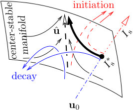 Figure 1
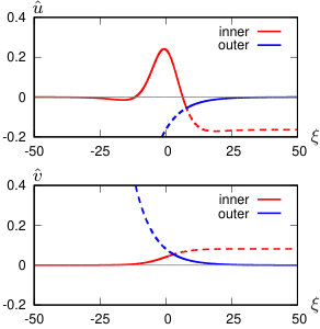 Figure 2
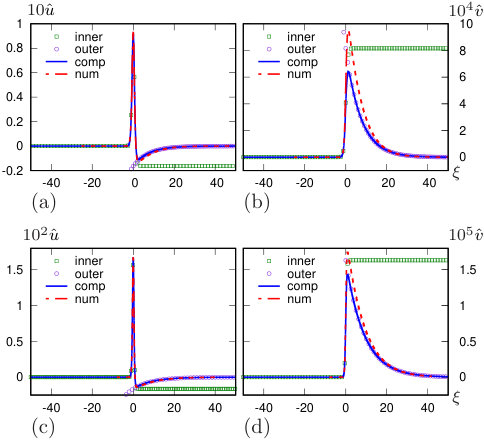 Figure 3
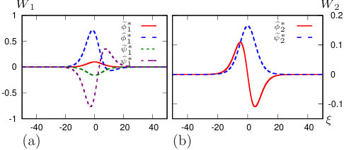 Figure 4
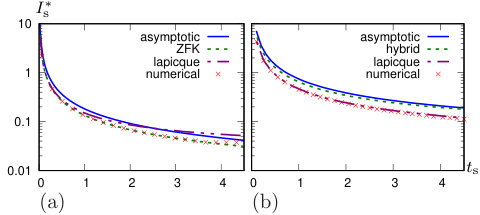 Figure 5
Peer Reviews
No public reviews on file for this paper yet. If you reviewed it on a platform where reviews are public (OpenReview, ICLR, NeurIPS, ICML), you can paste yours below so the community can read it here.
Videos
No videos yet. Explain this paper in a talk, walkthrough, or lecture? Add one.
\NewEnviron
eqsplit
[TABLE]
Fast-slow asymptotic for semi-analytical ignition
criteria in FitzHugh-Nagumo system
B. Bezekci
College of Engineering, Mathematics and Physical Sciences, University of Exeter, Exeter EX4 4QF, UK
V. N. Biktashev
College of Engineering, Mathematics and Physical Sciences, University of Exeter, Exeter EX4 4QF, UK
Abstract
We study the problem of initiation of excitation waves in the FitzHugh-Nagumo model. Our approach follows earlier works and is based on the idea of approximating the boundary between basins of attraction of propagating waves and of the resting state as the stable manifold of a critical solution. Here, we obtain analytical expressions for the essential ingredients of the theory by singular perturbation using two small parameters, the separation of time scales of the activator and inhibitor, and the threshold in the activator’s kinetics. This results in a closed analytical expression for the strength-duration curve.
Excitable reaction-diffusion systems underlie a large number of nontrivial spatio-temporal dynamic regimes and arise as models of a wide variety of physical, chemical and biological systems, some of which of considerable practical importance. One of such areas is electrophysiology of propagation of electric pulses in nerves and in the cardiac muscle. The detailed mathematical study of such models starts from Hodgkin and Huxley (1952). In their Nobel Prize work, they described how action potentials in neurons are initiated and propagated. Due to the complexity of a four-variable system, a particular attention has been devoted to obtain simpler and more mathematically tractable systems, one of which is FitzHugh-Nagumo model FitzHugh (1961); Fitzhugh (1960); Nagumo, Arimoto, and Yoshizawa (1962), widely accepted as an archetypical excitable model. Conditions of existence of propagating waves in such models and their properties is a subject of vast research literature. However, the question of conditions required to initiate such waves, or factors that may quench them, are no less important for applicationsBritton (1982); Zipes and Jalife (2000), and yet they are studied much less, because they are more complicated mathematically. The present paper is a part of an attempt to cover this gap, and endeavours to propose an analytical, albeit approximate, description of the initiation conditions, where previously only numerical treatment was believed possible.
I Introduction
Excitation waves may be defined as propagating nonlinear dissipative waves in a system which also possesses a spatially uniform resting state, stable with respect to small perturbations. Hence a transition from the resting state to a propagating wave requires a sufficiently large perturbation. The problem of what perturbations are sufficient to ignite an excitation wave is nonlinear, nonstationary, and generally lacks any helpful symmetries, thus generally is considered suitable only for numerical treatment. However, this problem has so many important applications that any analytical answers, even if only approximate and qualitative, are on high demand. One such analytical approach was investigated in our previous work Bezekci et al. (2015); Bezekci and Biktashev (2016). It is based on linearization of the dynamic equations around so-called critical solutions. These are unstable propagating waves (in some cases, stationary “nuclei”) which have exactly one unstable eigenvalue, so their centre-stable manifolds serve as boundaries separating the basins of attraction of the two possible outcomes, ignition (generation of the propagating wave) and failure (return to the resting state). This approach has demonstrated viability on some examples, but has a disadvantage in that the essential ingredients of the ignition criterion, such as the critical solution itself, as well as its leading eigenvalues and eigenfunctions, are to be obtained numerically. In this article, we focus particularly on the analytical initiation criterion in a spatially extended FitzHugh-Nagumo system, in which approximate propagating wave solutions are known in the limit of two small parameters, the ratio of the characteristic times of the activator and the inhibitor, and the threshold in the nonlinear kinetics of the activator. We use singular perturbation theory to construct the required ingredients for the linearized ignition criterion, and see how well the resulting criterion works.
The structure of the paper is as follows. In Section II, the analytical theory proposed in the earlier publications is summarized, with application to a two-component test problem, the FitzHugh-Nagumo model. The main contribution of this study is the analytical derivations of the essential ingredients of the threshold curves by means of the perturbation theory. Section III shows how these ingredients are obtained, along with the strength-duration curve approximation. Finally, in Section IV a short discussion of the results and some possible further research will be given.
II Theory
The FitzHugh-Nagumo model (FHN) may be presented in various equivalent forms. For this paper, we prefer the formulation used e.g. by Neu, Preissig, and Krassowska (1997):
[TABLE]
where {\color[rgb]{0,0,0}f}({\color[rgb]{0,0,0}u}) is a cubic polynomial function in the form {\color[rgb]{0,0,0}f}({\color[rgb]{0,0,0}u})={\color[rgb]{0,0,0}u}\left({\color[rgb]{0,0,0}u}-{\color[rgb]{0,0,0}\beta}\right)\left(1-{\color[rgb]{0,0,0}u}\right), the variables {\color[rgb]{0,0,0}u} and {\color[rgb]{0,0,0}v} represent respectively membrane potential and the recovery variables, {\color[rgb]{0,0,0}\gamma} is a small parameter describing the ratio of time scales of the variables {\color[rgb]{0,0,0}u} and {\color[rgb]{0,0,0}v}, and {\color[rgb]{0,0,0}\alpha} is a constant. The parameter {\color[rgb]{0,0,0}\beta} plays a key role in the fast dynamics of the model as it is the threshold state of the system that must be in the range in order for the system to have a qualitative electro-physiological meaning Maginu (1978, 1980).
In this paper, we consider the problem of initiation by a current pulse, modelled as a non-homogeneous Neumann boundary condition, with the rectangular profile of duration {\color[rgb]{0,0,0}{\color[rgb]{0,0,0}t}{\color[rgb]{0,0,0}{}_{\mathrm{s}}}} and strength of the current {\color[rgb]{0,0,0}I{\color[rgb]{0,0,0}{}_{\mathrm{s}}}},
[TABLE]
where is the Heaviside step function. Asymptotic behaviour of the solutions of excitable reaction-diffusion systems has been a topic of intense study, see for example Refs. [Aronson and Weinberger, 1975; McKean and Moll, 1985; Flores, 1989]. Typically, the solution of (2) either approaches the propagating pulse solution (“ignition”) or the resting state (“failure”). A curve in the ({\color[rgb]{0,0,0}{\color[rgb]{0,0,0}t}{\color[rgb]{0,0,0}{}_{\mathrm{s}}}},{\color[rgb]{0,0,0}I{\color[rgb]{0,0,0}{}_{\mathrm{s}}}})-plane that separates initial conditions leading to the ignition and initial conditions leading to the resting state is called a strength-duration curve. We shall also refer to it as a “threshold curve”, or “critical curve”.
The mathematical description of the threshold curve is motivated by the existence of a “critical solution”, which is an unstable relative equilibrium with a single unstable eigenvalue; for the FitzHugh-Nagumo system (2) it is a “critical pulse” Flores (1989, 1991); Idris and Biktashev (2008, 2007); Bezekci (2016). The stable manifold of such critical solution has codimension two, whereas its center-stable manifold has codimension one and as such, it can partition the phase space into two basins of attraction: one corresponds to the decay solutions, and the other to the initiation solutions, as sketched in Fig. 1. Of course, the concept of the “basin of attraction” is applicable to an autonomous problem, whereas our problem (2,3) is not. However, given a finite duration of the stimulating current, {\color[rgb]{0,0,0}{\color[rgb]{0,0,0}t}{\color[rgb]{0,0,0}{}_{\mathrm{s}}}}, we have an autonomous system for all {\color[rgb]{0,0,0}t}\geq{\color[rgb]{0,0,0}{\color[rgb]{0,0,0}t}{\color[rgb]{0,0,0}{}_{\mathrm{s}}}}, so the outcome of a stimulation will depend on which side of the centre-stable manifold will {\color[rgb]{0,0,0}\mathbf{u}}_{0}({\color[rgb]{0,0,0}x})={\color[rgb]{0,0,0}\mathbf{u}}({\color[rgb]{0,0,0}x},{\color[rgb]{0,0,0}{\color[rgb]{0,0,0}t}{\color[rgb]{0,0,0}{}_{\mathrm{s}}}}) be. This is further simplified by the fact that, even for a fixed {\color[rgb]{0,0,0}{\color[rgb]{0,0,0}t}{\color[rgb]{0,0,0}{}_{\mathrm{s}}}}, we have a one-parameter family of such initial conditions, depending on the parameter {\color[rgb]{0,0,0}I{\color[rgb]{0,0,0}{}_{\mathrm{s}}}}. This will correspond to a curve {\color[rgb]{0,0,0}\mathbf{u}}_{0}({\color[rgb]{0,0,0}x};{\color[rgb]{0,0,0}I{\color[rgb]{0,0,0}{}_{\mathrm{s}}}}) in the functional space (dash-dotted line in fig. 1). The critical value {\color[rgb]{0,0,0}I_{\mathrm{s}}^{*}}, corresponding to the boundary between failure and success, corresponds to the point of intersection between this curve and the centre-stable manifold (bold filled circle). By construction, the initial protocol corresponding to the intersection point, produces a trajectory (bold arrow) that lies on the boundary of the basins, i.e. is a “saddle straddle trajectory” in the terminology of Ref. [Nusse and Yorke, 1989], and approaches the unstable solution {\color[rgb]{0,0,0}\hat{{\color[rgb]{0,0,0}\mathbf{u}}}} (dashed arrow) as {\color[rgb]{0,0,0}t}\to\infty.
Analytical expressions for the ignition criteria can be obtained by approximating this center-stable manifold by its tangent at the critical solution, i.e. the center-stable space; the feasibility of quadratic approximation was also demonstrated in some cases. Details of this approach have been described elsewhereBezekci et al. (2015); Bezekci and Biktashev (2016), and here we only quote the required results. The primary ingredient for the theory is of course the critical solution itself, which for the FHN system has the form of the critical pulse {\color[rgb]{0,0,0}\mathbf{u}}({\color[rgb]{0,0,0}x},{\color[rgb]{0,0,0}t})={\color[rgb]{0,0,0}\hat{{\color[rgb]{0,0,0}\mathbf{u}}}}({\color[rgb]{0,0,0}\xi})=\begin{pmatrix}{\color[rgb]{0,0,0}\hat{{\color[rgb]{0,0,0}u}}}({\color[rgb]{0,0,0}\xi}),{\color[rgb]{0,0,0}\hat{{\color[rgb]{0,0,0}v}}}({\color[rgb]{0,0,0}\xi})\end{pmatrix}^{T}, where {\color[rgb]{0,0,0}\xi}={\color[rgb]{0,0,0}x}-{\color[rgb]{0,0,0}c}{\color[rgb]{0,0,0}t}-{\color[rgb]{0,0,0}s}, the constant (nonlinear eigenvalue) {\color[rgb]{0,0,0}c} is the speed of the critical pulse, and {\color[rgb]{0,0,0}s}\in\mathbb{R} is an arbitrary constant. Beyond that, the theory requires two leading left eigenfunctions {\color[rgb]{0,0,0}\mathbf{W}_{1}}=\begin{pmatrix}{\color[rgb]{0,0,0}\phi^{*}_{1}},{\color[rgb]{0,0,0}\psi^{*}_{1}}\end{pmatrix}^{T}, {\color[rgb]{0,0,0}\mathbf{W}_{2}}=\begin{pmatrix}{\color[rgb]{0,0,0}\phi^{*}_{2}},{\color[rgb]{0,0,0}\psi^{*}_{2}}\end{pmatrix}^{T} and first leading eigenvalue {\color[rgb]{0,0,0}\lambda_{1}}; note that {\color[rgb]{0,0,0}\lambda_{2}}=0, due to the translational symmetry. The ignition criterion has been formulated as a finite nonlinear system of two equations for two unknowns, {\color[rgb]{0,0,0}s} and {\color[rgb]{0,0,0}I{\color[rgb]{0,0,0}{}_{\mathrm{s}}}},
[TABLE]
where the right-hand sides {\color[rgb]{0,0,0}\mathcal{N}_{1}} and {\color[rgb]{0,0,0}\mathcal{N}_{2}} are constants, defined entirely by the properties of the model,
[TABLE]
Here and below, we use the bra-ket notation for the inner product: if and , then
[TABLE]
The compatibility condition for the two equations given in (4) for {\color[rgb]{0,0,0}I{\color[rgb]{0,0,0}{}_{\mathrm{s}}}} is
[TABLE]
In the previous works, we have been unable to find any ingredients in these formulations required for the definition of strength-duration threshold curve analytically with a few exceptions of limited practical importance. Hence, a hybrid approach where these key ingredients are determined numerically must typically be employed. In the present paper, we obtain the required ingredients analytically, which will allow description of the strength-duration curve in a closed analytical form. This is achieved by using perturbation theory with {\color[rgb]{0,0,0}\gamma} and {\color[rgb]{0,0,0}\beta} as small parameters.
III Perturbation Analysis
In this section, we employ the perturbation theory to obtain the critical pulse and leading eigenfunctions and corresponding eigenvalues of FHN system using the exact solution of its fast subsystem, Zeldovich-Frank-Kamenetsky (ZFK) equation, sometimes also called Nagumo equation:
[TABLE]
Clearly, when we set {\color[rgb]{0,0,0}\gamma}=0 and {\color[rgb]{0,0,0}v}\equiv 0, FHN system transforms into ZFK equation and formally, we use a series in {\color[rgb]{0,0,0}\gamma} and the solution of ZFK equation to have the approximation to the full solution of FHN system.
III.1 Finding the critical pulse
To find the critical pulse, we look for solutions of the form {\color[rgb]{0,0,0}u}({\color[rgb]{0,0,0}x},{\color[rgb]{0,0,0}t})={\color[rgb]{0,0,0}\hat{{\color[rgb]{0,0,0}u}}}({\color[rgb]{0,0,0}\xi}), {\color[rgb]{0,0,0}v}({\color[rgb]{0,0,0}x},{\color[rgb]{0,0,0}t})={\color[rgb]{0,0,0}\hat{{\color[rgb]{0,0,0}v}}}({\color[rgb]{0,0,0}\xi}) where {\color[rgb]{0,0,0}\xi}={\color[rgb]{0,0,0}x}-{\color[rgb]{0,0,0}c}{\color[rgb]{0,0,0}t}, and the positive constant {\color[rgb]{0,0,0}c} is the propagation speed of the rightward traveling wave, yet to be determined. Then, the FHN system is converted into following system of first order ordinary differential equations:
[TABLE]
The traveling wave solution vanishes at both infinities along with its first derivative
[TABLE]
Hastings (1976) has proved that for a sufficiently small {\color[rgb]{0,0,0}\gamma}, there are at least two distinct positive numbers {\color[rgb]{0,0,0}c} such that the above system has a homoclinic. It was also proved that the higher speed is {\color[rgb]{0,0,0}c}\left({\color[rgb]{0,0,0}\gamma}\right)\approx\sqrt{2}\left(\frac{1}{2}-{\color[rgb]{0,0,0}\gamma}\right) and the corresponding pulse is stable, while the slower speed is {\color[rgb]{0,0,0}c}\left({\color[rgb]{0,0,0}\gamma}\right)=\mathcal{O}\!\left(\sqrt{{\color[rgb]{0,0,0}\gamma}}\right) and the slower pulse is unstable, with one positive eigenvalue Flores (1991); Hastings (1982). That is, the slow pulse is our critical pulse, and we restrict our analysis to it. We use the matching asymptotics method: divide the domain of the problem into two subdomains: the inner region where the solution changes rapidly ((with a speed ) in the limit {\color[rgb]{0,0,0}\gamma}\searrow 0, and the outer solution where it varies slowly (with a speed \mathcal{O}\!\left({\color[rgb]{0,0,0}\gamma}^{1/2}\right)). The solutions obtained in these regions are called as inner and outer solutions, respectively. The inner and outer solutions are then matched to ensure that the approximate solution is uniformly valid in the whole domain. This is achieved by using a transition zone, in which the two solutions are asymptotically equal.
III.1.1 Inner Expansion
Following Ref. [Casten, Cohen, and Lagerstrom, 1975], we represent the inner asymptotics of the solution in the form
[TABLE]
where {\color[rgb]{0,0,0}\tilde{\color[rgb]{0,0,0}v}_{0}}\equiv 0 and {\color[rgb]{0,0,0}{\color[rgb]{0,0,0}c}_{0}}=0 as the ZFK equation is one-component and its critical nucleus solution has zero velocity. Substituting these into equation (8) and collecting the terms by the powers of {\color[rgb]{0,0,0}\gamma}^{1/2}, we have
[TABLE]
Coefficient {\color[rgb]{0,0,0}{\color[rgb]{0,0,0}c}_{1}} can be determined by multiplying (12) by \mathrm{d}{\color[rgb]{0,0,0}\tilde{\color[rgb]{0,0,0}u}_{0}}/\mathrm{d}{\color[rgb]{0,0,0}\xi} and then integrating the result using the equations (11) and (13) therein, giving
[TABLE]
where the integration is performed over the inner domain. As we aim to obtain explicit analytical expressions as much as possible, we consider the limit of small {\color[rgb]{0,0,0}\beta}. For {\color[rgb]{0,0,0}u}\lesssim{\color[rgb]{0,0,0}\beta} we can approximate {\color[rgb]{0,0,0}f}({\color[rgb]{0,0,0}u})\approx{\color[rgb]{0,0,0}u}\left({\color[rgb]{0,0,0}u}-{\color[rgb]{0,0,0}\beta}\right) for which the critical nucleus of ZFK isIdris and Biktashev (2008); Neu, Preissig, and Krassowska (1997)
[TABLE]
so that the speed correction evaluates to
[TABLE]
Equation (13) for {\color[rgb]{0,0,0}\tilde{\color[rgb]{0,0,0}v}_{1}} is first order separable, and its solution satisfying {\color[rgb]{0,0,0}\tilde{\color[rgb]{0,0,0}v}_{1}}(-\infty)=0 is
[TABLE]
Equation (12) for {\color[rgb]{0,0,0}\tilde{\color[rgb]{0,0,0}u}_{1}} is second order linear and we know that \mathrm{d}{\color[rgb]{0,0,0}\tilde{\color[rgb]{0,0,0}u}_{0}}/\mathrm{d}{\color[rgb]{0,0,0}\xi} is a solution, so its general solution can be found by the substitution
[TABLE]
which gives a first-order linear equation for {\color[rgb]{0,0,0}p}, leading to
[TABLE]
III.1.2 Outer Expansion
Technically, we have two outer regions, for {\color[rgb]{0,0,0}\xi}<0 and {\color[rgb]{0,0,0}\xi}>0. The inner solution obtained above satisfies the boundary conditions at {\color[rgb]{0,0,0}\xi}\to-\infty, but not at {\color[rgb]{0,0,0}\xi}\to\infty. Hence the outer solution for {\color[rgb]{0,0,0}\xi}<0 may be taken as zero both for {\color[rgb]{0,0,0}u} and {\color[rgb]{0,0,0}v}, whereas for {\color[rgb]{0,0,0}\xi}>0 a nontrivial solution must be found. There, we use the independent variable {\color[rgb]{0,0,0}\zeta}={\color[rgb]{0,0,0}\gamma}^{1/2}{\color[rgb]{0,0,0}\xi}, and assume the solution in the form of a power series in {\color[rgb]{0,0,0}\gamma}^{1/2}, starting with
[TABLE]
Substituting these into (8) and collecting the terms by the powers of {\color[rgb]{0,0,0}\gamma}^{1/2}, we get
[TABLE]
which have the following nontrivial solutions
[TABLE]
where the constant {\color[rgb]{0,0,0}A} is to be determined from the condition that the inner and outer expansions give the same result in the transition zone. This can be achieved by applying the Van Dyke’s matching principle Van Dyke (1975), requiring that the inner solution in the transition zone (i.e. as {\color[rgb]{0,0,0}\xi}\to\infty) is equal to the outer solution in the transition zone (i.e. as {\color[rgb]{0,0,0}\zeta}\to 0):
[TABLE]
which gives
[TABLE]
Fig. 2 shows the inner and outer solutions of {\color[rgb]{0,0,0}\hat{{\color[rgb]{0,0,0}u}}} and {\color[rgb]{0,0,0}\hat{{\color[rgb]{0,0,0}v}}} components of the critical pulse for the FHN system for the parameter values, {\color[rgb]{0,0,0}\gamma}=0.01, {\color[rgb]{0,0,0}\beta}=0.05, {\color[rgb]{0,0,0}\alpha}=0.37. In the negative {\color[rgb]{0,0,0}\xi} region, the inner solution is uniformly valid. In the positive {\color[rgb]{0,0,0}\xi} region, on the other hand, neither the inner nor the outer solutions alone can be the solution and we would like to combine these two solutions into a “composite solution” that would be uniformly valid. This can be done by adding the inner and outer approximations and subtracting the matching value, which would have been taken into account twice otherwise. Thus, our final critical pulse solution based on perturbation theory, valid in the whole domain, is in the following form,
[TABLE]
where the matching values are
[TABLE]
and we have dropped the terms \mathcal{O}\!\left({\color[rgb]{0,0,0}\gamma}\right) throughout.
Fig. 3 shows the critical pulse solutions of FHN system based on the asymptotic perturbation theory analysis compared with the ones obtained numerically. We used the numerical methods described in Ref. [Bezekci et al., 2015]. The figure illustrates two selected set of parameters, {\color[rgb]{0,0,0}\gamma}=0.001, {\color[rgb]{0,0,0}\beta}=0.05, {\color[rgb]{0,0,0}\alpha}=0.37 (top panel) and {\color[rgb]{0,0,0}\gamma}=0.00001, {\color[rgb]{0,0,0}\beta}=0.01, {\color[rgb]{0,0,0}\alpha}=0.37 (bottom panel). It can be seen that the asymptotic result gets closer to the numerical critical pulse when the parameters {\color[rgb]{0,0,0}\beta} and {\color[rgb]{0,0,0}\gamma} both become smaller, which is indeed expected.
III.2 Finding the Leading Eigenvalues and Eigenfunctions
In a similar fashion, perturbation theory can be applied to approximate the eigenfunctions and eigenvalues of FHN system. Generally speaking, the eigenvalue problem is to be solved by matching asymptotics as well. However, in our case the inner solution happens to vanish at both infinities so both outer solutions can be taken as zero, and we only need to look at the inner solution.
To begin with, we linearize the FHN system (2) around the critical pulse in the co-moving frame of reference {\color[rgb]{0,0,0}\xi}={\color[rgb]{0,0,0}x}-{\color[rgb]{0,0,0}c}{\color[rgb]{0,0,0}t}, {\color[rgb]{0,0,0}\tau}={\color[rgb]{0,0,0}t},
[TABLE]
such that FHN system with quadratic nonlinearity gives
[TABLE]
We are looking for solutions of the linearized problem of the form {\color[rgb]{0,0,0}U}\left({\color[rgb]{0,0,0}\xi},{\color[rgb]{0,0,0}t}\right)=\mathrm{e}^{{\color[rgb]{0,0,0}\lambda}{\color[rgb]{0,0,0}\tau}}{\color[rgb]{0,0,0}\phi}({\color[rgb]{0,0,0}\xi}) and {\color[rgb]{0,0,0}V}\left({\color[rgb]{0,0,0}\xi},{\color[rgb]{0,0,0}\tau}\right)=\mathrm{e}^{{\color[rgb]{0,0,0}\lambda}{\color[rgb]{0,0,0}\tau}}{\color[rgb]{0,0,0}\psi}({\color[rgb]{0,0,0}\xi}), which leads to the right eigenfunction problem,
[TABLE]
where
[TABLE]
Inserting the speed and critical pulse defined in the inner expansion analysis into the operator {\color[rgb]{0,0,0}\mathcal{L}}, we have
[TABLE]
where
[TABLE]
Now, we expand the eigenvalues and eigenfunctions in a power series in terms of {\color[rgb]{0,0,0}\gamma}^{1/2},
[TABLE]
This kind of expansion has been widely used in the field of quantum mechanics, see for example Ref. [Sakurai and Napolitano, 2011]. Implementing this eigenpair expansion into the original eigenvalue problem (25), we have
[TABLE]
Equating this in terms of the coefficients of the powers of {\color[rgb]{0,0,0}\gamma}^{1/2}, we get
[TABLE]
for {\color[rgb]{0,0,0}j}=1,2,\ldots. The leading order equation (26) reduces to the eigenvalue problem of the unperturbed problem, ZFK equation, and the leading eigenpair for it is known explicitly Idris and Biktashev (2008):
[TABLE]
Also, due to the translational symmetry, the second eigenpair is delivered by the derivative of the critical nucleus solution of the ZFK equation,
[TABLE]
As discussed in Section II, the linearized ignition criterion requires knowledge of solutions of the adjoint linearized problem
[TABLE]
where in our case
[TABLE]
We write
[TABLE]
where
[TABLE]
We look for the left eigenfunctions in the form of asymptotic series as
[TABLE]
and the series for the eigenvalues the same as for the right eigenfunctions. Inserting these series into (29) and balancing the terms up to the order of {\color[rgb]{0,0,0}\gamma}^{1/2}, we have
[TABLE]
The leading order equation (30) gives straightforwardly
[TABLE]
Our next goal is to find the eigenvalue perturbations. We rewrite (27) as
[TABLE]
We already know the leading order for {\color[rgb]{0,0,0}j}=1,2. Now we take the inner product of the left-hand side of (32) with {\color[rgb]{0,0,0}\widetilde{\mathbf{W}}_{{\color[rgb]{0,0,0}j}}} to get
[TABLE]
since {\color[rgb]{0,0,0}\widetilde{\mathbf{W}}_{{\color[rgb]{0,0,0}j}}} is an eigenfunction of {\color[rgb]{0,0,0}{\color[rgb]{0,0,0}\mathcal{L}}^{+}_{0}} and the inner product is semilinear in the first factor. Using this result in (27), we obtain the classical expression for the eigenvalue perturbations,
[TABLE]
In particular, for {\color[rgb]{0,0,0}j}=1, we find the leading eigenvalue as
[TABLE]
and we of course have
[TABLE]
due to the translational symmetry.
The linear approximations of the critical curves require the knowledge of the left eigenfunctions, i.e. the eigenfunctions of the adjoint linearized equation. Hence, we skip the details of the analytical construction of the right eigenfunctions and proceed straight to finding the left eigenfunctions perturbations, {\color[rgb]{0,0,0}\widehat{\mathbf{W}}_{{\color[rgb]{0,0,0}j}}}. We begin with the first component of the {\color[rgb]{0,0,0}j}=1 left eigenfunction. It satisfies
[TABLE]
or
[TABLE]
where
[TABLE]
We know one solution of the corresponding homogeneous equation, {\color[rgb]{0,0,0}R}({\color[rgb]{0,0,0}\xi})=0, which is {\color[rgb]{0,0,0}\widetilde{\phi}^{*}_{1}}=\mathrm{sech}^{3}\left({\color[rgb]{0,0,0}\xi}\sqrt{{\color[rgb]{0,0,0}\beta}}/2\right). So we look for the solution of the full non-homogeneous equation using the reduction-of-order substitution
[TABLE]
leading to
[TABLE]
The general solution of this is
[TABLE]
where {\color[rgb]{0,0,0}C_{1}} and {\color[rgb]{0,0,0}C_{2}} are constants of the integration. The resulting explicit expression for {\color[rgb]{0,0,0}\widehat{\phi}_{1}^{*}} is
[TABLE]
where
[TABLE]
Remember that the inner solution for the critical nucleus is uniformly valid for {\color[rgb]{0,0,0}\xi}<0. Hence we expect the inner solutions for the eigenfunctions also to be uniformly valid for {\color[rgb]{0,0,0}\xi}<0. In particular, they should be bounded at {\color[rgb]{0,0,0}\xi}\to-\infty. We have
[TABLE]
Consequently, the constant {\color[rgb]{0,0,0}C_{1}} must be zero. Then (37) simplifies to
[TABLE]
Before we can find the constant {\color[rgb]{0,0,0}C_{2}}, we need to find also the second component of the first adjoint eigenfunction; this is easily found as
[TABLE]
The value of the constant {\color[rgb]{0,0,0}C_{2}} can then be found from the orthogonality condition \left\langle{\color[rgb]{0,0,0}\mathbf{W}_{1}}\,\Big{|}\,{\color[rgb]{0,0,0}\mathbf{V}_{2}}\right\rangle=0. In the expanded form, this can be written as
[TABLE]
where the first term vanishes due to (28) as \begin{pmatrix}{\color[rgb]{0,0,0}\tilde{\color[rgb]{0,0,0}u}_{0}}^{\prime},&0\end{pmatrix}^{T} is the {\color[rgb]{0,0,0}j}=2 right eigenfuntion so automatically is orthogonal to \begin{pmatrix}{\color[rgb]{0,0,0}\widetilde{\phi}^{*}_{1}},{\color[rgb]{0,0,0}\widetilde{\psi}^{*}_{1}}\end{pmatrix}^{T}. Similarly, the second term in the above formula also vanishes since the sum of all three definite integrals is equal to zero as calculated below,
[TABLE]
(the integral multiplied by {\color[rgb]{0,0,0}C_{2}} here vanishes as it is the same as the one discussed above),
[TABLE]
[TABLE]
Therefore, the constant {\color[rgb]{0,0,0}C_{2}} can be found from the third term, giving
[TABLE]
Conceivably, the integrals here can be evaluated analytically, but the results would be too complicated so in the illustrations presented below, we have just done it numerically (remember that these are definite integrals, so for fixed parameter values these are just constants). Finding {\color[rgb]{0,0,0}C_{2}} completes the derivation of {\color[rgb]{0,0,0}\mathbf{W}_{1}}.
For {\color[rgb]{0,0,0}\mathbf{W}_{2}}, the formulas (39) and (40) above do not work as {\color[rgb]{0,0,0}\lambda_{2}}=0. Instead, we use the following expansion:
[TABLE]
Substituting this into the left eigenfunction equation (29) and balancing the powers of {\color[rgb]{0,0,0}\gamma}^{1/2}, we have
[TABLE]
with solutions
[TABLE]
Fig. 4 shows the asymptotic components of the first two eigenfunctions of FHN system for the parameters {\color[rgb]{0,0,0}\beta}=0.05, {\color[rgb]{0,0,0}\alpha}=0.37. The eigenfunctions vanish at {\color[rgb]{0,0,0}\xi}\to-\infty by construction; however, the result of our calculations is that they also vanish at {\color[rgb]{0,0,0}\xi}\to\infty, hence it is not necessary to consider the outer expansion for them.
III.3 Strength-Duration Curve
After finding the asymptotics of the eigenfunctions of the model in closed forms, we can use those to construct the approximation to the critical curves. In this paper, we restrict consideration to the strength-duration curve.
In our proposed procedure, the value of {\color[rgb]{0,0,0}s} is given by the transcendental equation (6). Employing the found asymptotics, we obtain
[TABLE]
The integral {\color[rgb]{0,0,0}I_{3}} in this equation is calculated as
[TABLE]
where
[TABLE]
and is the Lerch transcendent, defined e.g. in Ref. [Bateman et al., 1955] as
[TABLE]
provided that |{\color[rgb]{0,0,0}z}|<1 and {\color[rgb]{0,0,0}q}\neq 0,-1,\ldots.
The integral {\color[rgb]{0,0,0}I_{4}} is also calculated as a function of the Lerch transcendent as
[TABLE]
where
[TABLE]
and finally the integral {\color[rgb]{0,0,0}I_{5}} is calculated as
[TABLE]
A further simplification can be achieved by taking into account that {\color[rgb]{0,0,0}\beta} is also a small parameter. With a substitution {\color[rgb]{0,0,0}\rho}=\mathrm{e}^{{\color[rgb]{0,0,0}\xi}\sqrt{{\color[rgb]{0,0,0}\beta}}}, the limits of all three integrals become close to . Hence, these integrals can be evaluated as the Taylor expansion around and they become regular functions,
[TABLE]
[TABLE]
[TABLE]
Plugging these back into the transcendental equation (III.3), we have
[TABLE]
and equating this up to the order of {\color[rgb]{0,0,0}\gamma}^{1/2} gives the value of {\color[rgb]{0,0,0}s} as
[TABLE]
Having obtained a closed expression for {\color[rgb]{0,0,0}s}, the final step is to substitute this into one of the equations in (4), which finally delivers the formula for the strength-duration curve:
[TABLE]
The plots of the asymptotic threshold curves given by equation (45), compared against the direct numerical simulations, are shown in Fig. 5. The left panel of the figure shows the case of a very small {\color[rgb]{0,0,0}\gamma}, and we show also the numerical curve for ZFK equation, i.e. the {\color[rgb]{0,0,0}\gamma}\to 0 limit of FHN. We observe that there is a good agreement between the two numerical curves. In the right panel of the figure, the values of both {\color[rgb]{0,0,0}\gamma} and {\color[rgb]{0,0,0}\beta} are increased compared to the left panel. Here instead of the ZFK curve, we show the “hybrid” numeric-asymptotic prediction, that is, the asymptotic result given by linearized theory (4,5,6), in which the ingredients {\color[rgb]{0,0,0}\hat{{\color[rgb]{0,0,0}\mathbf{u}}}}, {\color[rgb]{0,0,0}\mathbf{W}_{1,2}} and {\color[rgb]{0,0,0}\lambda_{1}} are found numerically using methods described in Ref. [Bezekci et al., 2015]. The closeness of the asymptotic curve to the hybrid curve in this panel, despite the fact that {\color[rgb]{0,0,0}\gamma} and {\color[rgb]{0,0,0}\beta} are not very small, is an illustration of the quality of the asymptotic formulas for the said ingredients, which is the main technical result of this paper. Expectedly, the asymptotic threshold curve, in this case, is not better than the hybrid prediction.
Out of curiosity, for each figure we also plot the curves described by the equation
[TABLE]
which is the classical formula going back to works by Lapicque (1907), Blair (1932) and Hill (1936) as a phenomenological law approximating excitation thresholds in a wide range of electrophysiological experiments, well before the realistic models of any biological excitable tissues became available. For theoretical justification, already Lapicque (1907) proposed a hypothetical linear electric circuit that can produce this dependence; nowadays this may be considered as a linearization of actual nonlinear membrane equations. In the spatially extended context, it has been shownIdris and Biktashev (2008) that (46) automatically emerges as a result of the linearized theory (4,5,6) in the case of “critical nucleus”, {\color[rgb]{0,0,0}c}=0, {\color[rgb]{0,0,0}s}=0, regardless of other details of the model. In fig. 5, the values of the rheobase {\color[rgb]{0,0,0}I_{rh}} and chronaxie {\color[rgb]{0,0,0}\tau} are not obtained theoretically, but fitted to the numerical curves using the Levenberg-Marquardt nonlinear least-squares fitting algorithm Levenberg (1944); Marquardt (1963). We note that the Lapicque-Blair-Hill curve fits the results of direct simulations much better for the right panel, even though the theoryIdris and Biktashev (2008) promises its applicability to the case {\color[rgb]{0,0,0}\gamma}=0, which is closer to the case in the left panel. The reasons for this paradoxical discrepancy, apart from the simple fact that the analytical formula is only approximate in any case, are not clear at present and require further investigation.
IV Discussion
The semi-analytical approach to the strength-extent and strength-duration threshold curves has been presented in our previous publicationsBezekci et al. (2015); Bezekci and Biktashev (2016). In the multicomponent reaction-diffusion systems, the essential ingredients for the case of the strength-extent curve are moving critical solution (either critical front or critical pulse) and two leading left (adjoint) eigenfunctions, whereas for the case of the strength-duration curve, we additionally need the positive eigenvalue {\color[rgb]{0,0,0}\lambda_{1}}. In Refs. [Bezekci et al., 2015] and [Bezekci and Biktashev, 2016], the case of FitzHugh-Nagumo was considered among others, and these ingredients were found only numerically, which of course depreciated the heuristical value of the results, not to speak of associated computational cost and numerical analyst’s effort.
The main aim of this article has been to overcome this disadvantage to approximately calculate the analytical expressions for the ingredients of the FHN theory and obtain a closed-form expression for the critical curve. As FHN system is considered as a ZFK equation extended by a slow variable and all essential ingredients of ZFK equation are known explicitly in the limit of small {\color[rgb]{0,0,0}\beta}, it is possible, therefore, that the perturbation theory can be applied in a straightforward way to determine all essential ingredients of the FHN system, and even hence the critical curve itself analytically.
An example of a qualitative result afforded by the fully analytical approach, is the deviation of the strength-duration curve from the classical Lapique-Blair-Hill formulaLapicque (1907); Blair (1932); Hill (1936). It has been noted that in some cardiac excitation models this formula requires adjustments in order to fit the experimental or numerical curves, see e.g. Ref. [Noble and Stein, 1966], where this deviation has been associated with the phenomenon of the membrane accommodation (described by the slow variable in FHN). In the context of the ignition problem in a spatially extended system, the accommodation is manifested by the fact that the critical solution is not a stationary “critical nucleus”, but a propagating solutionIdris and Biktashev (2007); Bezekci et al. (2015), and it is a rather general result of Ref. [Idris and Biktashev, 2008] that critical nucleus implies Lapique-Blair-Hill strength-duration dependency, at least in the linear approximation. Hence an example with accommodation where moving critical solution and corresponding strength-duration curve can be described in a closed form, is an important step in understanding of how accommodation affects the threshold properties of spatially extended excitable systems.
Some obvious extension of our approach is to generalize for different temporal profiles of the stimulating current, and also for other initiation protocols, such as stimulation by voltage (strength-extent curve). It also would be interesting to investigate the feasibility of using perturbation theory on some more realistic cardiac excitation models with larger number of dynamical variables, in which case the computational cost of the essential ingredients increases.
Acknowledgements.
VNB gratefully acknowledges the current financial support of the EPSRC via grant EP/N014391/1 (UK)
The reference list from the paper itself. Each links out to its DOI / PubMed record.
- 1Hodgkin and Huxley (1952) A. L. Hodgkin and A. F. Huxley, “A quantitative description of membrane current and its application to conduction and excitation in nerve,” The Journal of Physiology 117 , 500–544 (1952).
- 2Fitz Hugh (1961) R. Fitz Hugh, “Impulses and physiological states in theoretical models of nerve membrane,” Biophysical Journal 1 , 445–466 (1961).
- 3Fitzhugh (1960) R. Fitzhugh, “Thresholds and plateaus in the Hodgkin-Huxley nerve equations,” The Journal of General Physiology 43 , 867–896 (1960).
- 4Nagumo, Arimoto, and Yoshizawa (1962) J. Nagumo, S. Arimoto, and S. Yoshizawa, “An active pulse transmission line simulating nerve axon,” Proceedings of the IRE 50 , 2061–2070 (1962).
- 5Britton (1982) N. F. Britton, “Threshold phenomena and solitary traveling waves in a class of reaction-diffusion systems,” SIAM Journal on Applied Mathematics 42 , 188–217 (1982).
- 6Zipes and Jalife (2000) D. Zipes and J. Jalife, Cardiac electrophysiology: from cell to bedside (WB Saunders CO, 2000).
- 7Bezekci et al. (2015) B. Bezekci, I. Idris, R. D. Simitev, and V. N. Biktashev, “Semianalytical approach to criteria for ignition of excitation waves,” Physical Review E 92 , 042917 (2015).
- 8Bezekci and Biktashev (2016) B. Bezekci and V. N. Biktashev, “Strength-duration relationship in an excitable medium,” (2016), ar Xiv:1612.03502 .