This paper investigates the behavior of shrinking target sets within Bedford-McMullen carpets, focusing on cylinders and geometric balls, to understand their measure and dimension properties.
Contribution
It introduces a detailed analysis of shrinking target sets on Bedford-McMullen carpets, expanding understanding of their measure-theoretic and geometric properties.
Findings
01
Characterization of measure and dimension of shrinking targets
02
Results on the size and distribution of target sets
03
Insights into dynamical behavior on fractal carpets
Abstract
We describe the shrinking target set for the Bedford-McMullen carpets, with targets being either cylinders or geometric balls.
No public reviews on file for this paper yet. If you reviewed it on a platform where reviews are public (OpenReview, ICLR, NeurIPS, ICML), you can paste yours below so the community can read it here.
Videos
No videos yet. Explain this paper in a talk, walkthrough, or lecture? Add one.
Full text
Shrinking targets on Bedford-McMullen carpets
Balázs Bárány
Budapest University of Technology and Economics, MTA-BME Stochastics Research Group, P.O.Box 91, 1521 Budapest, Hungary
Einstein Institute of Mathematics, Hebrew Univeristy of Jerusalem, Edmund J. Safra Campus, Givat Ram, Jerusalem 9190401, Izrael
Balázs Bárány acknowledges support from grant OTKA K104745, ERC grant 306494 and the János Bolyai Research Scholarship of the Hungarian Academy of Sciences. Michał Rams was supported by National Science Centre grant
2014/13/B/ST1/01033 (Poland).
1. Introduction and Statements
1.1. Introduction
The shrinking target problem is a general name for a class of problems, first investigated by Hill and Velani in [12]. This class of problems is related to other distribution type questions (mass escape, return time distribution), it also appears in the number theory (Diophantine approximations, as an example the classical Jarnik-Besicovitch theorem can be interpreted as a special shrinking target problem for irrational rotations).
The setting is as follows. Given a dynamical system (X,T) and a sequence of sets Bi⊂X, we define
[TABLE]
and ask how large is the set Γ.
The size of the shrinking target set we will describe by calculating its Hausdorff dimension.
For any Borel set A, let
[TABLE]
Then the s-dimensional Hausdorff measure of A is Hs(A)=limδ→0+Hδs(A). We denote the Hausdorff dimension of A by
The answer to the shrinking target problem will, naturally, depend on the sets Bi, one usually chooses some especially interesting (in a given setting) class of those sets. After the original paper of Hill and Velani [12], this question was asked in many different contexts, let us just mention expanding maps of the interval considered by Fan, Schmeling and Troubetzkoy [10], Li, Wang, Wu and Xu [20], [25], Liao and Seuret [22], Persson and Rams [24] and irrational rotations studied by Schmeling and Troubetzkoy [27], Bougeaud [7], Fan and Wu [11], Xu [28], Liao and Rams [21] and Kim, Rams and Wang [17].
All the examples above are in dimension 1. In higher dimensions there appears a significant technical problem: the maps are not necessarily conformal. The dimension theory for nonconformal dynamical systems is lately very rapidly developing, but we will be mostly interested in the subclass: the dimension theory of affine iterated function systems. In this class there are several examples of systems for which we can exactly calculate the Hausdorff dimension of the attractor, the simplest of them (and the one we will investigate in this paper) are the Bedford-McMullen carpets, [6], [23]. We should also mention examples considered by Lalley and Gatzouras [19], Kenyon and Peres [16], Barański [1], Hueter and Lalley [14], Bárány [2], as well as the generic results of Falconer [9], Solomyak [26], Bárány, Käenmäki, Koivusalo [3] and Bárány, Rams and Simon [4, 5].
The Bedford-McMullen carpets are defined as follows.
Let M>N≥2 integer numbers and let τ=logNlogM. Moreover, let S be a non-empty subset of {1,…,N} and for every a∈S let Pa be a non-empty subset of {1,…,M}. Denote
[TABLE]
Let us denote the number of the elements in the sets S,Pa,Q by R,Ta,D respectively. For every (a,b)∈Q let
[TABLE]
By Hutchinson’s Theorem [15], there exists a unique non-empty compact set Λ such that
[TABLE]
This construction gives us an iterated function system, to obtain a dynamical system (repeller of which will be Λ) we need to take the inverse maps F(a,b)−1:F(a,b)([0,1]2)→[0,1]2.
Let us now go back to the shrinking target problem. There are two important results for the shrinking target problem in a higherdimensional nonconformal settting. Koivusalo and Ramirez [18] investigated a general-type self-affine iterated function systems (Falconer and Solomyak’s setting) and obtained an almost-sure type result using the Falconer’s singular value pressure function, the shrinking targets in this paper are cylinder sets. Hill and Velani [13] investigated a special type of Bedford-McMullen carpet (with Q={0,…,N−1}×{0,…,M−1}), their method might be also applicable to a more general class of product-like Bedford-McMullen carpets (where for each choice of a the number of possible choices of b,(a,b)∈D is the same).
In this paper we will present an answer to the shrinking target problem valid for all Bedford-McMullen carpets, with the shrinking target chosen as either cylinders or geometric balls.
1.2. Main theorem
Now, we state the main theorem of this paper. Let
[TABLE]
be a uniformly expanding map on the unit square. Then it is easy to see that Λ (defined in (1.1) ) is T invariant. Let P be natural partition, i.e. P(x,y)=[N⌊Nx⌋,N⌊Nx⌋+1]×[M⌊My⌋,M⌊My⌋+1]. Moreover, let
[TABLE]
Denote the simplex of probability vectors p=(pa,b)(a,b)∈Q by Υ, i.e.
[TABLE]
Define for a probability vector p=(pa,b)(a,b∈Q) the Bernoulli measure νp={p}N, define also its
[TABLE]
entropy and
[TABLE]
row-entropy. Let us define the dimension of p as follows,
[TABLE]
Moreover, let
[TABLE]
Now, we introduce the 6 different quantities, depending on probability vectors. We call these functions dimension functions.
[TABLE]
[TABLE]
[TABLE]
[TABLE]
[TABLE]
[TABLE]
and let
[TABLE]
Theorem 1.1**.**
Let xn be an arbitrary sequence of points on Λ and let f:N↦N be an arbitrary function such that limn→∞nf(n)=α>0. Then
[TABLE]
Let us denote the geometric balls on R2 centered at x and with radius r by B(x,r).
Theorem 1.2**.**
Let μ be an ergodic, T-invariant measure such that suppμ=Λ. Let xn be a sequence of identically distributed random variables (not necessarily independent) with distribution μ and let r:N↦R+ be an arbitrary function such that limn→∞nlogN−logr(n)=α>0. Then
[TABLE]
where H=∫logT⌊Nx⌋+1dμ(x,y).
For the heuristic explanation of the result we refer the reader to Section 3.
2. Symbolic dynamics
Let us denote by Σ the space of all infinite length words formed of symbols in Q, i.e. Σ=QN. Let Σ∗ denote the set of finite length words, i.e Σ∗=⋃n=0∞Qn. Usually, we denote the elements of Σ by i,j and we denote the elements of Σ∗ by ,,ℏ. For an i=((a1,b1),(a2,b2),…)∈Σ and n≥m≥1 integer, let i∣mn=((am,bm),…,(an,bn)). For ∈Σ∗ and i∈Σ (or ∈Σ∗), let i (or ) be the concatenation of the words. We use the convention throughout the paper that for a nonnegative number p∈/N, ip:=i⌊p⌋, where ⌊.⌋ denotes the lower integer part.
For =((a1,b1),…,(an,bn))∈Σ∗, let
[TABLE]
Moreover, denote B() the approximate square that contains =((a1,b1),…,(an,bn)) and has size N−∣∣. That is,
[TABLE]
Denote the cylinder of length n containing i=((a1,b1),(a2,b2),…)∈Σ by Cn(i), i.e.
[TABLE]
For any =((a1,b1),…,(an,bn))∈Σ∗, let
[TABLE]
Let us define the natural projection from Σ to Λ by π. That is,
[TABLE]
Let us denote the left-shift operator on Σ by σ. It is easy to see that σ and T are conjugated on Λ, i.e.
[TABLE]
Let f:N↦N be a function such that
[TABLE]
Let {jn} be a sequence in Σ and let ΓC(f,{jn}),ΓB(f,{jn}) be the set of points which hit the shrinking targets {Cf(n)(jn)} and {Bf(n)(jn)} infinitely often. That is,
[TABLE]
[TABLE]
In other words,
[TABLE]
For a visualisation of σ−nCf(n)(jn), σ−nBf(n)(jn), see Figure 1.
Theorem 2.1**.**
Let {jn} be an arbitrary sequence in Σ, and let f:N↦N be a function such that limn→∞nf(n)=α>0. Then
[TABLE]
Theorem 2.2**.**
Let f:N↦N be a function such that limn→∞nf(n)=α>0 and let {jn=((a1(n),b1(n)),(a2(n),b2(n)),…)} be a sequence in Σ such that limn→∞f(n)(1−1/τ)1∑k=f(n)/τf(n)logTak(n)=H. Then
[TABLE]
3. Heuristics
The statements of our results might on the first glance look a bit strange and complicated, but they have a simple geometric meaning.
Fix some n>0 and consider the set Γn of points that hit the target at time n. In symbolic description, Γn consists of points that have prescribed symbols on positions ai,i=n+1,…,n+f(n) and bj,j=n+1,…,n+τ−1f(n) (in the ball case) or on positions ai,i=n+1,…,n+f(n) and bj,j=n+1,…,n+f(n) (in the cylinder case). Let p−,p1,p2,p+ be some fixed probabilistic vectors on D.
We will define a probabilistic measure μn=μn(p−,p1,p2,p+) the following way. We will demand that (ai,bi) is independent from (aj,bj) for all i=j, and that the distribution of (ai,bi) is given by p− for i≤min(n,τ−1(n+f(n))), by p1 for τ−1(n+f(n))<i≤n, by p2 for n+f(n)<i≤τn+f(n), and by p+ for i>τn+f(n). If we are in the ball case then we still have to describe bi for n+τ−1f(n)<i≤n+f(n), at those position we have already prescribed the value of ai and we distribute bi choosing each of available values of bi∈Pai with the uniform probability 1/Tai.
Given m, we define the local dimension of μn at a point j at a scale N−m by
[TABLE]
Then, everywhere except at a μn-small set of points, we will have that the local dimensions of μn at scales N−mi corresponds to the dimensions values di as follows:
[TABLE]
For a visual representation of the approximate squares at level mi, see Figure 3 and Figure 3. Moreover, one can check that, again everywhere except at a μn-small set of points, the local minima of dm(μn,j) happen at (some of) the scales m1,…,m6. That is, for mi<m<mi+1 we have
[TABLE]
where ε(n) is small for n large.
The rest of the paper is divided as follows. In the following section we will define a class of measures (piecewise Bernoulli measures) which are a generalization of the measure μn defined above, and we will check some basic properties of such measures. In particular, all the statements presented in this section without proofs will follow from results of Section 4. We will also present the basic properties of entropy and row entropy, which will let us significantly simplify the statements of our results. In Section 5, we will prove the lower bound estimation for the dimension of the shrinking target set. Idea of proof: for a proper choice of {ni}, we will construct a piecewise Bernoulli measure supported on the set of points that hit the targets at times {ni} in such a way that around each scale N−ni this measure will be similar to μni. In Section 6, we will prove the upper bound estimation. Idea of proof: for any n we will construct a cover for all the points hitting the target at time n. Again, the construction of this cover will be closely related to the measure μn, though this relation might be difficult to explain right now. We finish the paper with the examples section.
4. Entropy and piecewise Bernoulli measures
4.1. Piecewise Bernoulli measures
We define the piecewise Bernoulli measures on Σ as follows. Let p(k) be an arbitrary sequence in Υ and let mk be a sequence of positive integers. Let us denote ∑q=1kmq by Sk with the concept S0=0. Then we call μ piecewise Bernoulli if
[TABLE]
Lemma 4.1**.**
Let p(k) be a sequence of probability vectors in Υ and let mk be a sequence of integers such that
[TABLE]
Let μ be the piecewise Bernoulli measure corresponding to the sequences p(k) and mk. Then there exists a set Ω with μ(Ω)=1 such that for every sufficiently small ε>0 and for every i=(i1,i2,…)∈Ω there exist K=K(ε,i) such that for every k≥K and every εmk−1<m≤mk
[TABLE]
[TABLE]
Proof.
We prove only the first inequality, the proof of the second one is similar.
Let us recall here Chebyshev’s inequality. Let X1,X2,… be independent, uniformly bounded random variables. Then for every ε>0
[TABLE]
where C is some constant depending on the uniform bound and ε>0.
Let us fix ε>0. Let Δm,k be the set of i∈Σ such that
Since the series ∑k=1∞mk−1 is summable, by Borel-Cantelli Lemma the assertion follows.
∎
Let i∈Σ and q≥1. Let k,ℓ be integers such that Sk−1≤q<Sk and τSℓ−1≤q<τSℓ, then
[TABLE]
Lemma 4.2**.**
Let C⊂Υo be compact set and let {p(k)}k=1∞ be a sequence of prob. vectors such that p(k)∈C for all k≥1. Moreover, {mk}k=1∞ be a sequence of integers such that (4.1) hold. If μ is the piecewise Bernoulli measure corresponding to mk and p(k) then for μ-a.e. i
[TABLE]
where ℓ(k) is the unique integer such that τSℓ(k)−1≤Sk<τSℓ(k), and
[TABLE]
where k(ℓ) is the unique integer such that Sk(ℓ)−1≤τSℓ<Sk(ℓ).
Proof.
We prove only equation (4.4), the proof of (4.5) is similar and even simpler.
Let ε>0 be arbitrary, but fixed. Let K=K(ε,i)>0 be the constant defined in Lemma 4.1 and let us assume that ℓ(k)>K+1. Thus,
[TABLE]
and
[TABLE]
with some constant C′>0 and P^=−minp∈Cmina,blogpa,b. There are three possible cases,
•
if τSℓ(k)−1≤Sk≤τSℓ(k)−1+ετmℓ(k)−1 then by Lemma 4.1
[TABLE]
and
[TABLE]
•
Similarly, if τSℓ(k)−ετmℓ(k)−1≤Sk≤τSℓ(k)
[TABLE]
•
and if τSℓ(k)−1+ετmℓ(k)−1<Sk<τSℓ(k)−ετmℓ(k)−1 then
[TABLE]
Equation (4.4) follows from the fact that the choice of ε was arbitrary.
∎
Lemma 4.3**.**
Let C⊂Υo be compact set and let {p(k)}k=1∞ be a sequence of prob. vectors such that p(k)∈C for all k≥1. Moreover, {mk}k=1∞ be a sequence of integers such that (4.1) hold. If μ is the piecewise Bernoulli measure corresponding to mk and p(k) then for μ-a.e. i
[TABLE]
Proof.
Let ε>0 be arbitrary small but fixed. Let i∈Ω and let K=K(i,ε), where the set Ω and the constant K=K(ε,i) defined in Lemma 4.1. Let k,ℓ be integers such that Sk−1≤q<Sk and τSℓ−1≤q<τSℓ. We may assume that ℓ>K+1.
where C′ depends only on ε>0 and the compact set C but independent of q. If q∈(τSℓ−ετmℓ−1,τSℓ) then the right hand side is greater than or equal to
[TABLE]
where C′′≥C′ but depend only on ε>0 and the compact set C.
On the other hand, if q∈(τSℓ−1+ετmℓ−1,τSℓ−ετmℓ−1) then by Lemma 4.1
[TABLE]
Clearly, the right hand side of the inequality is either strictly increasing or strictly decreasing in q, thus
[TABLE]
Hence, the statement of the lemma follows by Lemma 4.2, (4.9),(4.10),(4.11), (4.12) and the fact that the choice of ε> was arbitrary.
∎
4.2. Notes on entropy and coverings
Let pD be the unique measure with maximal entropy, let pR be the measure with maximal entropy among the measures with maximal row-entropy, and let pd be the measure with maximal dimension. That is,
[TABLE]
The first two formulas are obvious. The proof for the third one can be found in [6, Theorem 4.5] or alternatively [23, Theorem on p. 1].
Lemma 4.4**.**
The functions p↦h(p), p↦hr(p), p↦dim(p) are continuous and concave on Υ.
Proof.
Proof is straightforward.∎
Given 0≤z≤logR let
[TABLE]
and for 0≤z≤logD
[TABLE]
Lemma 4.5**.**
The functions a↦ψ(a), a↦φ(a), a↦logMψ(a)+(τ−1)a and a↦logMa+(τ−1)φ(a) are concave on their domains. Moreover, hr(pD)≤hr(pd)≤hr(pR)=logR and h(pR)≤h(pd)≤h(pD)=logD and equalities hold if and only if Ta takes only one value for all a∈S.
Proof.
First, we prove the concavity of ψ. It is easy to see that for any p∈Υ, h(p′)≥h(p) and hr(p′)=hr(p), where
[TABLE]
Hence,
[TABLE]
However,
[TABLE]
Indeed, the ≤ direction is trivial. Let ♯1=♯{a∈S:Ta=mina′∈STa′} and ♯2=♯{a∈S:Ta=maxa′∈STa′}. If {pa}a∈S is a maximizing vector such that −∑a∈Spalogpa>z then by choosing
[TABLE]
we have ∑a∈SpalogTa<∑a∈Spa′logTa and −∑a∈Spa′logpa′>z for sufficiently small choice of δ, which contradicts to the assumption that {pa}a∈S is a maximizing vector.
Therefore,
[TABLE]
The concavity of φ follows by the fact that φ(ψ(z))=z for z∈[hr(pD),logR].
The proof of the second statement of the lemma follows from simple algebraic manipulations.
∎
For the graph of the function ψ on [hr(pD),logR], see Figure 4.
Let us denote the symbolic space formed by only the row symbols by Ξ=SN and the set of finite length words by Ξ∗=⋃n=0∞Sn. Let Π be the natural correspondence function between Σ and Ξ (and between Σ∗ and Ξ∗ respectively). That is, for i=((a1,b1),(a2,b2),…)∈Σ let Π(i)=(a1,a2,…) (and for =((a1,b1),…,(an,bn))∈Σ∗ let Π()=(a1,…,an)).
For a finite word ∈Σ∗ and for ∈Ξ∗ let us define the entropy of and row-entropy of as follows. Let us denote the frequency of a symbol (a,b) and a row-symbol a in and by
[TABLE]
We can also define the frequency of rows for finite words ∈Σ∗ in the natural way,
[TABLE]
And let for ∈Σ∗ and ∈Ξ∗
[TABLE]
Lemma 4.6**.**
For every ε>0 there exists N≥1 such that for all n≥N and every h≤logD and hr≤logR
[TABLE]
and
[TABLE]
Proof.
We prove only the first inequality, the proof of the second one is analogous.
Let W={p∈Υ:h(p)≤h}. Then
[TABLE]
For any q(a,b)∈N with ∑(a,b)∈Qq(a,b)=n,
[TABLE]
By using Stirling’s formula, there exists C>0 such that for every k≥1
[TABLE]
Thus, for any q(a,b)∈N with ∑(a,b)∈Qq(a,b)=n and with −(a,b)∈Q∑nq(a,b)lognq(a,b)≤h
[TABLE]
On the other hand, ♯{(q(a,b))(a,b)∈Q∈ND:(a,b)∈Q∑q(a,b)=n}≤(Dn+D+1). Hence, for every ε>0 one can choose N>1 such that for every n≥N
[TABLE]
∎
Lemma 4.7**.**
For every z∈[hr(pD),logR] and for every ε>0 there exists N>0 such that for every n>N
[TABLE]
Moreover, For every x∈[h(pR),logD] and for every ε>0 there exists N′>0 such that for every n>N′
[TABLE]
Proof.
By Lemma 4.5, ψ(z) is monotone decreasing on the interval [hr(pD),logR]. So, if hr()≥z then h()≤ψ(hr())≤ψ(z). Thus, the statement follows by Lemma 4.6.
∎
Lemma 4.8**.**
Let Vn be a set of finite length words with length n. Denote the number of approximate squares with side length N−n required to cover V=⋃∈VnBn() by Vn′. Then
It is easy to see that \DJα(p−,p1,p2,p+,h) is monotone increasing in h(pi) and hr(pi) for i=−,1,2,+. Thus, for fixed hr(pi) the value of \DJα can be increased by replacing h(pi) with ψ(hr(pi)).
On the other hand, since ψ is continuous and concave with maxima at hr(pD), if hr(pD)≥hr(pi) for some i=−,1,2,+ then the value of \DJα can be increased by replacing hr(pi) with hr(pD), and replacing h(pi)=ψ(hr(pi)) with logD=h(pD). Thus, we’ve shown that
[TABLE]
Now, let (p−,p1,p2,p+)∈(Υψ)4 be arbitrary. Since the function a↦logMψ(a)+(τ−1)a is a concave function with maxima at a=hr(pd) and a↦ψ(a) is strictly decreasing on [hr(pD),logR], if hr(p−)>hr(pd) then by choosing p′=(1−ε)p−+εpd, we get that di(p′,p1,p2,p+)>di(p−,p1,p2,p+) for every i=1,…,5. Thus, \DJα(p′,p1,p2,p+)≥\DJα(p−,p1,p2,p+) and we may assume that hr(p−)≤hr(pd).
Now, suppose that hr(p1)<hr(p−)≤hr(pd). Then h(p1)>h(p−) and dimp1>dimp−. Thus, \DJα(p1,p1,p2,p+)≥\DJα(p−,p1,p2,p+). Hence, we may assume that hr(p1)≥hr(p−).
Finally, if hr(p+)<hr(pd) then di(p−,p1,p2,p+)≤di(p−,p1,p2,pd) for i=4,5,6, which implies that
\DJα(p−,p1,p2,pd)≥\DJα(p−,p1,p2,p+). Thus, we may assume that hr(p+)≥hr(pd).
∎
Denote the maximizing subset of Θ by ΘMα,H, i.e.
[TABLE]
Lemma 4.10**.**
If (p−,p1,p2,p+)∈ΘMα,H and α>0 then \DJα(p−,p1,p2,p+,H)<dimpd. In particular, p−=pd=p+.
Proof.
Suppose that dimpd=\DJα(p−,p1,p2,p+,H) for (p−,p1,p2,p+)∈ΘMα,H. Then p+=p−=pd, otherwise \DJα<dimpd. By Lemma 4.5 and Lemma 4.9, h(p1)≤h(pd). But then
[TABLE]
which implies by Lemma 4.5 that h(p2)<h(pd).
Thus,
[TABLE]
since H≤maxalogTa≤h(pd) clearly. This contradicts to \DJα=mini=1,…,6{diα}.
∎
Lemma 4.11**.**
If (p−,p1,p2,p+)∈ΘMα,H and \DJα(p−,p1,p2,p+,H)=dimp+ then
[TABLE]
Moreover, if \DJα(p−,p1,p2,p+,H)=di(p−,p1,p2,p+,H) for i=4,5,6 then h(p2)=h(p+) and hr(p2)=hr(p+), i.e. p2=p+ can be chosen.
Proof.
Suppose that max(p−′,p1′,p2′,p+′)∈Θ\DJα(p−,p1,p2,p+,h)=dimp+. If hr(pd)<hr(p+) and dimp+<min{d5α(p),d4α(p)} (where p=(p−,p1,p2,p+)) then by taking ε>0 sufficiently small and p+′ such that hr(p+′)=(1−ε)hr(p+)+εhr(pd) and h(p+′)=ψ(hr(p+′)), we get
[TABLE]
where p′=(p−,p1,p2,p+′). This contradicts to p∈ΘMα,H. Thus, either d5α(p)=dimp+ or d4α(p)=dimp+ or p+=pd. But by Lemma 4.10, p+=pd and therefore dimp+=min{d5α,d4α}.
Next, we show that dimp+=d5α. Contrary suppose that d4α=dimp+<d5α. Simple manipulations shows that
[TABLE]
Thus, if d4α=dimp+<d5α then
[TABLE]
Hence, hr(p2)<hr(p+). Indeed, if hr(p2)≥hr(p+) and h(p2)−hr(p2)>h(p+)−hr(p+) then ψ(hr(p2))=h(p2)>h(p+)=ψ(hr(p+)), which contradicts to the fact that ψ monotone decreasing on [hr(pD),logR]. But if hr(p2)<hr(p+) then the value of d5α can be decreased and d4α can be increased by increasing hr(p2) (the value dimp+ does not change), which contradicts to (p−,p1,p2,p+)∈ΘMα,H, and shows the first assertion of the lemma.
On the other hand, if d4α=d5α=dimp+ then by (4.14)
[TABLE]
Since ψ is monotone decreasing on [hr(pd),logR], the proof is complete.
∎
5. Lower bounds
Proposition 5.1**.**
Let f be a function defined in (2.2). Then, for any p−,p1,p2,p+∈Υo
[TABLE]
where {jk} is an arbitrary sequence.
Proof.
Let q≥1 be arbitrary but fixed integer and let {nk} be a sequence of integers numbers such that
[TABLE]
Let Γ′ be the set for which
[TABLE]
Clearly, Γ′⊂ΓC(f). We divide the proof into two cases.
Case I: α≥τ−1. Observe, that in this case m(α,τ)=1 and M(α,τ)=0, thus p1 does not play any role.
Let
[TABLE]
be a measure supported on Γ′, where ηℓ a probabilty measure on Q such that
Now we show that the formula in (5.11) can be bounded below by min{dimp−,dimp+}−O(1/q). By using the continuity of the entropy, we have that ∣hr(p(m))−hr(p(m+1))∣≤O(1/q) and thus,
[TABLE]
By the concavity of the entropy and the dimension,
[TABLE]
which implies that
[TABLE]
Equations (5.4)-(5.11) and (5.12) together with Lemma 4.3 imply that dimHπΓC(f)≥dimHΓ′≥\DJα(p−,p1,p2,p+,0)−O(1/q), and since q≥1 was arbitrary, the assertion is proven.
Case II: α<τ−1. Let
[TABLE]
be a measure supported on Γ′, where ηℓ a probabilty measure on Q such that
[TABLE]
where m=0,…,q and p(m) as in (5.3). By (5.1) and Lemma 4.2, we get that
[TABLE]
Now, we show that (5.15) and (5.16) cannot attain \DJα(p−,p1,p2,p+,0).
A simple algebraic calculation shows that
[TABLE]
On the other hand, if
[TABLE]
then
[TABLE]
Thus,
[TABLE]
and by (5.23) we have h(p1)<hr(p1), which is a contradiction. Hence,
[TABLE]
By Lemma 4.3, the inequalities (5.22), (5.24) with the equations (5.13)-(5.21), and (5.12) imply that dimHπΓC(f,{jk})≥dimHΓ′≥\DJα(p−,p1,p2,p+,0)−O(1/q). Since q≥1 was arbitrary, the proof is complete.
∎
Proposition 5.2**.**
Let f be a function defined in (2.2) and let {jk=((a1(k),b1(k)),(a2(k),b2(k)),…)} is a sequence on Σ such that limn→∞f(n)(1−1/τ)1∑k=f(n)/τf(n)logTak(n)=H. Then, for any p−,p1,p2,p+∈Υo
[TABLE]
Proof.
Let q≥1 be arbitrary large but fixed integer and let {nk} be a sequence of integers numbers such that (5.1) and (5.2) hold. Let Γ′ be the set for which
[TABLE]
Clearly, Γ′⊂ΓB(f,{jk}). Just like in the proof of Proposition 5.1, we divide the proof into two cases.
Case I: α≥τ−1. Observe, that in this case m(α,τ)=1 and M(α,τ)=0, thus p1 does not play any role.
Let μ=∏ℓ=1∞ηℓ, be a measure supported on Γ′, where ηℓ a probabilty measure on Q such that
[TABLE]
where m=0,…,q, p(m)=(1−qm)p++qmp− and
[TABLE]
It is easy to see by Lemma 4.2 and (5.1) that equations (5.4), (5.5), (5.6), (5.8), (5.10) and (5.11) hold for the measure μ. The only the differences occur at the following positions
[TABLE]
For the comfortability of the reader, we give the details for (5.26). Similarly to the proof of equation (4.4), by Lemma 4.2 we get
It is easy to see that the right hand side of (5.25) is greater than (1+α)logNh(p−) in both cases. Thus, one can finish the proof like at the end of the proof of Case I of Proposition 5.1.
Case II: α<τ−1. Let μ=∏ℓ=1∞ηℓ, be a measure supported on Γ′, where ηℓ a probabilty measure on Q such that
[TABLE]
where m=0,…,1/ε, p(m)=(1−qm)p++qmp− and
[TABLE]
By Lemma 4.2, one can prove by similar argument that equations (5.13), (5.14), (5.15), (5.16), (5.18), (5.20) and (5.25) hold. Moreover,
[TABLE]
[TABLE]
Since the right hand side of (5.25) is greater than (1+α)logNh(p−) in both cases, by (5.22) and (5.24) and Lemma 4.3, the proof is complete.
∎
6. Upper bounds
Let p=(p−,p1,p2,p+)∈ΘMα,H. For the tuple p∈ΘMα,H, let Aα(p)={i∈{1,…,6}:diα(p,H)=\DJα(p,H)}. We decompose the proof of the upper bound into several cases according to wether α≥τ−1 or not and to the maximal elements of Aα(p). We note that we will handle the shrinking targets in case of balls and cylinders together.
Let us note here that we slightly abuse the notations in the upcoming lemmas. We denote the maximizing set and the maximizing vectors for shrinking sequence of cylinders and for shrinking sequence of approximate balls in the same way, but in general, they might be strictly different.
6.1. Case α≥τ−1
We note that in this case p1 does not play any role. Moreover, observe that
[TABLE]
for every p− with hr(p−)∈[hr(pD),hr(pd)]. Thus, p− must be equal to pD for (p−,p1,p2,p+)∈ΘMα,H.
Lemma 6.1**.**
Let p∈ΘMα,H be such that maxAα(p)=2. Then
[TABLE]
for every sequence of {jk}.
Proof.
Observe that for every sequence of {jk}, ΓC(f,{jk})⊆ΓB(f,{jk}) by definition. It is easy to see that
Then, for arbitrary s>d2α(p)=(1+α)logNlogD, we have Hs(πΓB(f,{jk}))<∞, which implies the statement.
∎
Lemma 6.2**.**
Let p∈ΘMα,H be such that maxAα(p)=3. Then
[TABLE]
for every sequence of {jk}.
Proof.
If maxAα(p)=3 then we may assume that p2=pR. Indeed, if p2=pR then we can take ε sufficiently small and p2′∈Υψ such that hr(p2)=(1−ε)hr(p2)+εhr(pR) and h(p2′)=ψ(hr(p2)). Let p′=(pD,p1,p2′,p+)∈Θ then d3α(p′)>d3α(p), d2α(p′)=d2α(p) and d3α(p′)<dj(p′) for j=4,…,6. This, implies that either if d2α(p)=d3α(p) and p2=pR then we can choose another p′∈ΘMα,H such that maxA(p′)=2 (and apply Lemma 6.1) or if d2α(p)>d3α(p) then p2=pR.
So, without loss of generality, we may assume that
which implies the statement by taking arbitrary s>(τ+α)logNlogD+(τ−1)logR.
∎
Lemma 6.3**.**
Let p∈ΘMα,H be such that maxAα(p)=4. Then
[TABLE]
for every sequence {jk}. Moreover, if {jk=((a1(k),b1(k)),(a2(k),b2(k)),…)} is a sequence on Σ such that
[TABLE]
then
[TABLE]
Proof.
Fix p=(p−,p1,p2,p+)∈ΘMα,H such that maxAα(p)=4. Similarly to the beginning of Lemma 6.2, either we can choose p=p′∈ΘMα,H such that maxA(p′)=2 (and apply Lemma 6.1) or p2=p+=pR. So without loss of generality, we may assume that
[TABLE]
where ∗ is [math] in case of cylinders or H in case of balls.
and by the assumption on the sequence {jk} for arbitrary ε>0 taking sufficiently large r
[TABLE]
Since ε>0 was arbitrary, by taking s>\DJα(p,∗)+Cε (with some proper choice of C), the statement follows.
∎
Lemma 6.4**.**
Let p∈ΘMα,H be such that maxAα(p)=5. Then
[TABLE]
for every sequence {jk}. Moreover, if {jk=((a1(k),b1(k)),(a2(k),b2(k)),…)} is a sequence on Σ such that
[TABLE]
then
[TABLE]
Proof.
Again, we may assume without loss of generality that p+=pR. Indeed, if p+=pR then by Lemma 4.5 one can take ε>0 sufficiently small, p+′=(1−ε)p++εpR and p′=(p−,p1,p2,p+) such that di(p′)=di(p) for i=2,3,4; d5α(p,∗)<d5α(p′,∗)<d6(p′)<d6(p). Thus, either there exists p′∈ΘMα,H such that maxA(p′)≤4 (and apply Lemma 6.1, Lemma 6.2 or Lemma 6.3) or p+=pR.
So without loss of generality, we assume that
[TABLE]
where ∗ is [math] in case of cylinders or H in case of balls.
If d3α(p)>d5α(p,∗), d4α(p,∗)>d5α(p,∗) and p2=pD then by Lemma 4.5, one could take ε>0 sufficiently small, p2′∈Υψ such that hr(p2′)=(1−ε)hr(p2)+εhr(pD) and h(p2′)=ψ(hr(p2′)) and p′=(pD,p1,p2′,p+)∈Θ such that h(p2)<h(p2′), hr(p2)>hr(p2′), d3α(p)>d3α(p′)>d5α(p′,∗)>d5α(p,∗), d4α(p,∗)>d4α(p′,∗)>d5α(p′,∗)>d5α(p,∗) and d2α(p)=d2α(p′). Thus, either we can reduce to the case maxA(p′)≤2 or
[TABLE]
Let ε>0 be arbitrary but fixed. Let
[TABLE]
We give two covers for σ−n(Cf(n)(jn)) and σ−n(Bf(n)(jn)). Since V−1,n∪V0,n=Q(τ−1)n, we have
[TABLE]
and
[TABLE]
Similarly,
[TABLE]
and
[TABLE]
Applying Lemma 4.6 and Lemma 4.7, we get for sufficently large n that
where C is a constant independent of n. Thus, by taking s>\DJα(p,∗)+C′ε, we get
[TABLE]
which implies the assertion by the arbitrariness of ε.
∎
Lemma 6.5**.**
Let p∈ΘMα,H be such that maxAα(p)=6. Then
[TABLE]
for every sequence {jk}. Moreover, if {jk=((a1(k),b1(k)),(a2(k),b2(k)),…)} is a sequence on Σ such that
[TABLE]
then
[TABLE]
Proof.
By Lemma 4.11, d5α(p,∗)=d6(p). Moreover, by similar argument at the beginning of Lemma 6.4,
[TABLE]
Let ε>0 be arbitrary and let q≥1 be arbitrary integer but fixed. Let Vk,n be as defined in (6.3) and (6.4) for k=−1,0. Now, we define a sequence of probability vectors p+(k). Precisely, let
[TABLE]
[TABLE]
Moreover, let
[TABLE]
For a visualization of the covers Vk,n and Zk,n see Figure 6 and Figure 6.
By applying Lemma 4.6 and Lemma 4.7, we get that for sufficiently large n
[TABLE]
[TABLE]
By the continuity of hr, i.e. ∣hr(p+(k))−hr(p+(k−1)))∣≤O(1/q), simple algebraic manipulations show that
[TABLE]
where in the last inequality we used that hr(pd)≤hr(p+)≤hr(p+(k)) and therefore dimp+≥dimp+(k) by the concavity of dimension. Thus,
[TABLE]
and
[TABLE]
Similarly,
[TABLE]
and
[TABLE]
By Lemma 4.11, if d4α(p)=d6(p) then p2=p+ and therefore d4α(p−,p1,p+,p+,H)=d6(p). By (6.2), if d4α(p)>d6(p) and p2=pD then d3α(p)=d6(p). Then by choosing s>d6(p)+C′(ε+O(1/q)), we get Hs(πΓB(f,{jn})),Hs(πΓC(f,{jk}))<∞. Since ε>0 and q≥1 were arbitrary, the statement follows.
∎
6.2. Case α<τ−1
Lemma 6.6**.**
Let p∈ΘMα,H be such that maxAα(p)=1. Then
[TABLE]
for every sequence of {jk}.
The proof is straightforward.
Lemma 6.7**.**
Let p∈ΘMα,H be such that maxAα(p)=2. Then
[TABLE]
for every sequence of {jk}.
Proof.
If p1=pR and maxAα(p)=2 then for sufficiently small ε>0 one can take p1′ and p′=(p−,p1′,p2,p+) such that hr(p1′)=εhr(pR)+(1−ε)hr(p1) and h(p1′)=ψ(hr(p1′)) such that d1(p)=d1(p′) and d2α(p)<d2α(p′)<dj(p′)<dj(p) for all j>3. Thus, either there is p′∈ΘMα,H such that maxA(p′)≤1 (and we apply Lemma 6.6) or p1=pR.
On the other hand, if p−=pD and d1(p)>d2α(p) then one can take p−′ and p′=(p−′,p1,p2,p+) such that h(p−′)=(1−ε)h(p−)+εh(pD), hr(p−′)=φ(h(p−′)), d1(p)>d1(p′)>d2α(p′)>d2α(p) and d2α(p′)<dj(p′) for j≥3 for sufficiently small ε>0. But this contradicts to the assumption that p∈ΘMα,H. Thus,
[TABLE]
So without loss of generality, we assume
[TABLE]
where m=(1+α)/τ.
Let q≥1 be arbitrary but fixed integer and let ε>0. We give a cover for σ−n(Bf(n)(jn)). Let us define the following subsets of
[TABLE]
For a visualisation of the cover defined in (6.23), see Figure 7.
It is easy to see that W0,n∪⋃k=1qWk,n=Qn. Thus,
[TABLE]
Let Wk,n′ be the number of disjoint balls in ⋃∈Wk,nBτkn+f(n)(jk). By Lemma 4.6, Lemma 4.7 and Lemma 4.8, we have that for k≥1 and for sufficiently large n
[TABLE]
By using the continuity of the entropy, we get ∣h(p−(j))−h(p−(j−1))∣≤O(1/q) for every j. Thus,
[TABLE]
On the other hand, since hr(pD)≤hr(p−)≤hr(pd) we get that dimpD≤dimp−≤dimpd and by convexity of the dimension, dimp(k)≤dimp− for all k=0,…,q. Thus,
[TABLE]
Moreover, we get for k=0 similarly
[TABLE]
Thus,
[TABLE]
Hence, by (6.21) and by choosing s>\DJα(p)+2(ε+O(1/q)), we get
[TABLE]
Since ε>0 and q≥1 were arbitrary, the statement of the lemma follows.
∎
Lemma 6.8**.**
Let p∈ΘMα,H be such that maxAα(p)=3. Then
[TABLE]
for every sequence of {jk}.
Proof.
By similar argument as at the beginning of Lemma 6.2, one can show that either p2=pR or there exists p′∈ΘMα,H such that maxA(p′)≤2 (and apply Lemma 6.6 and Lemma 6.7). Thus, without loss of generality, we assume that
[TABLE]
On the other hand, similarly to the beginning of Lemma 6.7,
[TABLE]
Let ε>0 and q≥1 be arbitrary, and let Wk,n be as defined in (6.23) for k=1,…,q. Moreover, let
[TABLE]
[TABLE]
Again, ⋃k=−1qWk,n=Qn and thus
[TABLE]
Denote by Wk,n′ the number of disjoint balls in ⋃∈Wk,nBτkn+f(n)(jk) and denote W−1,n′ the number of disjoint balls in ⋃∈W−1,n,∣∣=(τ−1)nBτn+f(n)(jk∣1f(n)). By Lemma 4.6, Lemma 4.7 and Lemma 4.8, we have that for k≥1 and for sufficiently large n
[TABLE]
and
[TABLE]
where C>0 is a constant independent of n,ε,q. Then by using the last two inequalities and (6.25), we have
[TABLE]
By using this and (6.26), for any s>\DJα(p,∗)+C′(ε+O(1/q))
[TABLE]
The lemma follows by the fact that ε,q were arbitrary.
∎
Lemma 6.9**.**
Let p∈ΘMα,H be such that maxAα(p)=4. Then
[TABLE]
for every sequence {jk}. Moreover, if {jk=((a1(k),b1(k)),(a2(k),b2(k)),…)} is a sequence on Σ such that
[TABLE]
then
[TABLE]
Proof.
By the same argument as in Lemma 6.3, we may assume that p2=p+=pR and thus,
Again, since ε,q were arbitrary, the statement follows.
∎
Lemma 6.10**.**
Let p∈ΘMα,H be such that maxAα(p)=5. Then
[TABLE]
for every sequence {jk}. Moreover, if {jk=((a1(k),b1(k)),(a2(k),b2(k)),…)} is a sequence on Σ such that
[TABLE]
then
[TABLE]
Proof.
Similarly to Lemma 6.4, we can assume that p+=pR and hence
[TABLE]
and
[TABLE]
If p2=pD, d3α(p)>d5α(p,∗) and d4α(p,∗)>d5α(p,∗) then we can choose ε>0 sufficiently small, p2′∈Υψ and p′=(p−,p1,p2,p+)∈Θ such that h(p2′)=(1−ε)h(p2)+εh(pD), d3α(p)>d3α(p′)>d5α(p′)>d5α(p), d4α(p)>d4α(p′)>d5α(p′)>d5α(p) and di(p)=di(p′) for i=1,2. Thus, either there exists p′∈ΘMα,H such that maxA(p′)≤2 and we can apply Lemma 6.6 and Lemma 6.7 or
Let ε>0 and q≥1 be arbitrary, and let Wk,n be as defined in (6.23), (6.27) and (6.28) for k=−1,…,q. Moreover, let V−1,n and V0,n be the same as defined in (6.3) and (6.4).
We will introduce two different covers for the sets σ−n(Cf(n)(jn)), σ−n(Bf(n)(jn)) according to that di=d5α for which i=3,4. By using (6.23), (6.27), (6.28), (6.3), (6.4), we get the following covers
[TABLE]
and
[TABLE]
Similarly,
[TABLE]
and
[TABLE]
By using Lemma 4.8, (6.25), (6.29), (6.30), (6.5), (6.6) and choosing r sufficiently large, we get that cover (6.34) implies that
By (6.32) and (6.33), one can finish the proof analogously to the end of the proof of Lemma 6.9.
∎
Lemma 6.11**.**
Let p∈ΘMα,H be such that maxAα(p)=6. Then
[TABLE]
for every sequence {jk}. Moreover, if {jk=((a1(k),b1(k)),(a2(k),b2(k)),…)} is a sequence on Σ such that
[TABLE]
then
[TABLE]
Proof.
Let ε>0 and q≥1 be arbitrary, and let Wk,n be as defined in (6.23), (6.27) and (6.28) for k=−1,…,q, let Vk,n be as defined in (6.3), (6.4) and (6.9) for k=−1,…,q, and let Zk,n be as defined in (6.15) for k=1,…,q.
By Lemma 4.11, d5α(p,∗)=d6(p). Moreover, by similar arguments like in the beginning of the proof of Lemma 6.5 and of Lemma 6.8
[TABLE]
Now, if d3α(p)>d5α(p)=d6(p) and p2=pD then by taking p2′ (and p′=(p−,p1,p2′,p+)) such that p2′ is sufficiently close to p2, h(p2′)>h(p2), hr(p2)>hr(p2′) and d3α(p′)>d5α(p′)>d6(p′)=d6(p). But this contradicts to Lemma 4.11, thus either d3α(p)=d6(p) or p2=pD. Similarly, either d2α(p)=d6(p) or p1=pD and either d1(p)=d6(p) or p−=pD hold.
By using (6.23), (6.27), (6.28), (6.3), (6.4), (6.9) and (6.10), we get the following covers for σ−n(Cf(n)(jn))
It is easy to see that for every sequence xn∈Λ there exists a sequence in jn∈Σ such that π(jn)=xn and π(Cf(n)(jn))=Pf(n)(xn). Thus, by (2.1)
[TABLE]
But there exists at most 9 distinct sequences jn(k) for k=1,…,9 such that
Let μ be s T-inv. ergodic measure. Then there exists a ν, σ-inv. ergodic measure such that μ=ν∘π−1. Hence, ∫logT⌊Nx⌋+1dμ(x,y)=∫logTa1dν(i)=:H.
Moreover, for the sequence of random variables xn with identical distribution μ, there exists a sequence of random variables jn∈Σ identically distributed with measure ν such that π(jn)=xn. By ergodicity and Lemma 4.1,
[TABLE]
for a.e. {jn}, where jn=((a1(n),b1(n)),(a2(n),b2(n)),…).
For every ℓ=1,…,Q2, let jn(ℓ) be sequences in Σ such that jn and jn(ℓ) differs at most at the positions f(n)/τ and f(n), and jn(ℓ)=jn(ℓ′) if ℓ=ℓ′. Thus, for every ℓ
[TABLE]
almost surely, where jn(ℓ)=((a1(n,ℓ),b1(n,ℓ)),(a2(n,ℓ),b2(n,ℓ)),…). On the other hand,
[TABLE]
Therefore,
[TABLE]
One can finish the proof by applying Theorem 2.2.
∎
8. Examples
In this section, we present some examples and facts on the dimension formula. If we assume that R=♯S≥2 and there exists a1=a2∈S such that Ta1=Ta2 (that is, the Hausdorff and box counting dimension of the corresponding Bedford-McMullen carpet are not equal) then none of the dimension functions di can be omitted in the dimension formula. Under the same setup, we present examples when α is relatively large, larger than τ−1, and \DJα=d4α=d5α=d6α for the maximizing measures. Also, we show that the result of Hill and Velani [13, Theorem 1.2] for two dimensional tori follows by Theorem 1.2. For the graph of the dimension of a quite typical system, see Figure 8.
8.1. Phase transitions for small α
. If α=0 then p−=p1=p2=p+=pd, where p−,p1,p2,p+∈Υ are the probability vectors, for which the maximum attains in (2.5) (or (2.4)) and pd is the probability measure defined in (4.13). Clearly, pd is in the open set I={p:hr(p)<logR&h(p)<logD}.
Claim 1**.**
For sufficiently small α>0 and for every (p−,p1,p2,p+)∈ΘMα,H,
[TABLE]
Proof.
Let us argue by contradiction. Since hr(p−)≤hr(pd) by Lemma 4.5, if d1>min{d2α,d3α,d4α,d5α}=\DJα with hr(p−)>hr(pD) then by decreasing hr(p−), one could decrease the value d1 (strictly) and (strictly) increase min{d2α,d3α,d4α,d5α}, which contradicts to that the maximum was attained at (p−,p1,p2,p+). Thus, either p−=pD or \DJα=d1≤min{d2α,d3α,d4α,d5α}. But if p−=pD with \DJα<d1<min{d2α,d3α,d4α,d5α} then DIM(α)=min{d2α,d3α,d4α,d5α}<d1=dimpD<dimpd=DIM(0), which contradicts to the fact that the function α↦DIM(α) is continuous at [math]. Hence, \DJα=d1≤min{d2α,d3α,d4α,d5α} for sufficiently small α.
On the other hand, if \DJα=d1<min{d2α,d3α,d4α,d5α} then by increasing hr(p−), d1 strictly increases and min{d2α,d3α,d4α,d5α} strictly decreases. Thus, either p−=pd or \DJα=d1=min{d2α,d3α,d4α,d5α}. But by Lemma 4.10, p−=pd for α>0.
∎
Claim 2**.**
For sufficiently small α>0 and for every (p−,p1,p2,p+)∈ΘMα,H,
[TABLE]
Proof.
Let us argue again by contradiction. By Claim 1 and Lemma 4.5, if \DJα=d1=min{d3α,d4α,d5α}<d2α holds with hr(p−)<hr(p1) then by decreasing hr(p1) the value min{d3α,d4α,d5α} strictly increases, d2α strictly decreases and d1 does not change. But this contradicts to Claim 1, since then there would be (p−,p1′,p2,p+)∈Ω such that \DJα=d1<min{d2α,d3α,d4α,d5α}. Thus, either hr(p−)=hr(p1) or \DJα=d1=d2α=min{d3α,d4α,d5α}. But if hr(p−)=hr(p1) then d2α<d1, which contradicts again to Claim 1.
∎
Claim 3**.**
For sufficiently small α>0 and for every (p−,p1,p2,p+)∈ΘMα,H,
[TABLE]
Proof.
Similarly to the proof of Claim 2, if \DJα=d1=d2α=min{d3α,d4α}<d5α then by increasing hr(p2), d5α decreases, min{d3α,d4α} increases and d1,d2α does not change. Thus, it contradicts to Claim 2, since there would be a vector (p−,p1,p2′,p+)∈Ω such that \DJα=d1=d2α<min{d3α,d4α,d5α}.
∎
Claim 4**.**
For sufficiently small α>0 and for every (p−,p1,p2,p+)∈ΘMα,H,
[TABLE]
Proof.
Again, if d6>\DJα=d1=d2α=d5α=min{d3α,d4α} with hr(p+)<logR then by increasing hr(p+) the values \DJα=d1=d2α does not change, d5α increases and min{d3α,d4α} either increases or does not change. Thus, one may find (p−,p1,p2,p+′)∈Ω(α) such that min{d5α,d6}>\DJα=d1=d2α, which contradicts to Claim 3.
∎
Claim 5**.**
For every α>0 sufficiently small and (p−,p1,p2,p+)∈ΘMα,H, if H=minalogTa then d3α>d4α and if H=maxalogTa then d4α>d3α.
Proof.
Simple algebraic manipulations show that
[TABLE]
If α=0 then p−=p1=p2=p+=pd and
[TABLE]
Since h(pd)−hr(pd)>minalogTa, by choosing α sufficiently small and H=minalogTa we get that d4α>d3α. On the other hand, h(pd)−hr(pd)<maxalogTa. Thus, for H=maxalogTa choosing α sufficiently small, we get d4α<d3α.
∎
We have proven the following proposition.
Proposition 8.1**.**
Let M>N≥2, R=♯S≥2 and let us assume that there exists a1=a2∈S such that Ta1=Ta2. Let r(n) be such that limn→∞nlogN−logr(n)=α>0 sufficiently small. Then there exist μ1,μ2 ergodic, T-invariant measures with suppμ=Λ and Hi=∫logT⌊Nx⌋+1dμi(x,y) such that
[TABLE]
and
[TABLE]
where xn(i) are identically distributed sequences with measures μi.
8.2. Phase transition for relatively large α
Now, let us consider the case when the shrinking target sequence is a sequence of cylinders (in particular H=0). Let us choose M>N≥2, D>R≥2 and Ta for a∈S parameters such that
[TABLE]
For example, N=4,M=5,T1=5,T2=T3=T4=1 satisfies this property.
Let α be such that it satisfies the following inequalities
[TABLE]
Thus, p1 does not play any role and by (6.1), p−=pD. In particular,
where pR is defined in (4.13). Hence, by Lemma 4.5 and by taking any hr(p+)<logR, dimp+>dimpR and d4α decreases. Thus, the maximum cannot be achieved at pR and if p+ is a prob. vector, where the maximum is achieved at, then
[TABLE]
In particular, by Lemma 4.11, d4α(pD,pD,p+,p+)=d5α(pD,pD,p+,p+)=d6(p+)=\DJα.
8.3. Dimension value for large α
Next, we show that regardless of the choice of the holes (balls or cylinders) and regardless of the center points, the dimension is depending only on D,N and α for large choice of α.
Claim 6**.**
For every choice of D,R,{Ta}a∈S,N and M, there exists A>0 such that for every α>A
[TABLE]
where xn is an arbitrary sequence of points in Λ and f(n) and r(n) are chosen such that limn→∞nlogN−logr(n)=limn→∞nf(n)=α.
Proof.
We may assume that A>τ−1. It is easy to see that
[TABLE]
and
[TABLE]
for every p2,p+ and α∈[0,∞). On the other hand,
[TABLE]
and
[TABLE]
Thus, there exists a>0 such that for every α>a
[TABLE]
But similarly to the beginning of the proof of Lemma 6.2,
[TABLE]
For α>logRlogD−1, (1+α)logNlogD<(τ+α)logNlogD+(τ−1)logR. By choosing A=max{τ−1,logRlogD−1,a}, the assertion follows.
∎
8.4. Example of Hill and Velani
Finally, we show that the result of Hill and Velani [13, Theorem 2] is a consequence of Theorem 1.2 for the 2-dimensional tori case.
Claim 7**.**
Let T=(Nxmod1,Mymod1) with M>N≥2 integers as in (1.2). Then
[TABLE]
where τ=logM/logN, limn→∞nlogN−logr(n)=α and yn is an arbitrary sequence in [0,1]2.
Proof.
In this case D=NM, R=N and Ta=M for every a=1,…,N.
Thus, by (4.13),
[TABLE]
We may apply Theorem 1.2 in this case for arbitrary sequence, since a↦logTa is constant. Denote this measure by pU. Hence,
[TABLE]
But simple algebraic manipulations show that
[TABLE]
for any α>0 and τ>1. This proves the lower bound. For the upper bound, observe that for any probability vector p, hr(p)≤logN=hr(pU) and h(p)≤log(NM)=h(pU). Hence,
[TABLE]
for every (p−,p1,p2,p+), which proves the upper bound.
∎
Bibliography28
The reference list from the paper itself. Each links out to its DOI / PubMed record.
1[1] Krzysztof Barański. Hausdorff dimension of the limit sets of some planar geometric constructions. Advances in Mathematics , 210(1):215–245, 2007.
2[2] Balázs Bárány. On the Ledrappier-Young formula for self-affine measures. Math. Proc. Cambridge Philos. Soc. , 159(3):405–432, 2015.
3[3] Balázs Bárány, Antti Käenmäki, and Henna Koivusalo. Dimension of self-affine sets for fixed translation vectors. ar Xiv preprint ar Xiv:1611.09196 , 2016.
4[4] Balázs Bárány, Michał Rams, and Károly Simon. On the dimension of self-affine sets and measures with overlaps. Proceedings of the American Mathematical Society , 2016.
5[5] Balázs Bárány, Michał Rams, and Károly Simon. On the dimension of triangular self-affine sets. to appear in Ergod. Th. & Dynam. Sys. , 2017. ar Xiv preprint ar Xiv:1609.03914.
6[6] Timothy Bedford. Crinkly curves, Markov partitions and dimension . Ph D thesis, University of Warwick, 1984.
7[7] Yann Bugeaud. A note on inhomogeneous Diophantine approximation. Glasg. Math. J. , 45(1):105–110, 2003.
8[8] Kenneth Falconer. Fractal geometry . John Wiley & Sons, Inc., Hoboken, NJ, second edition, 2003. Mathematical foundations and applications.

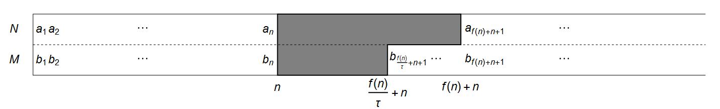 Figure 1
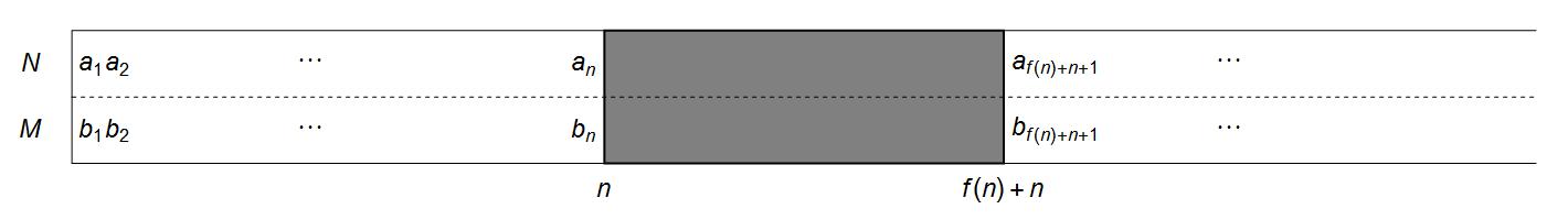 Figure 2
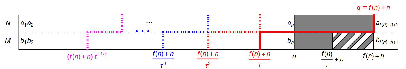 Figure 3
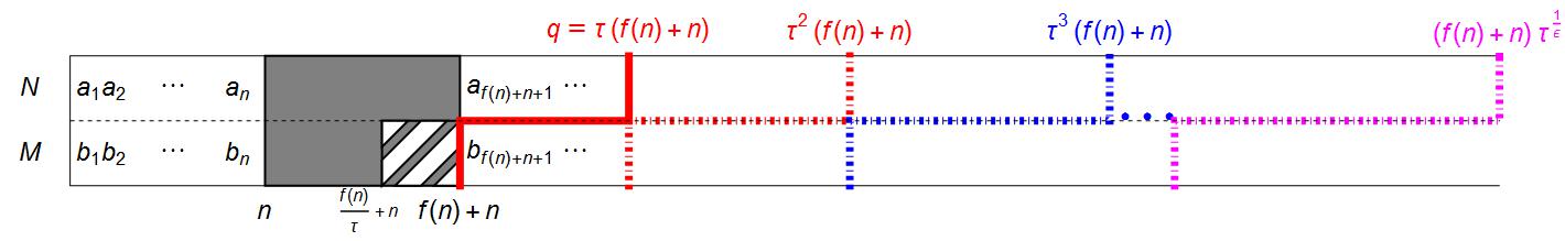 Figure 4
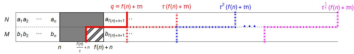 Figure 5
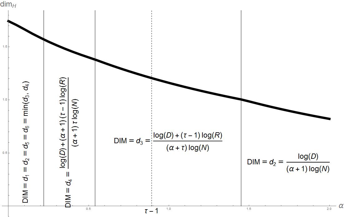 Figure 6
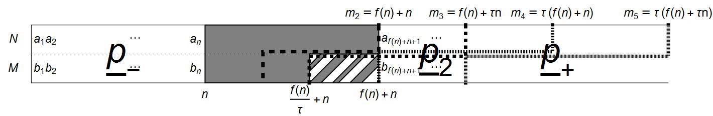 Figure 7
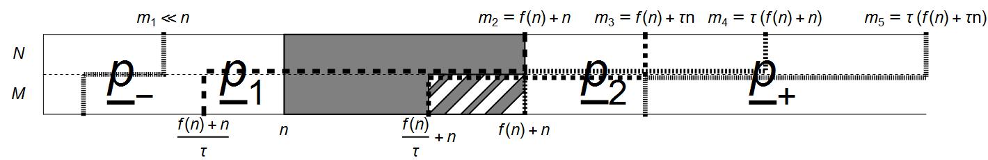 Figure 8
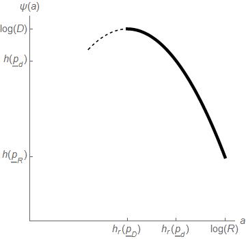 Figure 9