Quantization conditions of eigenvalues for semiclassical Zakharov-Shabat systems on the circle
Setsuro Fujii\'e, Jens Wittsten

TL;DR
This paper derives Bohr-Sommerfeld type quantization conditions for semiclassical eigenvalues of the non-selfadjoint Zakharov-Shabat operator on the circle using an exact WKB method, considering the presence or absence of real turning points.
Contribution
It introduces a novel approach to quantization conditions for non-selfadjoint operators on the circle using exact WKB analysis.
Findings
Quantization conditions depend on the action integral around the circle.
Conditions vary with the presence or absence of real turning points.
Provides a framework for analyzing semiclassical eigenvalues in non-selfadjoint systems.
Abstract
Bohr-Sommerfeld type quantization conditions of semiclassical eigenvalues for the non-selfadjoint Zakharov-Shabat operator on the circle are derived using an exact WKB method. The conditions are given in terms of the action associated with the unit circle or the action associated with turning points following the absence or presence of real turning points.
Click any figure to enlarge with its caption.
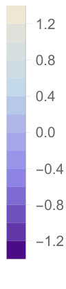 Figure 1
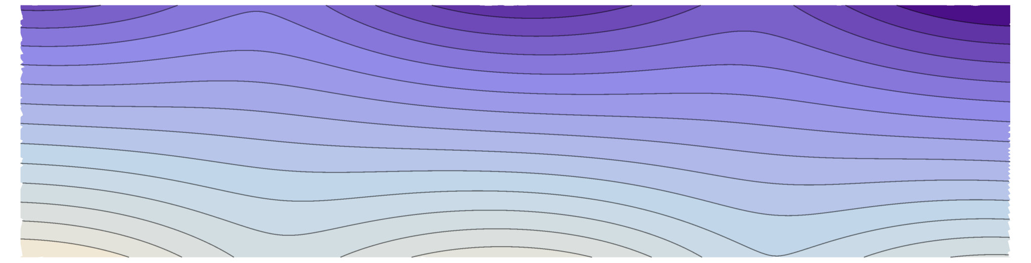 Figure 2
 Figure 3
 Figure 4
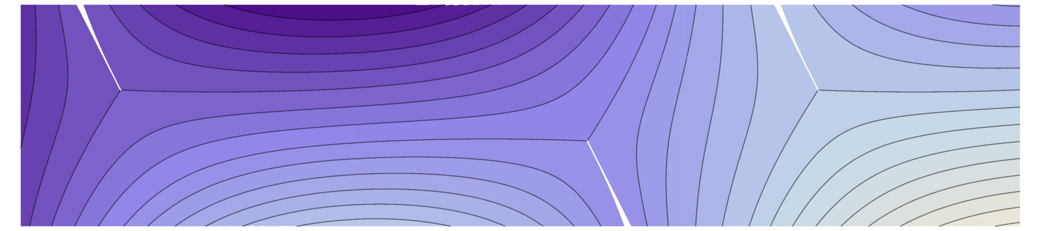 Figure 5
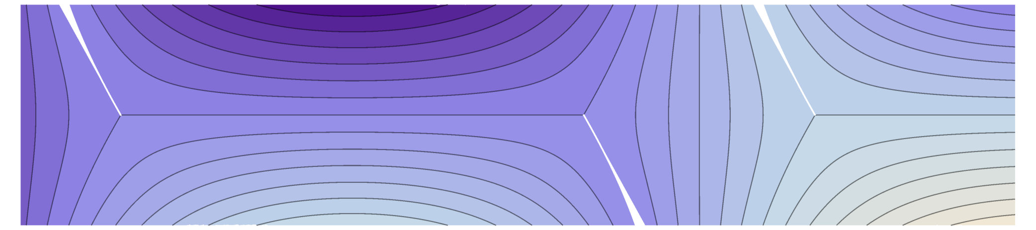 Figure 6
Peer Reviews
No public reviews on file for this paper yet. If you reviewed it on a platform where reviews are public (OpenReview, ICLR, NeurIPS, ICML), you can paste yours below so the community can read it here.
Videos
No videos yet. Explain this paper in a talk, walkthrough, or lecture? Add one.
Jens Wittsten]Centre for Mathematical Sciences, Lund University, Box 118, 221 00, Lund, Sweden
Quantization conditions of eigenvalues for semiclassical
Zakharov-Shabat systems on the circle
Setsuro Fujiié
Department of Mathematical Sciences, Ritsumeikan University, Kusatsu, 525-8577, Japan
and
Jens Wittsten
Department of Mathematical Sciences, Ritsumeikan University, Kusatsu, 525-8577, Japan [ [email protected]
Abstract.
Bohr-Sommerfeld type quantization conditions of semiclassical eigenvalues for the non-selfadjoint Zakharov-Shabat operator on the unit circle are derived using an exact WKB method. The conditions are given in terms of the action associated with the unit circle or the action associated with turning points following the absence or presence of real turning points.
Key words and phrases:
Zakharov-Shabat system, eigenvalues, quantization condition, exact WKB method, transition matrix
2010 Mathematics Subject Classification:
34L40 (primary), 81Q20 (secondary)
1. Introduction
We consider the eigenvalue problem
[TABLE]
for the Zakharov-Shabat operator
[TABLE]
where is a column vector, is a small positive parameter, is a spectral parameter, and is a real valued analytic function on . The eigenvalue problem (1.1) appears in the inverse scattering method for the initial value problem for the focusing nonlinear Schrödinger equation as one half of the Lax pair [16]. It will also be written in the form
[TABLE]
The operator is not selfadjoint. To study the spectrum , let
[TABLE]
be the semiclassical symbol of the operator . We define the closure of the set of eigenvalues of by
[TABLE]
where denotes the determinant of the matrix . Thus, in our case
[TABLE]
where . By Proposition 2.1 below, the spectrum of is discrete and concentrates on as . Hence, to study its asymptotic form one can assume that the spectral parameter belongs to a small neighborhood of .
Before stating our main results, we recall that the roots of , or equivalently,
[TABLE]
are called turning points of the system (1.2). A zero of order of is called a turning point of order . When or , the turning point is said to be simple or double, respectively. When , the simple zeros of are double turning points. Double (or higher order) turning points also occur when and is a local extreme value of . There are no real turning points for non-zero real , and if is strictly positive, then there are no real turning points for with .
To describe the asymptotic distribution of eigenvalues in the semiclassical limit, we fix and study the quantization condition of eigenvalues in a small complex neighborhood of . The form of the quantization condition depends on whether there are real turning points for . We begin with the turning point free case, which is considerably easier. Let denote the disc of radius centered at . We then have the following Bohr-Sommerfeld type quantization condition associated with the action integral along given by
[TABLE]
Theorem 1.1**.**
Let if or if . Then there exists an and a function , analytic with respect to in and uniformly of as , such that is an eigenvalue of if and only if
[TABLE]
In particular, for any small there is an integer such that
[TABLE]
Next we consider , , for which there is at least one real turning point. In view of the symmetry of the eigenvalues with respect to the real axis (Lemma 2.3), it is enough to consider . In this paper, we only consider those for which the turning points are all simple. This implies that the turning points for with close enough to stay simple and depend analytically on (in what follows, is reserved for the complex number defined via ). For each such , there are an even number of turning points which, for real , are real and ordered by . Assuming without loss of generality that , we have that is positive and for , , with the convention . We define two kinds of action integrals and for , which are real for real close to , by
[TABLE]
Theorem 1.2**.**
Suppose , , and that the turning points are all simple. Then there exists an and a function , analytic with respect to in and uniformly of as , such that is an eigenvalue of if and only if
[TABLE]
In particular, for any small there are integers and such that
[TABLE]
This work was first inspired by the paper by Galtsev and Shafarevich [8] who treated the Schrödinger operator with complex potential on . They showed that the spectrum of this non-selfadjoint operator concentrates on a rotated ‘Y’ shape in the semiclassical limit while the set is the half band . This fact has also been used by Dyatlov and Zworski [3] to provide a negative example of stochastic stability of resonances in the context of Anosov flows. The numerical range of our operator , on the contrary, is included in the real and imaginary axes and the spectrum concentrates on the whole numerical range. Thus, does not share the behavior of whose spectrum concentrates on a thin subset of . On the other hand, the fact that is just lines actually specifies the Stokes geometry near the real axis, which allows us to treat general potentials.
To obtain the quantization conditions, we use the exact WKB method along the lines of [6], first introduced by Ecalle [4] and used by Gérard and Grigis [9] to study the Schrödinger operator. An exact WKB solution is a convergent resummation of the WKB asymptotic expansion in a turning-point-free complex region, and the connections of such solutions in different regions via the Wronskian formula (see §2.2) enable us to get the global asymptotic behavior of solutions which leads to the quantization condition of eigenvalues. The asymptotic property of the exact WKB solution is valid only away from turning points, and this prevents us from computing the Wronskian between two exact WKB solutions whose common region of validity is pinched by two turning points close to each other (of distance ). That is why we exclude energies near for which has double or higher order turning points.
The main difference compared with the Schrödinger case is that for our Zakharov-Shabat operator there are two types of turning points, ones of which are the zeros of and the others of which are the zeros of . The phase function of the WKB solutions is a primitive function of the square root of their product while the amplitude is a function of the fourth root of their quotient (see (2.4)). This means that the same Stokes geometry, determined by the phase function, may produce different so-called transition matrices (describing the connections between WKB solutions in different domains) according to the type of intermediate turning points. However, it turns out that the trace of the transition matrix is essentially unaffected (see Proposition 4.4) which explains why there is no mention in Theorem 1.2 of the type of turning points involved. This is not the case in the recent work by Hirota [11] about the eigenvalue problem for a semiclassical Zakharov-Shabat operator (corresponding to the defocusing nonlinear Schrödinger equation) on the real line. In [11], two cases are studied: a simple well potential (two turning points of the same type), and a monotone potential (two turning points of opposite type), resulting in different quantization conditions for the corresponding Zakharov-Shabat system. In our study, there are necessarily an even number of turning points by periodicity, which corresponds (in spirit) to the case of a simple well potential in [11].
Here we also mention the study of Grébert and Kappeler [10] of the periodic eigenvalues of a Zakharov-Shabat operator in the high-energy regime. The problem in the high-energy limit is equivalent to that in the semiclassical limit with a fixed positive energy and with a potential of order . This small potential can be regarded as a small perturbation which does not affect the principal asymptotics of the eigenvalue distribution, and a slight modification of Theorem 1.1 would give (1.5) with , the action for .
The study of non-selfadjoint Zakharov-Shabat systems on the real line has a long history in connection with inverse scattering theory. For the study in the semiclassical limit, we refer to the book by Kamvissis, McLaughlin and Miller [12]. Real energies belong to the continuous spectrum and the reflection coefficient is relevant. Energies near the imaginary axis consist of eigenvalues when decays at infinity, and has a band structure when is periodic (see for example Korotyaev and Kargaev [14]).
The paper is organized as follows. The exact WKB method is reviewed in Section 2, while Section 3 contains the proof of Theorem 1.1. The proof of Theorem 1.2 is the content of Section 4. A crucial detail is the computation of structure formulas for the transition matrices, which for Theorem 1.2 is a much more involved and delicate affair. These computations can be found in Section 5.
2. Preliminaries
We identify with the fundamental domain , and with a -periodic function on . In this context we regard the symbol in (1.3) as a function on which is periodic in , and as an operator acting on vector-valued periodic functions on belonging to . As mentioned in the introduction, for small it suffices to study the case when belongs to a small neighborhood of the set of eigenvalues of the symbol .
Proposition 2.1**.**
For in the resolvent set, is a compact operator and has discrete spectrum. Moreover, if is an open connected set such that , then is a holomorphic function of provided that is sufficiently small.
Proof.
By [13, Theorem 6.29] the first statement follows if we show that is a compact operator for some in the resolvent set. For such we have by the calculus, where denotes the semiclassical pseudodifferential operators of order . In view of the theorem of Rellich and Kondrachov (see e.g., [1, Section 6.3]) this implies that is compact on .
To prove the second statement we shall adapt the arguments of Dencker [2] to our situation. Note that the symbol is also the principal symbol of , and that when we regard as a function on the interior of consists of those for which for some . Similarly, we introduce the eigenvalues at infinity,
[TABLE]
which is easily seen to be closed in by taking a suitable diagonal sequence. We now claim that in our case. Indeed, by definition. Conversely, let , then as for some and . We cannot have since this would imply that if is sufficiently large. Since and are also bounded, we find by restricting to a subsequence and passing to the limit as that
[TABLE]
where and belongs to the set of values of . But then which proves the claim.
Next, using the weight we introduce the symbol classes , , of matrix valued such that
[TABLE]
where denotes the norm of the matrix . Then . Using the Frobenius norm which satisfies , one easily checks that when . If we thus find by [2, Proposition 2.20] that is invertible111Actually, [2, Proposition 2.20] concerns systems on but the claim follows by inspection of the proof together with the fact that symbols in yield bounded operators on by (an extension of) [17, Theorem 5.5]. for sufficiently small , so we can define
[TABLE]
and by the calculus, the symbol of is in , i.e., the symbol and all its derivatives are bounded. We take which is possible by assumption. Now,
[TABLE]
so if and only if for some . Note that since . If , then is an open connected set such that . By [2, Proposition 2.19] it follows that is holomorphic in for sufficiently small. Since the resolvents of and are related by
[TABLE]
the result follows. ∎
2.1. Exact WKB solutions
Here we recall the construction of a solution of (1.2) in a complex domain as a convergent series. Since is real analytic and periodic, it follows that there is a such that extends to a holomorphic function in the strip
[TABLE]
The exact WKB solutions of systems of type (1.2) are known to be of the form
[TABLE]
see [6]. The function is the complex change of coordinates
[TABLE]
where is a base point in . Here, is defined on the Riemann surface of over , and is the matrix valued function
[TABLE]
defined on the Riemann surface of over . These Riemann surfaces are defined by introducing branch cuts emanating from the zeros of , i.e., of (the turning points of the system (1.2)), see Section 4.
The amplitude vectors in (2.2) are defined as the (formal) series
[TABLE]
where , while for are the unique solutions to the scalar transport equations
[TABLE]
[TABLE]
with prescribed initial conditions for some choice of base point where is not a turning point. Here is defined through the chain rule, e.g.,
[TABLE]
Note that these equations are the same as those obtained by an exact WKB construction for scalar Schrödinger equations [9, 15]. When we want to signify the dependence on the base point we write
[TABLE]
for the amplitude vectors.
Let be a simply connected open subset of , free from turning points. Then is conformal from onto . For fixed , the formal series (2.5) converges uniformly in a neighborhood of the amplitude base point , and and are analytic functions in , see [6, Lemma 3.2]. It follows that the functions given by (2.2) are exact solutions of (1.2). They shall henceforth be written as
[TABLE]
to indicate the particular choice of amplitude base point , and phase base point as it appears in (2.3). Note that these solutions are defined for example everywhere on , although some of the expressions involved are only defined on Riemann surfaces of or .
For fixed , let be the set of points for which there is a path from to along which is strictly increasing. In other words, if there is a path which intersects the Stokes lines (i.e., the level curves of ) transversally in the appropriate direction. The calculation of the quantization condition will rely on the following asymptotic properties.
Remark 2.2*.*
For any
[TABLE]
[TABLE]
uniformly on compact subsets of as , see [6, Proposition 3.3]. In particular,
[TABLE]
as .
2.2. The Wronskian formula
For vector valued solutions and of (1.2), we introduce the Wronskian
[TABLE]
Since the trace of the matrix is zero, is actually independent of . For a phase base point and different amplitude base points , elementary computations show that
[TABLE]
where are given by (2.2) via (2.9), and we used the fact that . Since the Wronskian is independent of , we can choose , which in view of the initial conditions of the transport equations (2.6)–(2.7) means that the expression above reduces to
[TABLE]
We may of course also choose , thus obtaining
[TABLE]
In particular, we see that if there is a path from to along which the function is strictly increasing, then as by Remark 2.2. This shows that such a pair of solutions is linearly independent if is sufficiently small.
We shall also need the following formula, obtained by elementary computations, for pairs of solutions of the same type:
[TABLE]
In particular, if we can choose so that it follows that as for some .
2.3. Conjugation
Let denote the scalar complex conjugate of . For a matrix , let denote the matrix with complex conjugated entries, so that is the conjugate transpose (adjoint). For clarity we shall in this subsection write for a solution to (1.2). By using (2.2) and (2.6)–(2.7) it is straightforward to check (see the proof of Lemma 5.4 below) that the WKB solutions enjoy the symmetry property
[TABLE]
This implies that it suffices to study the spectral problem for spectral parameter with nonnegative imaginary part.
Lemma 2.3**.**
The set of eigenvalues of is symmetric with respect to the real axis.
Proof.
Let be an eigenvalue with -periodic eigenvector . Introduce a pair of linearly independent WKB solutions . Since the solution space of (1.2) is -dimensional we have , . Set
[TABLE]
Then is -periodic. Moreover, (2.13) implies that for . Hence, , which completes the proof. ∎
2.4. Periodic solutions
As a final preparation, we record a tractable condition for the existence of a nontrivial periodic solution of (1.2), i.e., an eigenvector of corresponding to .
Proposition 2.4**.**
Let and be a pair of linearly independent solutions of (1.2), and set and . Let be the transition matrix given by
[TABLE]
where is the system with columns and . Then , and the existence of a nontrivial periodic solution of (1.2) is equivalent to the condition
[TABLE]
Proof.
Taking the determinant of both sides of (2.14) we get
[TABLE]
and since the Wronskian is independent of it follows that . Hence, (2.15) is equivalent to , i.e., , which holds if and only if for some vector . If then a simple computation shows that is nontrivial and -periodic. Conversely, if is a nontrivial -periodic solution then can be expressed as a linear combination , and the same computation as before shows that satisfies . ∎
3. Eigenvalues in the absence of real turning points
Here we prove Theorem 1.1 by computing the trace of the transition matrix introduced above, then applying (2.15) and analyzing the result. We fix satisfying the hypotheses of Theorem 1.1, then for all and there are no turning points on the real axis. Choose a determination of
[TABLE]
by picking the branch of the square root satisfying at . Clearly, is independent of , so the real axis is a Stokes line. Since Stokes lines cannot intersect (see e.g. [5]) we find by restricting to a sufficiently small tubular neighborhood of (which in particular should contain no turning points) that the Stokes lines are essentially parallel to the real axis there. Recall that away from turning points, the configuration of Stokes lines depends continuously on the parameter . Hence, we can find such that if then there is a turning-point-free neighborhood of the real axis in which the imaginary axis is still transversal to the tangent vectors of any Stokes line. From now on, we fix . We also choose so small that has positive real part at . This gives a determination of for this choice of which is consistent with the determination of above.
Recall that the number of Stokes lines starting from a turning point of order is . If , the Stokes lines starting from have argument
[TABLE]
see the study by Gérard and Grigis [9, p. 152].
Example 3.1**.**
Let . For , the turning points are simple, and can be found by solving for , where . Upon taking logarithms we get
[TABLE]
Here, and lie in the upper half plane, and and in the lower, and it is easy to check that
[TABLE]
Hence, Stokes lines starting from turning points in the upper half plane have arguments mod . Stokes lines starting from turning points in the lower half plane have arguments mod . Figure 1 shows the configuration of Stokes lines for and .
Note that if we let along the real line in Example 3.1, then the turning points collapse onto the real line to form double turning points, so that case is excluded from Theorem 1.1. For example, and collapse to . The Stokes lines starting from the resulting turning points have argument 0 mod .
We now return to the general situation treated in Theorem 1.1. For near 0 we get by Taylor’s formula
[TABLE]
where is analytic and . Moreover, is approximately real by assumption. Hence, for near 0 we have , showing that is a strictly decreasing function of for near 0. This remains true in a small tubular neighborhood of the real axis, since there, any line parallel to the imaginary axis is transversal to the Stokes lines. The reader is asked to compare with Figure 1.
Let be an amplitude base point in the upper half plane near the real axis with , and let be the complex conjugate. We will choose phase base points on the real line. With the previous discussion in mind, and because we want our WKB solutions to have asymptotic formulas valid in intersecting domains, we introduce the four WKB solutions
[TABLE]
defined in accordance with (2.9). Inspecting the definition (see (2.6)–(2.7)) we find that , so Proposition 2.4 is applicable.
Proposition 3.2**.**
Let be the transition matrix defined by and let denote the action integral . Then
[TABLE]
where . Moreover, where depends holomorphically on , and while for some as .
Proof.
Introduce the auxiliary solutions
[TABLE]
which differ from and only in the choice of phase base point. If is the transition matrix defined by , then a simple computation gives
[TABLE]
with given above.
We next determine , noting that since by Proposition 2.4. Taking Wronskians we get
[TABLE]
We first compute . By the properties of , we can find a curve from (in the upper half plane) to (in the lower half plane) along which is strictly increasing. Evaluating the Wronskian at (see (2.10)) we obtain
[TABLE]
which is by Remark 2.2. Since we can also find curves from to and from to along which is strictly increasing, the same arguments show that
[TABLE]
and both are equal to . Since depends analytically on we find that , where is analytic in and as .
For and , we use the Wronskian formula (2.12) for solutions of the same type. For , we evaluate (2.12) at the point above 0 for some small . Then , so is exponentially decreasing as . For , we evaluate (2.12) at the point below 0. Then , so is exponentially decreasing as . Hence,
[TABLE]
for some , which completes the proof. ∎
End of Proof of Theorem 1.1.
By Proposition 2.4 it follows that is an eigenvalue of if and only if , i.e.,
[TABLE]
which is easily seen to yield (1.4). Multiplying with and completing the square, an elementary computation using gives
[TABLE]
where . Hence, . Taking logarithms we conclude that there is an integer such that
[TABLE]
This gives the desired quantization condition (1.5). ∎
4. Eigenvalues in the presence of real turning points
We now turn to the proof of Theorem 1.2, and we let with be fixed. By assumption, all turning points for are simple. As in Section 3 we begin by describing the configuration of Stokes lines for before turning to general parameter values close to .
4.1. Turning points
As described in the introduction there are turning points
[TABLE]
Since is a local maximum, must be a simple zero of . Thus, and by (3.1) we have
[TABLE]
so the Stokes lines starting at have arguments mod . Basic calculus shows that , so the Stokes lines starting at have arguments [math] mod . A moments reflection shows that this pattern repeats itself, with the Stokes lines starting at odd numbered turning points having arguments mod , and the Stokes lines starting at even numbered turning points having arguments [math] mod ; by periodicity, this includes the last turning point on . In particular, we see that there are bounded Stokes lines lying on starting from even numbered turning points (on the left) and ending at odd numbered turning points (on the right). However, note that this is not a stable configuration and will not persist when is perturbed off the imaginary axis.
We take
[TABLE]
where the choice of turning point will depend on the domain of interest, see (4.2)–(4.3) below. We define the Riemann surfaces of and over by introducing branch cuts from odd numbered turning points along the Stokes lines with argument , and from even numbered turning points along the Stokes lines with argument . We choose branches so that
[TABLE]
Since , this also gives a determination of and therefore of , namely, at the origin. By applying (3.2) with we see that is a strictly decreasing function of for near 0. This determines the behavior of in any simply connected open set that intersects the imaginary axis, does not contain any turning points, and does not pass through a branch cut. In particular, there is also for each a region between and where is a strictly decreasing function of .
When is perturbed through rotation around the origin, the turning points are rotated around points on the real axis, e.g., and are rotated around the mid point , see [7]. Each bounded Stokes line lying on will then split into two unbounded Stokes lines, but with the topology of the Stokes configuration otherwise unchanged. If the perturbation is allowed to continue, then at a rotation angle of around new bounded Stokes lines will appear between simple turning points, and these lines will coincide with the integration paths of the action integrals defined by (1.6). The first change is not significant for the proof of Theorem 1.2, while the second change completely alters the behavior of and is not permitted. From now on we therefore fix such that the integration paths of are not bounded Stokes lines when , and we make sure that
[TABLE]
We also take so small that if is purely imaginary, then the turning points are simple and the Stokes configuration is the same as for ; in particular this means that does not contain [math] and . Moreover, the arguments of Stokes lines at the turning points will be almost unchanged, so we place branch cuts as described for , modified in the obvious manner. We also use the inherited determination of and , namely the one which has positive real part at the origin. Figure 2 illustrates the configuration of Stokes lines near three consecutive turning points, including the location of branch cuts.
4.2. The transition matrix
Under the assumptions of Theorem 1.2, the transition matrix , as defined in Proposition 2.4, will consist of a product of intermediate transition matrices. These matrices will be of (at most) four types, which we now describe.
Let . We fix amplitude base points in the upper half plane independent of as in Figure 3 in such a way that and so that is always in the same region bounded by Stokes lines when varies in . We then set . Introduce the WKB solutions
[TABLE]
defined for in accordance with (2.9), where . The transition from the pair to the pair is one of the following four kinds:
- .
Both and are zeros of .
- .
is a zero of and is a zero of .
- .
is a zero of and is a zero of .
- .
Both and are zeros of .
That there are no other kinds follows from the fact that since , the nature of the zeros and also determines the nature of , e.g., if both and are zeros of then so is . Introduce also the auxiliary solutions
[TABLE]
Let (resp. ) be the transition matrix between and (resp. between and ):
[TABLE]
For each for it is clear that is of the same transition type as . The transition matrix as defined in Proposition 2.4 is given by
[TABLE]
Example 4.1**.**
In the case where and with , there are four turning points (i.e. ), and . The matrix is of type and is of type . In the case where and with , there are two turning points (i.e. ), and . The matrix is of type .
Recall the definition of the action integrals in (1.6). By straightforward computation we immediately obtain the following relationship between and .
Lemma 4.2**.**
[TABLE]
We now describe the different types of transition matrices.
Theorem 4.3**.**
If is of type , then
[TABLE]
where the matrix depends analytically on in for some positive and is uniformly of there as , and
[TABLE]
We postpone the proof of Theorem 4.3 to Section 5, where it will be an immediate consequence of Theorem 5.1 and Theorems 5.6–5.8 together with Lemma 4.2.
4.3. Computing the trace
By (4.5), is a product of matrices of transitions – , the precise nature of which depends on the potential . However, in a sense made precise below, the trace of does not. Note that there are some restrictions on the possible factors in a product of intermediate transition matrices such as (4.5): if we for the moment write to indicate that is a transition matrix of type , then (4.5) cannot contain any of the factors
[TABLE]
and by periodicity it must contain an equal number of matrices of transitions and .
Proposition 4.4**.**
For let be given by (4.5). Then
[TABLE]
where depends analytically on in and is uniformly of there as .
Proof.
For we let with the convention that , and set
[TABLE]
In view of Theorem 4.3, the result follows if we show that
[TABLE]
It is straightforward to check that for each we have
[TABLE]
and that as a result thereof
[TABLE]
Now, (4.6) is clearly true when , since is necessarily of type or then, i.e., or . When all the are of type , it is easy to see that (4.6) holds with on the right by using induction with respect to and applying (4.7) with , and . If all the are of type one obtains (4.6) with on the right in the same way.
It remains to prove (4.6) when contains at least one pair of matrices of type and . Write
[TABLE]
and say that is of type if . Since the trace is invariant under cyclic permutations, we may without loss of generality assume that is of type . To the left of there must be a block of type matrices of length , followed by a type matrix. If then the first paragraph shows that this block of type matrices is equal to . It is then easy to see that
[TABLE]
Now, to the left of this block there can be a block of type matrices of length , followed by another block of the same kind as of length , and this is repeated a finite number of times until the left-hand side of (4.6) is exhausted. But since both types of blocks have already been treated, (4.6) follows by virtue of (4.7). ∎
End of Proof of Theorem 1.2.
Let be given by (4.5). By Proposition 2.4, is an eigenvalue of if and only if . For , we thus obtain (1.7) by applying Proposition 4.4. In particular, (4.1) gives
[TABLE]
Hence, for some we must have , so
[TABLE]
which yields the quantization condition (1.8) and the proof is complete. ∎
5. Structure results for transition matrices
Here we prove Theorem 4.3 by studying each matrix of transition – separately, starting with transition . In view of Lemma 4.2 it suffices to consider the auxiliary transition matrices .
Theorem 5.1**.**
Let be the transition matrix defined by (4.4). If is of type then
[TABLE]
where depend analytically on in and are there equal to uniformly as , and where is the action integral given by (1.6).
Before providing the full details of the proof, which requires some preparation, we briefly sketch the main idea: Write . Taking Wronskians in (4.4) we get
[TABLE]
Here, and can easily be computed using (2.10) and then estimated using Remark 2.2. However, in contrast to the case studied in Theorem 1.1, we will not be able to use the Wronskian formula (2.12) for solutions of the same type to handle and , for these will no longer exhibit the same rapid decay. Instead, we shall express one of the WKB solutions in each Wronskian in the coordinates of a different sheet of the Riemann surface, thereby changing the type from to . We can then use (2.10) to compute the Wronskian as normal, and estimate the result using Remark 2.2. For the computation of , the presence of branch cuts means that although the WKB solutions already are of different type, similar techniques have to be used to ensure that Remark 2.2 is applicable.
The following observations are stated in sufficient generality to be useful in the sequel, but to anchor the discussion we use the assumptions of Theorem 5.1 as starting point, with primary goal of rewriting as a solution of type in order to allow for the computation of . Let denote the operator acting through rotation around by radians, so that, e.g., . Since is analytic it follows that if then
[TABLE]
i.e., when is rotated radians anticlockwise around then is rotated radians anticlockwise around the origin. (Negative results in clockwise rotation by radians.) We of course have similar behavior for when .
Definition 5.2**.**
Let be a turning point such that (transitions and ). The point over that is obtained when rotating clockwise once around will be denoted by , i.e.,
[TABLE]
More generally, the sheet reached (from the usual sheet) by entering the cut starting at from the left will be referred to as the -sheet. The point over that is obtained when rotating anticlockwise once around will be denoted by , i.e.,
[TABLE]
The sheet reached (from the usual sheet) by entering the cut starting at from the right will be referred to as the -sheet. If instead (transitions and ) then all directions are to be reversed.
When winding this way around a turning point we always assume that the path is appropriately deformed so as not to be obstructed by other branch cuts. Informally, we think of as lying in the sheet “above” the usual sheet, and as lying in the sheet “below” the usual sheet. The next lemma describes the relative direction of the branch cut starting at .
Lemma 5.3**.**
If then the -sheet is reached (from the usual sheet) by rotating anticlockwise once around , i.e., by entering the cut from the left. The -sheet is reached (from the usual sheet) by rotating clockwise once around . If instead then the directions are reversed. Moreover,
[TABLE]
The reason for wanting to reverse the directions in Definition 5.2 when is to make sure that (5.3)–(5.4) are always in force. In fact, these identities can be taken as definitions of the sheets.
Proof.
Assume first that . Fix a point on the line segment from to in the area between the cuts, then . When is rotated radians around , is rotated radians around the origin, so
[TABLE]
If instead , then , which by (5.2) again yields
[TABLE]
Hence, (5.3) is still in force. One proves (5.4) in the same way.
Next, suppose that . To see that the -sheet is reached by entering the cut starting at from the left, take on the line segment from to and note that
[TABLE]
thus , which means that . (For a fixed point , takes distinct values at each of the four points over .) In the same way one proves the statement concerning the -sheet, as well as the reverse statements when . We omit the details. ∎
In order to compute we want to express in the coordinates of a different sheet over , and continue the resulting function through the branch cut into the domain of in the usual sheet (containing the amplitude base point ), so that their domains intersect and (2.10) and Remark 2.2 are applicable. Under the assumptions of Theorem 5.1 (transition ), entering the branch cut starting at from the left leads to the -sheet by Definition 5.2, so this means rewriting in the coordinates of the -sheet. (The same is true for transition ; for transitions and it means rewriting in the coordinates of the -sheet.) Recall that , which by definition means that for near in the usual sheet we have
[TABLE]
where
[TABLE]
The change of variables gives
[TABLE]
Using the shorthand , , we have by (5.3), so the definition of (see (2.4)) gives
[TABLE]
Note that squaring the rightmost matrix gives the identity matrix.
Next, we express in the coordinates of the -sheet. To this end, let , , be a family of solutions to the transport equations (2.6)–(2.7), satisfying the initial conditions at . Set , . Inspecting (2.6)–(2.7) and using , it is easy to check that
[TABLE]
[TABLE]
with at . By uniqueness of solutions it follows that with , which, in view of (2.5), implies that
[TABLE]
In particular, , which together with (5.5)–(5.7) gives
[TABLE]
for near . This proves the first part of the following lemma.
Lemma 5.4**.**
For each transition – , let and be defined in accordance with Definition 5.2. Then
[TABLE]
Proof.
The arguments above show that . Since , the identity follows by using the same arguments except with (5.4) used in place of (5.3). It remains to prove the identities for the turning point . But since (compare with (5.6)) and
[TABLE]
the first identity is a consequence of (5.7) and (5.8), while the second again follows by similar arguments except with (5.4) used in place of (5.3). ∎
It will be convenient to record the following observation.
Lemma 5.5**.**
Let be given by (1.6). Then
[TABLE]
Proof.
It suffices to prove (5.9) for , for then the general result follows by continuity. To evaluate the right-hand side of (5.9) when is real, note that the line segment from to is an interval on the real line. Next, recall that we have chosen a determination of so that it is positive at the origin, or in fact at any point in the same sheet as the origin where . In particular, for real close to . For real close to we write
[TABLE]
with as above (rotation in the opposite direction is incorrect since it means passing through a branch cut). Hence, the right-hand side of (5.9) equals
[TABLE]
where the integrand in the rightmost integral is non-negative by (5.10). The lemma now follows by inspecting the definition of . ∎
Proof of Theorem 5.1.
Recalling (5.1), we first compute . According to the behavior of , there is a curve from to along which is strictly increasing. By evaluating the Wronskian at (see (2.10)) we get
[TABLE]
where by Remark 2.2.
Now consider and note that the phase base points of and differ. We therefore rewrite as
[TABLE]
where the last identity follows by virtue of Lemma 5.5. Since we can find a curve along which is strictly increasing we can evaluate the Wronskian at (see (2.10)) and get
[TABLE]
where by Remark 2.2. Thus, by (5.1) and (5.11) we have
[TABLE]
It is clear that depends analytically on since this is true for the amplitude functions .
We now compute . By Lemma 5.4 we have for near . Take the function on the right and continue it through the branch cut starting at into the domain in the usual sheet containing . We remark that at it takes the value . Similarly, writing as before, we see that , so by evaluating the Wronskian at (see (2.10)) we get
[TABLE]
Since is a strictly increasing function of near , we can find a curve from to , passing through the branch cut at , along which is strictly increasing (compare with Figure 2). Hence, by (5.1), (5.11) and Remark 2.2 we get
[TABLE]
Let us consider next. We fix the domain of and express in the coordinates of the sheet reached when passing through the branch cut at from the left. For transition this is the -sheet according to Definition 5.2. First note that
[TABLE]
compare with (5.12). Applying Lemma 5.4 we get
[TABLE]
We continue the expression on the right through the branch cut at , and note that at , it takes the value . As above we can find a curve from to , passing through the branch cut at , along which is strictly increasing. Hence, by evaluating the Wronskian at (see (2.10)) we obtain
[TABLE]
In view of (5.1), (5.11) and Remark 2.2 we conclude that
[TABLE]
Finally, let us consider . To get an asymptotic estimate we will need to connect the amplitude base points of and by a curve passing through both the branch cut at and the branch cut at . In view of Definition 5.2 this will be possible if we (in the present case of transition ) express in the coordinates obtained by rotating anticlockwise twice around . Let the coordinates thus obtained be denoted . Applying Lemma 5.4 two times we get
[TABLE]
for near . We can find a path from to along which is strictly increasing (compare with Figure 2), so evaluating the Wronskian at we get (see (2.10))
[TABLE]
where as by Remark 2.2. Here,
[TABLE]
where the path of integration is homotopic to a curve starting at and following a curve in the -sheet through the branch cut at , then arriving at via . In other words, it is homotopic to the path from to in the -sheet. If we rotate back to the usual sheet using (5.2) and then reverse the integration direction, we find that
[TABLE]
which by Lemma 5.5 is equal to the action integral given by (1.6). Recalling (5.1), (5.11) we get
[TABLE]
which completes the proof. ∎
We now turn to the matrices of transition , and .
Theorem 5.6**.**
Let be the transition matrix defined by (4.4). If is of type then
[TABLE]
where depend analytically on in and are there equal to uniformly as , and where is the action integral given by (1.6).
Proof.
Write , then is given by (5.1). The proof continues in almost identical fashion to the proof of Theorem 5.1. The only difference is that when rewriting and in order to compute the Wronskians and , respectively, we do so using the coordinates of the -sheet instead of the -sheet, see the discussion preceding (5.5). In view of Lemma 5.4, this results in the loss of a factor in the formulas for and . To compute we apply Lemma 5.4 twice, and since , this leads to the same calculations as in the proof of Theorem 5.1. ∎
Theorem 5.7**.**
Let be the transition matrix defined by (4.4). If is of type then
[TABLE]
where depend analytically on in and are there equal to uniformly as , and where is the action integral given by (1.6).
Proof.
Write , then is given by (5.1). The computation of is the same as for transitions and . Since the nature of is the same as in transition , the computation of (rewriting by rotating around ) is the same as for transition . Since the nature of is the same as in transition , the computation of (rewriting by rotating around ) is the same as for transition . For , we simply compute directly from (2.10) by evaluating the Wronskian at (the amplitude base point of ) and obtain
[TABLE]
In fact, for transition there is, in view of Definition 5.2, a path from to along which is strictly increasing: starting at in the usual sheet, goes through the branch cut at from the right (thereby entering the -sheet), then goes through the branch cut at from the right, reentering the usual sheet and then ending at . In view of the discussion following (5.13), this implies that , which gives
[TABLE]
The proof is complete. ∎
Theorem 5.8**.**
Let be the transition matrix defined by (4.4). If is of type then
[TABLE]
where depend analytically on in and are there equal to uniformly as , and where is the action integral given by (1.6).
Proof.
Write , then is given by (5.1). The computations of and are the same as for transition (except that for , the path from to goes via the -sheet instead), while the computations of and are reversed: Since the nature of is the same as in transition , the computation of (rewriting by rotating around ) is the same as for transition . Since the nature of is the same as in transition , the computation of (rewriting by rotating around ) is the same as for transition . ∎
Acknowledgements
The research of Setsuro Fujiié was supported by the JSPS Kakenhi Grant No. JP15K04971. The research of Jens Wittsten was supported by the Knut och Alice Wallenbergs Stiftelse Grant No. 2013.0347.
The reference list from the paper itself. Each links out to its DOI / PubMed record.
- 1[1] Robert A. Adams and John J. F. Fournier, Sobolev spaces , Pure and Applied Mathematics, vol. 140, Elsevier/Academic Press, 2003.
- 2[2] Nils Dencker, The pseudospectrum of systems of semiclassical operators , Analysis & PDE 1 (2008), 323–373.
- 3[3] Semyon Dyatlov and Maciej Zworski, Stochastic stability of Pollicott–Ruelle resonances , Nonlinearity 28 (2015), no. 10, 3511.
- 4[4] Jean Ecalle, Cinq applications des fonctions résurgentes , Prépublications mathématiques d’Orsay, Département de mathématique, 1984.
- 5[5] Marat A. Evgrafov and Mikhail V. Fedoryuk, Asymptotic behaviour as λ → ∞ → 𝜆 \lambda\to\infty of the solution of the equation w ′′ ( z ) − p ( z , λ ) w ( z ) = 0 superscript 𝑤 ′′ 𝑧 𝑝 𝑧 𝜆 𝑤 𝑧 0 w^{\prime\prime}(z)-p(z,\lambda)w(z)=0 in the complex z 𝑧 z -plane , Russian Mathematical Surveys 21 (1966), 1–48.
- 6[6] Setsuro Fujiié, Caroline Lasser, and Laurence Nédélec, Semiclassical resonances for a two-level Schrödinger operator with a conical intersection , Asymptotic Analysis 65 (2009), no. 1-2, 17–58.
- 7[7] Setsuro Fujiié and Thierry Ramond, Matrice de scattering et résonances associées à une orbite hétérocline , Ann. Inst. H. Poincaré Phys. Théor. 69 (1998), no. 1, 31–82.
- 8[8] Sergei V. Galtsev and Andreĭ I. Shafarevich, Quantized Riemann surfaces and semiclassical spectral series for a non-self-adjoint Schrödinger operator with periodic coefficients , Theoretical and Mathematical Physics 148 (2006), no. 2, 1049–1066.