Structure Preserving Model Reduction of Parametric Hamiltonian Systems
Babak Maboudi Afkham, Jan S. Hesthaven

TL;DR
This paper introduces a structure-preserving greedy model reduction method for parametric Hamiltonian systems that ensures stability and efficiency in long-term simulations by maintaining symplectic structure.
Contribution
It presents a novel greedy basis selection algorithm that preserves symplectic structure and demonstrates exponential convergence for parametric Hamiltonian systems.
Findings
Ensures stability of reduced models over long-time integration.
Achieves exponential convergence of the greedy algorithm.
Preserves symplectic structure when combined with empirical interpolation.
Abstract
While reduced-order models (ROMs) have been popular for efficiently solving large systems of differential equations, the stability of reduced models over long-time integration is of present challenges. We present a greedy approach for ROM generation of parametric Hamiltonian systems that captures the symplectic structure of Hamiltonian systems to ensure stability of the reduced model. Through the greedy selection of basis vectors, two new vectors are added at each iteration to the linear vector space to increase the accuracy of the reduced basis. We use the error in the Hamiltonian due to model reduction as an error indicator to search the parameter space and identify the next best basis vectors. Under natural assumptions on the set of all solutions of the Hamiltonian system under variation of the parameters, we show that the greedy algorithm converges with exponential rate. Moreover,…
Click any figure to enlarge with its caption.
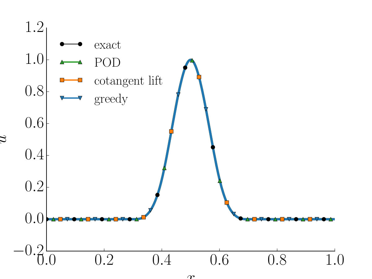 Figure 1
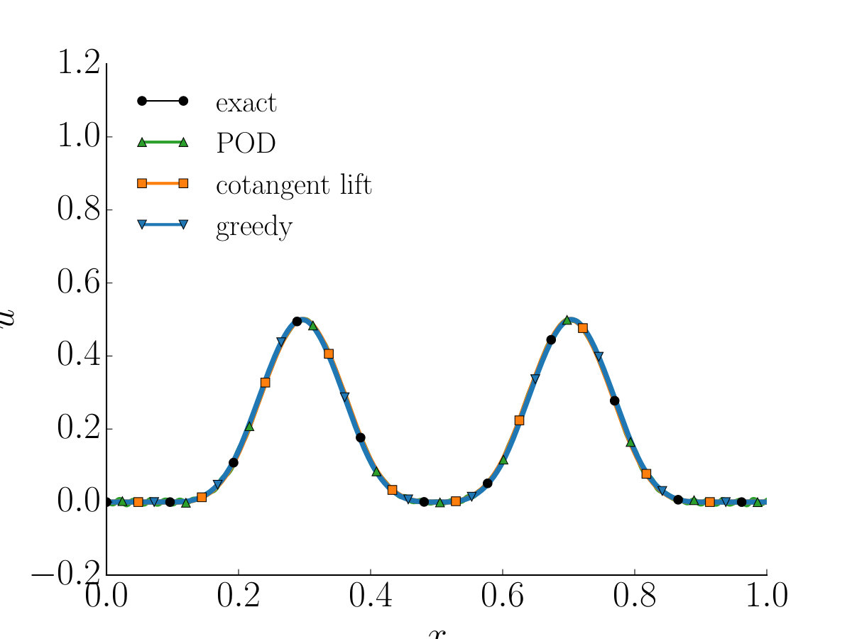 Figure 2
Peer Reviews
No public reviews on file for this paper yet. If you reviewed it on a platform where reviews are public (OpenReview, ICLR, NeurIPS, ICML), you can paste yours below so the community can read it here.
Videos
No videos yet. Explain this paper in a talk, walkthrough, or lecture? Add one.
\headers
Symplectic Model Reduction of Hamiltonian SystemsB. Maboudi Afkham, and J. S. Hesthaven
\externaldocumentex_supplement
Structure Preserving Model Reduction of Parametric Hamiltonian Systems
Babak Maboudi Afkham Department of Mathematics, Chair of Computational Mathematics and Simulation Science (MCSS), École Polytechnique Fédérale de Lausanne, Switzerland () [email protected]
Jan S. Hesthaven Department of Mathematics, Chair of Computational Mathematics and Simulation Schience (MCSS), École Polytechnique Fédérale de Lausanne, Switzerland () [email protected]
Abstract
While reduced-order models (ROMs) have been popular for efficiently solving large systems of differential equations, the stability of reduced models over long-time integration is of present challenges. We present a greedy approach for ROM generation of parametric Hamiltonian systems that captures the symplectic structure of Hamiltonian systems to ensure stability of the reduced model. Through the greedy selection of basis vectors, two new vectors are added at each iteration to the linear vector space to increase the accuracy of the reduced basis. We use the error in the Hamiltonian due to model reduction as an error indicator to search the parameter space and identify the next best basis vectors. Under natural assumptions on the set of all solutions of the Hamiltonian system under variation of the parameters, we show that the greedy algorithm converges with exponential rate. Moreover, we demonstrate that combining the greedy basis with the discrete empirical interpolation method also preserves the symplectic structure. This enables the reduction of the computational cost for nonlinear Hamiltonian systems. The efficiency, accuracy, and stability of this model reduction technique is illustrated through simulations of the parametric wave equation and the parametric Schrödinger equation.
keywords:
Symplectic model reduction, Hamiltonian system, Greedy basis generation, Symplectic Discrete Empirical Interpolation (SDEIM)
{AMS}
1 Introduction
Parameterized partial differential equations often arise as a model in many problems in engineering and the applied sciences. While the need for more accuracy has led to the development of exceedingly complex models, the limitations in computational cost and storage often make direct approaches impractical. Hence, we must seek alternative methods that allow us to approximate the desired output under variation of the input parameters while keeping the computational costs to a minimum.
Reduced basis methods have emerged as a powerful approach for the reduction of the intrinsic complexity of such models [21, 22, 23, 33]. These methods contain two stages: the offline stage and the online stage. In the offline stage, one explores the parameter space to construct a low-dimensional basis that accurately represents the parametrized solution to the partial differential equation. In this stage, the evaluation of the solution of the original model for multiple parameter values is required. The online stage comprises a Galerkin projection onto the span of the reduced basis, which allows exploration of the parameter space at a significantly reduced complexity [2, 20].
Convectional reduced basis techniques, such as proper orthogonal decomposition (POD) [26, 3, 38], require the exploration of the entire parameter space. This leads to a very expensive and often impractical offline stage when dealing with multi-dimensional parameter domains. On the other hand, sampling techniques, usually of a greedy nature, search through the parameter space selectively, guided by an error estimate to certify the accuracy of the basis. This approach, accompanied with an efficient sampling procedure, balances the cost of computation with the overall accuracy of the reduced-basis [15, 39, 20].
Besides computational complexity, another aspect of reduced order modeling is the preservation of structure and, in particular, the stability of the original model. In general, reduced order models do not guarantee that such properties are preserved [36].
In the context of Hamiltonian and Lagrangian systems, recent work suggests modifications of POD to preserve some geometric structures. Lall et al. [27] and Carlberg et al. [12] suggests that the reduced-order system should be identified by a Lagrangian function on a low-dimensional configuration space. In this way, the geometric structure of the original system is inherited by the reduced system. Model reduction for port-Hamiltonian systems can be found in the works of Beattie et al. [13], Polyuga et al. [35] and references therein. These works construct a reduced port-Hamiltonian system using Krylov or POD methods that inherit the passivity and stability of the original system. For Hamiltonian systems, Peng et al. [32], using a symplectic transformation, constructs a reduced Hamiltonian, as an approximation to the Hamiltonian of the original system. As a result, the reduced system preserves the symplectic structure. Although these methods preserve the geometric structure, they use a POD-like approach for constructing the reduced basis and are not well suited for problems with a high-dimensional parameter domain.
In this paper, we present a greedy approach for the construction of a reduced system that preserves the geometric structure of Hamiltonian systems. This technique results in a reduced Hamiltonian system that mimics the symplectic properties of the original system and preserves the Hamiltonian structure and its stability over the course of time. On the other hand, since time integration of the original system is only required once per iteration, the proposed method saves substantial computational cost during the offline stage when compared to alternative POD-like approaches. It is well known that structured matrices, e.g. symplectic matrices, generally are not well-conditioned [24]. The greedy update of the symplectic basis presented here, yields a orthosymplectic basis and, therefore, a norm bounded basis. Moreover, we demonstrate that assumptions, natural for the set of all solutions of the original Hamiltonian system under variation of parameters, lead to exponentially fast convergence of the greedy algorithm. For nonlinear Hamiltonian systems, we show how the basis can be combined with the discrete empirical interpolation method (DEIM) [14, 4] to enable a fast evaluation of nonlinear terms while maintaining the symplectic structure.
This paper is organized as follows. Section 2 presents a brief overview of model order reduction, POD and DEIM. In Section 3 we cover the required topics from symplectic geometry and Hamiltonian systems. Section 4 discusses the greedy generation of a symplectic reduced basis as well as other SVD-based symplectic model reduction techniques. Accuracy, stability, and efficiency of the greedy method compared to other SVD-based methods are discussed in Section 5. Finally we offer some conclusive remarks in Section 6.
2 Model Order Reduction
Consider a parameterized, finite dimensional dynamical system described by a set of first order ordinary differential equations
[TABLE]
Here is the state vector, is a vector containing all the parameters of the system belonging to a compact set () and is a general vector valued function of the state variables and parameters.
We define the solution manifold as the set of all solutions to (1) under variation of the parameters in
[TABLE]
Note that the exact solution and solution manifold is often not available; we assume that we have a numerical integrator that can approximate the solution to (1) for any realization of with a given accuracy. By abuse of notation, we refer to and as the exact solution and the exact solution manifold, respectively, rather than the discrete solution and discrete solution manifold.
Model order reduction is based on the assumption that is of low dimension [20, 2] and that the span of appropriately chosen basis vectors covers most of the solution manifold to within a small error. The set is denoted as the reduced basis and its span as the reduced space. Assuming that a -dimensional reduced basis is given, the approximated solution can be represented as
[TABLE]
where is a matrix containing the reduced basis vectors as its columns and contains the coordinates of the approximation in this basis. By substituting (3) into (1) we obtain the overdetermined system
[TABLE]
Here we added the residual to emphasize that (4) is an approximation of (1). Taking the Petrov-Galerkin projection [2] we construct a basis of size that is orthogonal to the residual and requires that is invertible. This yields
[TABLE]
Equation (5) consists of equations and is called the reduced system. Solving the reduced system instead of the original system can reduce the computational costs provided is significantly smaller than . For nonlinear systems, the evaluation of may still have computational complexity that depends on . We return to this question in detail in Section 2.2.
2.1 Proper Orthogonal Decomposition
Let with and be a finite number of samples, referred to as snapshots, from the solution manifold (2). If we assume that a reduced basis is provided, the projection operator from onto the reduced space can be constructed as . The proper orthogonal decomposition (POD) requires the total error of projecting all the snapshots onto the reduced space to be minimized. The POD basis of size is thus the solution to the optimization problem
[TABLE]
Here is the snapshot matrix, containing snapshots in its columns, is the Frobenius norm and is the identity matrix of size . According to Schmidt-Mirsky-Eckart-Young theorem [28], the solution to (6) is equivalent to the truncated singular value decomposition (SVD) of the snapshot matrix given by
[TABLE]
Here and are the singular values, the left singular vectors, and the right singular vectors of , respectively [28] .
2.2 Discrete Empirical Interpolation Method (DEIM)
In this section we discuss the efficiency of evaluating nonlinearities in the context of projection based reduced models. Suppose that the right hand side in (1) is of the form , where reflects the linear part, and is a nonlinear function. Now assume that a -dimensional reduced basis is provided. The reduced system takes the form
[TABLE]
Here, is a matrix which can be computed before time integration of the reduced system. However, the evaluation of has a complexity that depends on , the size of the original system. Suppose that the evaluation of with components has the complexity , for some function . Then the complexity of evaluating is which consists of 2 matrix-vector operations and the evaluation of the nonlinear function, i.e. the evaluation of the nonlinear terms can be as expensive as solving the original system.
To overcome this bottleneck we take an approach similar to that of Section 2.1 [14, 4]. Assume that the manifold is of a low dimension and that can be approximated by a linear subspace of dimension , spanned by the basis , i.e.
[TABLE]
Here contains basis vectors and is the vector of coefficients. Now suppose are indices from and define an matrix
[TABLE]
where is the -th column of the identity matrix . Multiplying with selects components of . If we assume that is non-singular, the coefficient vector can be uniquely determined from
[TABLE]
Finally the approximation of is determined by
[TABLE]
which is referred to as the Discrete Empirical Interpolation (DEIM) approximation [14]. Applying DEIM to the reduced system (5) yields
[TABLE]
Note that the matrix can be computed offline and since is evaluated only at of its components, the evaluation of the nonlinear term in (13) does not depend on .
To obtain the projection basis , the POD can be applied to the ensemble of samples of the nonlinear term with and . There is no additional cost associated with computing the nonlinear snapshots, since they are generated when computing the trajectory snapshot matrix . The interpolating indices can be constructed as follows. Given the projection basis , the first interpolation index is chosen according to the component of with the largest magnitude. The rest of the interpolation indices, correspond to the component of the largest magnitude of the residual vector . It is shown in [14] that if the residual vector is a nonzero vector in each iteration then is non-singular and (12) is well defined.
The numerical solution of (8) may involve the computation of the Jacobian of the nonlinear function with respect to the reduced state variable
[TABLE]
where is the Jacobian matrix of with respect to the variable . The complexity of (14) is , comprising several matrix-vector multiplications and an evaluation of the Jacobian which depends on the size of the original system. Approximating the Jacobian in (14) is usually both problem and discretization dependent. Often the nonlinear function is evaluated component-wise i.e.
[TABLE]
In such cases the interpolating index matrix and the nonlinear function commute, i.e.,
[TABLE]
If we now take the Jacobian of the approximate function we recover
[TABLE]
The matrix can be computed offline and the Jacobian is evaluated only for components. Hence the overall complexity of computing the Jacobian is now independent of . We refer the reader to [4, 14] for more detail.
3 Hamiltonian Systems and Symplectic Geometry
Let \color[rgb]{0,0,0}\mathcal{M} be a manifold and \color[rgb]{0,0,0}\Omega:\mathcal{M}\times\mathcal{M}\to\mathbb{R} be a closed, nondegenerate and skew-symmetric 2-form on \color[rgb]{0,0,0}\mathcal{M}. The pair \color[rgb]{0,0,0}(\mathcal{M},\Omega) is called a symplectic manifold [29].
Let be a symplectic manifold and suppose that is a smooth scalar function. The differential of , denoted by , defines a 1-form on . The nondegeneracy of implies that there is a unique vector field , *Hamiltonian vector field *[16, 29], on such that
[TABLE]
where is the interior product of with , i.e., that requiring
[TABLE]
for any vector field on . Note that when \color[rgb]{0,0,0}\mathcal{M} belongs to a Euclidean space then . The equations of evolution are then defined by
[TABLE]
and known as Hamilton’s equation [29]. A fundamental feature of Hamiltonian systems is the conservation of the Hamiltonian along integral curves on \color[rgb]{0,0,0}\mathcal{M}. To emphasize the importance of this property we recall [29]
Theorem 3.1**.**
*Suppose that is a Hamiltonian vector field with the flow on a symplectic manifold . Then . *
Proof 3.2**.**
* is constant along integral curves since*
[TABLE]
*by using the chain rule and bilinearity of in the argument. *
For the case where the symplectic manifold is also a linear vector space, the pair ({\color[rgb]{0,0,0}\mathcal{M}},\Omega) is also referred to as a symplectic vector space. We need the following theorems regarding symplectic vector spaces and refer the reader to [17, 29, 17, 11] for detailed proofs.
Theorem 3.3**.**
[29*]** If is a symplectic vector space then is a constant form, that is is independent of . *
Theorem 3.4**.**
[29*]** If is a finite-dimensional symplectic manifold then is even dimensional. *
Theorem 3.5**.**
[17]** (The Symplectic Gram-Schmidt) If is a -dimensional symplectic vector space, then there is a basis of such that
[TABLE]
where is the Kronecker’s delta function. Moreover if we can choose basis vectors such that
[TABLE]
with being the symplectic matrix, defined as
[TABLE]
*Here and is the identity matrix and the zero square matrix of size , respectively. *
Theorem 3.6**.**
[29]** The classical inner product can be written in terms of the 2-form as
[TABLE]
Definition 3.7**.**
[17]** Suppose is a finite dimensional symplectic vector space and is a subspace. Then the symplectic complement of inside is defined as
[TABLE]
Note that is not empty in general.
Definition 3.8**.**
[17*]** Suppose is a finite dimensional symplectic vector space. A subspace is called a Lagrangian subspace inside if . *
Theorem 3.9**.**
[1*]** Suppose is a finite dimensional symplectic vector space. If is a Lagrangian subspace then . Here denotes the dimension of the subspace. *
Definition 3.10**.**
*A basis of is called orthosymplectic if it is both a symplectic basis and an orthogonal basis with respect to the classical scalar product. *
Theorem 3.11**.**
[16*]** Suppose is a dimensional symplectic vector space and is a Lagrangian subspace. Then there is an orthosymplectic basis for . *
Proof 3.12**.**
Starting from a Lagrangain subspace in an orthosymplectic basis can be easily constructed. By Theorem 3.9 is dimensional. Suppose that is a basis for , using the classical Gram-Schmidt orthogonalization process we can construct an orthonormal basis . Define a new set of vectors , , , . We have
[TABLE]
*where we used the fact that in the first identity and the second identity is due to the fact that the basis forms a Lagrangian subspace. This shows that the set forms an orthonormal basis. Also, it can be easily verified that this is a symplectic basis. Thus is an orthosymplectic basis. *
Theorem 3.13**.**
[29]** On a finite-dimensional symplectic vector space the relationship (18) becomes
[TABLE]
or, by introducing the canonical coordinates ,
[TABLE]
Let us now introduce symplectic transformations, i.e., mappings between symplectic manifolds which preserve the 2-form . The accurate numerical treatment of Hamiltonian systems often requires preservation of the symmetry expressed in Theorem 3.1. Symplectic transformations can be used to construct such symmetry preserving numerical methods.
Definition 3.14**.**
Let and be two linear symplectic vector spaces of dimensions and , respectively. A linear mapping is called symplectic or canonical if
[TABLE]
where is the pullback of by , i.e. for all
[TABLE]
Note that if we represent the transformation as a matrix condition (29) is equivalent to [29]
[TABLE]
A matrix of size satisfying (31) is called a symplectic matrix.
Definition 3.15**.**
The symplectic inverse of a matrix is denoted by and defined by [32]
[TABLE]
We point out the properties of the symplectic inverse and refer the reader to [32] for detailed proof.
Lemma 3.16**.**
*Let be a symplectic matrix and its symplectic inverse as defined in (32). Then is a symplectic matrix and . *
A straight-forward calculation verifies that is idempotent, i.e., a symplectic projection onto the column span of .
It is natural to expect a numerical integrator that solves (27) to also satisfy the conservation law in Theorem 3.1. Common numerical integrators e.g., Runge-Kutta methods, do not generally preserve the Hamiltonian which results in a qualitative wrong behavior of the solution [19]. Symplectic integrators are a class of numerical integrators for Hamiltonian systems that preserve the symplectic structure and ensure stability in long-time integration. The Strömer-Verlet time stepping scheme is an example of symplectic integrators and is given by
[TABLE]
and
[TABLE]
For a general Hamiltonian system, the Strömer-Verlet scheme is implicit. However, for separable Hamiltonians, i.e. , this scheme becomes explicit. We refer the reader to [19] for more information about the construction and applications of symplectic and geometric numerical integrators.
4 Symplectic Model Reduction
We now discuss how to modify reduced order modeling to ensure that the resulting scheme preserves the symplectic structure of the Hamiltonian system.
Consider a Hamiltonian system (27) on a -dimensional symplectic vector space \color[rgb]{0,0,0}(V,\Omega). Suppose that the solution manifold is well approximated by a low dimensional symplectic subspace \color[rgb]{0,0,0}(W,\Omega) of dimension . We can then construct a symplectic basis for \color[rgb]{0,0,0}W and approximate the solution to (27) as
[TABLE]
Substituting this into (27) we obtain
[TABLE]
Multiplying both sides with the symplectic inverse of and using the chain rule we have
[TABLE]
Since is a symplectic basis, Lemma 3.16 ensures that is a symplectic matrix i.e., . By defining the reduced Hamiltonian as we obtain the reduced system
[TABLE]
The system obtained from the Petrov-Galerkin projection in (5) is not a Hamiltonian system and does not guarantee conservation of the symplectic structure. On the other hand, we observe that the reduced system in (38) is of the form (27) and, hence, is a Hamiltonian system, i.e. the symplectic structure will be conserved along integral curves of (38). Note that the original and the reduced systems are endowed with different Hamiltonians. In the next proposition we show that the error in the Hamiltonian is constant in time.
Proposition 4.1**.**
Let be the solution of (27) at time . Further suppose that is the approximate solution of the reduced system (38) in the original coordinate system. Then the error in the Hamiltonian defined by
[TABLE]
*is constant for all . *
Proof 4.2**.**
Let and be the Hamiltonian flow of the original and the reduced system respectively. By definition and . Using the definition of the reduced Hamiltonian and Theorem 3.1 we have
[TABLE]
The error in the Hamiltonian can then be written in terms of and the symplectic basis as
[TABLE]
The following theorems provide a strong indication of the stability of the reduced system.
Definition 4.3**.**
[7*]** Consider a dynamical system of the form and suppose that is an equilibrium point for the system so that . is called nonlinearly stable or Lyapunov stable if, for any , we can find such that for any trajectory , if , then for all , we have , where is the Euclidean norm. *
The following proposition, also known as Dirichlet’s theorem [7], states the sufficient condition for an equilibrium point to be Lyapunov stable. We refer the reader to [7] for the proof.
Proposition 4.4**.**
[7*]** An equilibrium point is Lyapunov stable if there exists a scalar function such that , is positive definite, and that for any trajectory defined in the neighborhood of , we have . Here is the Hessian matrix of . *
The scalar function is referred to as the Lyapunov function. In the context of the Hamiltonian systems, a suitable candidate for the Lyapunov function is the Hamiltonian function . The following theorem shows that when (or ) is a Lyapunov function, then the equilibrium points of the original and the reduced system are Lyapunov stable [1].
Theorem 4.5**.**
*Consider a Hamiltonian system of the form (27) together with the reduced system (38). Suppose is an equilibrium point for (27) and that . If (or ) is a Lyapunov function satisfying Proposition 4.4, then and are Lyapunov stable equilibrium points for (27) and (38), respectively. *
Proof 4.6**.**
It is a direct consequence of Proposition 4.4 that is a local minimum or maximum of (27) and also a Lyapunov stable point. It can be easily checked that if is a local minimum of then is a local minimum for and an equilibrium point for (38). Also from the chain rule we have
[TABLE]
So for any
[TABLE]
*Here the last inequality is due to the positive definiteness of . Therefore is also positive definite. By Proposition 4.4 we conclude that is a Lyapunov stable point. *
While the symplectic structure is not guaranteed to be preserved in the reduced systems obtained by the Petrov-Galerkin projection, the reduced system obtained by the symplectic projection guarantees the preservation of the energy up to the error in the Hamiltonian (39). In the next section we discuss different methods for obtaining a symplectic basis.
4.1 Proper Symplectic Decomposition (PSD)
Similar to Section 2.1 we gather snapshots in the snapshot matrix . Suppose that a symplectic basis of size and its symplectic inverse is provided. The Proper Symplectic Decomposition requires that the error of the symplectic projection onto the symplectic subspace be minimized. Hence, the PSD symplectic basis of size is the solution to the optimization problem
[TABLE]
Compared to POD, in (42) the orthogonal projection is replaced with a symplectic projection . At first, the minimization looks similar to the one obtained by POD. However, it is well known that symplectic bases are not generally orthogonal, and therefore not norm bounded. This means that numerical errors may become dominant in the symplectic projection [24] which makes the minimization (42) a harder problem than (6).
As the optimization problem (42) is nonlinear, the direct solution is usually expensive. A simplified version of the optimization (42) can be found in [32], but there is no guarantee that the method provides a near optimal basis.
Finding eigen-spaces of Hamiltonian and symplectic matrices is studied in the context of optimal control problems [5, 6, 41, 10] and model reduction of Riccati equations [6], where also an SVD-like decomposition for Hamiltonian and symplectic matrices has been proposed [42]. However, the computation of a large snapshot matrix and use of the mentioned methods to compute its eigen-spaces, is usually computationally demanding. Also, these methods generally do not guarantee the construction of a well-conditioned symplectic basis.
The greedy approach presented in Section 4.1.2 is an iterative method for construction of a symplectic basis. It avoids the evaluation of the full snapshot matrix, hence substantially reduces the computational cost in the offline stage of the symplectic model reduction. Also, by construction, it yields an orthosymplectic basis and therefore a well-conditioned basis.
In Section 4.1.1 we briefly outline non-direct methods for finding solutions to (42), proposed by [32], and assuming a specific structure for . In Section 4.1.2 we introduce a greedy approach for the symplectic basis generation.
4.1.1 SVD Based Methods for Symplectic Basis Generation
Cotangent lift
Suppose that is of the form
[TABLE]
where is an orthonormal matrix. It is easy to check that is a symplectic matrix, i.e., . The construction of suggests that the range of should cover both the potential and the momentum spaces. Hence, we can construct by forming the combined snapshot matrix
[TABLE]
and define , where is the -th left singular vector of . It is shown in [32] that among all symplectic bases of the form (43) cotangent lift minimizes the projection error.
Complex SVD
Suppose instead that takes the form [32]
[TABLE]
while and are real matrices of size satisfying conditions
[TABLE]
It can be checked that forms a symplectic matrix. To construct we first define the complex snapshot matrix
[TABLE]
Each left singular vector of now takes the form . We define
[TABLE]
One can easily check that (46) is satisfied since the matrix of singular vectors is unitary. It is shown in [32] that among all symplectic bases of the form (45) the complex SVD minimizes the projection error.
4.1.2 The Greedy Approach to Symplectic Basis Generation
Greedy generation of the reduced basis is an iterative procedure which, in each iteration, adds the two best possible basis vectors to the symplectic basis to enhance overall accuracy. In contrast to the cotangent lift and the complex SVD methods, the greedy approach does not require the symplectic basis to have a specific structure. This typically results in a more compact basis and/or more accurate reduced systems. For parametric problems, the greedy approach only requires one numerical solution to be computed per iteration hence saving substantial computational cost in the offline stage.
The orthonormalization step is an essential step in most greedy approaches for basis generation in the context of model reduction [20, 37]. However common orthonormalization processes, e.g. the QR method, destroy the symplectic structure of the original system [10]. Here we use a variation of the QR method known as the SR [40] method which is based on the symplectic Gram-Schmidt method and yields a symplectic basis.
As discussed in Section 3, any finite dimensional symplectic linear vector space has a symplectic basis that satisfies conditions (22). Further, Theorem 3.11 provides an iterative process for constructing an orthosymplectic basis [30, 40]. To briefly describe the SR method, suppose that an orthosymplectic basis
[TABLE]
and a vector is provided. We aim to symplectically orthogonalize (-orthogonalize) with respect to and seek such that
[TABLE]
for all possible . It is easily seen that the unique solution is
[TABLE]
for . Now define the modified vectors as
[TABLE]
If we introduce , it is easily checked that is also orthogonal to with respect to the classical inner product. Therefore span forms a Lagrangian subspace and according to Theorem 3.11 the basis forms an orthosymplectic basis.
Note that the method can be replaced with backward stable routines such as the isotropic Arnoldi or the isotropic Lanczos methods [31].
The key element of the greedy algorithm is the availability of an error function which evaluates the error associated with the model reduction [20]. In the framework of symplectic model reduction, one possible candidate is the error in the Hamiltonian (39). Correctly approximating symplectic systems relies on preservation of the Hamiltonian, hence the error in the Hamiltonian arises as a a natural choice. Moreover, since the error in the Hamiltonian depends on the initial condition and the reduced symplectic basis, evaluation of the error does not require the time integration of the full system.
Suppose that a -dimensional orthosymplectic basis (49) is generated at the -th step of the greedy method and we seek to enrich it by two additional vectors. Using the error in the Hamiltonian (41) we search the parameter space to identify the value that maximizes the error in the Hamiltonian
[TABLE]
The goal is to approximate the Hamiltonian function as well as possible.
We then propagate (27) in time to produce trajectory snapshots
[TABLE]
The next basis vector is the snapshot that maximises the projection error (42)
[TABLE]
Finally, we update the basis as
[TABLE]
where is the vector obtained after applying the symplectic Gram-Schmidt process to .
Since the maximization over the entire parameter space is impossible, we discretize the parameter set into a grid with points: . However, since the selection of parameters only require the evaluation of the error in the Hamiltonian and not time integration of the original system, then can be chosen to be very rich.
We summarize the greedy algorithm for the generation of a symplectic basis in Algorithm 2.
4.1.3 Convergence of the Greedy Method
To show convergence of the greedy method we consider a slightly different version based on the projection error. The error in the Hamiltonian is then introduced as a cheap surrogate to the projection error to accelerate the parameter selection.
Suppose that we are given a compact subset of . Our intention is to find a set of vectors such that forms an orthosymplectic basis and any is well approximated by elements of the subspace span. The modified greedy method for generating basis vectors and is as follows. In the initial step we pick such that \color[rgb]{0,0,0}\|e_{1}\|_{2}=\max_{s\in S}\|s\|_{2}. Then define . It is easy to check that the span of is orthosymplectic, so is the first subspace that approximates elements of . In the -th step of the greedy method, suppose we have a basis . We define to be a symplectic projection operator that projects elements of onto span and define
[TABLE]
as the projection error. Moreover we denote by the maximum approximation error of using elements in span as
[TABLE]
The next set of basis vectors in the greedy selection are
[TABLE]
We emphasisze that the sequence of basis vectors generated by the greedy is generally not unique.
To estimate the quality of the reduced subspace, it is natural to compare it with the best possible -dimensional subspace in the sense of the minimum projection (not necessary symplectic) error. For this we introduce the Kolmogorov -width [25, 34].
Definition 4.7**.**
Let be a subset of and , , be a general -dimensional subspace of . The angle between and is given by
[TABLE]
The Kolmogorov -width of in is given by
[TABLE]
For a given subspace , the angle between and measures the worst possible projection error of elements in onto . Hence the Kolmogorov -width quantifies how well can be approximated by an -dimensional subspace.
We seek to show that the decay of , obtained by the greedy algorithm, has the same rate as of , i.e., the greedy method provides the best possible accuracy attained by a -dimensional subspace.
We start by \color[rgb]{0,0,0}\mathbb{J}_{2n}-orthogonalizing the vectors provided by the greedy algorithm as
[TABLE]
The projection of a vector onto span can be written using the symplectic basis as
[TABLE]
where and for are the expansion coefficients
[TABLE]
for any . Since is -orthogonal to the span we have
[TABLE]
Here, we use the fact that \color[rgb]{0,0,0}|\Omega(\xi_{i},\bar{\xi}_{i})|=\|\xi_{i}\|^{2}_{2}=\|\bar{\xi}_{i}\|^{2}_{2} with the last inequality following from the greedy algorithm which maximizes . Similarly we deduce that .
We write
[TABLE]
with
[TABLE]
for . By induction and using the bound in (65) we deduce that
[TABLE]
Now let be the dimension of the desired reduced space. Looking at the definition of Kolmogorov -width we observe that for any we can find a subspace such that . Hence we can find vectors such that
[TABLE]
Now we construct a set of new vectors
[TABLE]
for . Note that since and belong to so does their linear combination including all and . We can use the inequality (68) to write
[TABLE]
Moreover since is of dimension we find , such that
[TABLE]
We have
[TABLE]
We know there exists such that . Without loss of generality let us assume that . This yields
[TABLE]
Define . Using that is -orthogonal to we recover
[TABLE]
Combining this with (74) yields
[TABLE]
Finally using the definition of for all we have
[TABLE]
Hence, for any given
[TABLE]
This establishes the following theorem.
Theorem 4.8**.**
Let be a compact subset of with exponentially small Kolmogorov -width \color[rgb]{0,0,0}d_{k}\leq c\exp(-\alpha k) with . Then there exists such that the symplectic subspaces generated by the greedy algorithm provide exponential approximation properties such that
[TABLE]
*for all and some . *
4.2 Symplectic Discrete Empirical Interpolation Method (SDEIM)
Consider the Hamiltonian system (27) and its reduced system (38) equipped with a symplectic transformation . One can split the Hamiltonian function such that and , where is a constant matrix in \color[rgb]{0,0,0}\mathbb{R}^{2n\times 2n} and is a nonlinear function. The reduced system takes the form
[TABLE]
As discussed in Section 2.2, the complexity of evaluating the nonlinear term still depends on , the size of the original system. To overcome this computational bottleneck we use the DEIM approximation for evaluating the nonlinear function as
[TABLE]
For a general choice of the system (81) is not guaranteed to be a Hamiltonian system, impacting long time accuracy and stability. However, we can guarantee that (81) is a Hamiltonian system by choosing . To see this, we note that the system (81) is a Hamiltonian system if and only if . Also we have
[TABLE]
where the chain rule is used for the second equality. Substituting this into we obtain
[TABLE]
Taking yields
[TABLE]
since is a symplectic matrix. Hence, is a sufficient condition for (81) to be Hamiltonian.
Regarding the construction of the projection space, suppose that we have already constructed a symplectic basis using the greedy algorithm. Note that is a symplectic basis and . Thus, we can move between these two symplectic bases by simply using the transpose operator and the symplectic inverse operator. Let with and be the nonlinear snapshots that were gathered in the greedy algorithm. We then form and use a greedy approach to add new basis vectors to . At the -th iteration of the symplectic DEIM, we use to approximate elements in and choose the vector that maximizes the error as the next basis vector
[TABLE]
After applying the symplectic Gram-Schmidt on , we update as
[TABLE]
Finally when approximates elements with the desired accuracy, we transpose and symplectically invert to obtain . We summarize the symplectic DEIM algorithm in Algorithm 3.
When using an implicit time integration scheme we face inefficiencies when evaluating the Jacobian of nonlinear terms, as discussed in Section 2.2. We recall that the key to fast approximation of the Jacobian is that the interpolating index matrix , obtained in the DEIM approximation, commutes with the nonlinear function. Nonlinear terms in Hamiltonian systems often take the from
[TABLE]
Thus, the interpolating index matrix, obtained by Algorithm 1 does not necessarily commute with the function . To overcome this, when index with or is chosen in Algorithm 1 we also include or , respectively. Simple calculations verifies that and then commute.
5 Numerical Results
In this section, we illustrate the performance of the greedy generation of a symplectic basis. The parametric linear wave equation is considered to compare SVD based methods with the greedy method. The nonlinear model order reduction using the combination of DIEM and the symplectic basis is then illustrated by considering the parametric nonlinear Schrödinger equation. Finally we discuss the numerical convergence of the greedy method introduced in Algorithm 2.
5.1 Parametric Linear Wave equation
Consider the parametric linear wave equation
[TABLE]
where belongs to a one-dimensional torus of length , and
[TABLE]
Here for and is a constant number. By rewriting (88) in canonical form, using the change of variable and , we obtain the symplectic form
[TABLE]
with the associated Hamiltonian
[TABLE]
We discretize the torus into equidistant points and define , , and for . Furthermore, we discretize (90) using a standard central finite differences scheme to obtain
[TABLE]
where and
[TABLE]
with the central finite differences matrix operator. The discrete Hamiltonian can finally be written as
[TABLE]
The initial condition is given by
[TABLE]
where is the cubic spline function
[TABLE]
This will result in waves propagating in both directions on the torus.
For numerical time integration we use the Strömer-Verlet (33) scheme, which is explicit since the Hamiltonian is separable for the linear wave-equation. The full model uses the following parameter set
[TABLE]
We compare the reduced system obtained by the greedy algorithm with the methods based on SVD. To generate snapshots, we discretize the parameter space into in total of equidistant grid points. For the SVD based methods and POD, snapshots are gathered in the snapshot matrices , and , respectively, and the SVD is performed to construct the reduced basis. The greedy method is applied following Algorithm 2; as input, the tolerance for the error in the Hamiltonian is set to . All reduced systems are taken to have an identical size ( for POD and for the symplectic methods). We use the Strömer-Verlet scheme for symplectic methods and a second order Runge-Kutta method for the POD. The choice of different time integration routines is due to the fact that the POD destroys the canonical form of the original equations and a symplectic integrator cannot be applied. One can alternatively use separate reduced subspaces for the potential and the momentum spaces, which however is not a standard model reduction approach and requires further analysis. Finally we use transformation (35) to transfer the solution of the reduced systems into the high-dimensional space for illustration purposes.
We reduced the cost by 50% in the offline stage when using the greedy method as compared to SVD-based methods (cotangent lift and complex SVD method). This happens because the SVD-based methods require time integration of the full system for all discrete parameter points, while the greedy method picks a number of parameters from the parameter space.
Figure 1a shows the solution of the linear wave equation for parameter values or , chosen to be different from training parameters, at , and . While we see instability and divergence from the exact solution for the POD reduced system, the symplectic methods provide a good approximation of the full model.
The decay of the singular values for the POD are shown in Figure 5a. The decay of the singular values suggests that a low dimensional solution manifold indeed exists. However, since the linear subspace, constructed by the POD, is not symplectic, we observe blow up of the Hamiltonian function in Figure 2b and the instability of the solution in Figure 1. The symplectic methods (using a reduced basis of the same size as POD) preserve the Hamiltonian function as shown in Figure 2b.
Figure 2a shows the -error between the solution of the full model and the reduced systems constructed by different methods. We note that the error for the POD reduced system rapidly increases, confirming that the projection based reduced system does not yield a stable solution. Furthermore, the symplectic methods provide a better approximation since the geometric structure of the original system is preserved. Although the greedy method is almost twice faster than the SVD-based methods in the offline stage, its accuracy is comparable. The cotangent lift method provides a more accurate solution, on the other hand the cotangent lift basis (43) takes a less general form and usually computationally more demanding than the greedy method.
For complex systems were the solution of the full system is expensive and for high dimensional parameter domains, POD-based methods become impractical [20, 37]. However, the greedy method requires substantially fewer (proportional to the size of the reduced basis) evaluation of the time integration of the original system.
5.2 Nonlinear Schrödinger equation
Let us consider the one-dimensional parametric Schrödinger equation
[TABLE]
where is a complex valued wave function, is the imaginary unit, is the modulus operator and is a parameter that belongs to the interval . We consider periodic boundary conditions, i.e., belongs to a one-dimensional torus of length . We consider the initial condition
[TABLE]
for a positive constant . In quantum mechanics, the quantity represents the probability of finding the system in state at time . For the choice of , becomes a solitary wave, and the initial condition will be transported in the positive direction with a constant speed. For other choices of , the solution comprises an ensemble of solitary waves, moving in either direction [18].
By introducing the real and imaginary variables , we can rewrite (97) in canonical form as
[TABLE]
with the Hamiltonian function
[TABLE]
We discretize the torus into equidistant points and take , , and for . A central finite differences scheme is used to discretize (99) as
[TABLE]
Here and
[TABLE]
Here is a vector valued nonlinear function defined as
[TABLE]
We discretize the Hamiltonian to obtain
[TABLE]
and use a Strömer-Verlet (33) scheme for time integration. Since the Hamiltonian function (104) is non-separable, this scheme becomes implicit so in each time iteration, a system of nonlinear equations is solved using Newton’s iteration. We summarize the physical and numerical parameters for the full model in the following table
[TABLE]
Regarding computation of the nonlinear terms of reduced systems, we compare the DEIM with the symplectic DEIM. For generation of the DEIM reduced basis we apply Algorithm 1 to the set of nonlinear snapshots. Algorithm 3 is used to construct a reduced basis appropriate for the symplectic DEIM. As input, we provide the symplectic basis generated by Algorithm 2 with the set of nonlinear snapshots and a tolerance for the error .
We compare the reduced system obtained using the greedy algorithm with the cotangent lift, the complex SVD, DEIM, the symplectic DEIM and also the POD. For the SVD-based methods, we discretize the parameter space into equidistant grid points across the discrete parameter space , and gather trajectory snapshots for each for in the snapshots matrix . All reduced systems are taken to have identical sizes ( for the symplectic methods and for the POD method). Following Algorithm 2 we construct the reduced system using the same discrete parameter space . The tolerance for the error in the Hamiltonian is set to . Moreover, for DEIM and symplectic DEIM, we construct bases of size . Note that the reduced system, generated in the symplectic DEIM, will be of size .
The cost of the offline stage is reduced to 20% when using the greedy method for constructing a symplectic basis of size , as compared to the SVD-based methods. The online stage, i.e., time integration for a new parameter in , is generally more than 3 times faster than for the original system. We point out that the efficiency of reduced systems are implementation and platform dependent and we expect further reduction as the size of the problem increases.
Figure 3 shows the solution of the Schrödinger equation for parameter value at , and . We first compare the reduced system obtained by the greedy algorithm with the POD, the cotangent lift, and the complex SVD method. The size of the reduced systems are taken identical for all methods ( for POD and for the rest). Although the decay of the singular values in Figure 5b suggests that the accuracy of the POD reduced system should be comparable to that of the other methods, we observe instabilities in the solution at . The greedy, the cotangent lift and the complex SVD method, on the other hand, generate a stable reduced system that accurately approximates the solution of the full model.
In Figure 4b we observe that the symplectic methods preserve the Hamiltonian function, unlike the POD and the DEIM methods. We emphasise that using the reduced basis, obtained by the greedy, together with the DEIM (purple line) does not preserve the symplectic structure as suggested in this figure.
Figure 4a illustrates the -error between the solution of the full model with the reduced systems, generated by different methods. We first observe that symplectic methods yield a lower computational error when compared to non-symplectic methods. Secondly, we observe that although the reduced systems from the cotangent lift and the complex SVD are of the same size, their accuracy is different by an order of magnitude. We notice that the greedy algorithm is slightly less accurate than the cotangent lift method while its offline computational cost is reduced to 20% when compared to the cotangent lift. Lastly we notice that the combination of the greedy reduced basis and DEIM yields large errors in the solution while the solution using the symplectic DEIM is very accurate. We note that the symplectic DEIM is even more accurate than the greedy itself since it has been enriched by the nonlinear snapshots.
5.3 Numerical Convergence
In this section we discuss the numerical convergence of the symplectic greedy method introduced in Section 4. The exponential convergence properties of the conventional greedy [37] is presented in [9, 8]. Theorem 4.8 suggests that the symplectic greedy method has similar properties. To illustrate this we compare the convergence of the conventional greedy with the convergence of the symplectic greedy method through the numerical simulations in Sections 5.1 and 5.2.
The decay of the singular values of the snapshot matrix for the parametric wave equation and the nonlinear Schrödinger equation are given in Figure 5. The decay rate of the singular values is a strong indicator for the decay rate of the Kolmogorov -width of the solution manifold. We expect that the conventional greedy method and the symplectic greedy method provide a similar rate in the decay of the error.
Figure 5 shows the maximum error between the original system and the reduced system at each iteration of different greedy methods. In this figure we find the conventional greedy with orthogonal projection error as a basis selection criterion (orange), the symplectic greedy method with a symplectic projection error as a basis selection criterion (green), and the symplectic greedy method with energy loss as a basis selection criterion (red).
It is observed that the decay rate of the error for greedy with the orthogonal projection and the greedy with the symplectic projection is similar to the decay of the singular values. This matches our expectation from Theorem 4.8. We also notice that the greedy method with the loss in Hamiltonian provides an excellent error indication as a basis selection criterion.
6 Conclusion
In this paper, we present a greedy approach for the construction of a reduced system that preserves the geometric structure of Hamiltonian systems. An iteration of the greedy method comprises searching the parameter space using the error in the Hamiltonian, to find the best basis vectors that increase the overall accuracy of the reduced basis. We argue that for a compact subset with exponentially small Kolmogorov -width we recover exponentially fast convergence of the greedy algorithm. For fast approximation of nonlinear terms, the basis obtained by the greedy was combined with a symplectic DEIM to construct a reduced system with a Hamiltonian that is arbitrary close to the Hamiltonian of the original system.
The numerical results demonstrate that the greedy method can save substantial computational cost in the offline stage as compared to alternative SVD-based techniques. Also since the reduced system obtained by the greedy method is Hamiltonian, the greedy method yields a stable reduced system. Symplectic DEIM effectively reduces computational cost of approximating nonlinear terms while preserving stability and symplectic structure. Hence, the greedy method is an efficient model reduction technique that provides an accurate and stable reduced system for large-scale parametric Hamiltonian systems.
Acknowledgments
We would like to thank the referees for providing us with very useful comments which served to improve the paper.
The reference list from the paper itself. Each links out to its DOI / PubMed record.
- 1[1] R. Abraham and J. Marsden , Foundations of Mechanics , AMS Chelsea publishing, AMS Chelsea Pub./American Mathematical Society, 1978, https://books.google.ch/books?id=YAEKBAAAQBAJ .
- 2[2] A. C. Antoulas , Approximation of Large-Scale Dynamical Systems , SIAM, June 2009.
- 3[3] J. A. Atwell and B. B. King , Proper orthogonal decomposition for reduced basis feedback controllers for parabolic equations , Mathematical and Computer Modelling, 33 (2001), pp. 1–19.
- 4[4] M. Barrault, Y. Maday, N. C. Nguyen, and A. T. Patera , An ‘empirical interpolation’ method: application to efficient reduced-basis discretization of partial differential equations , Comptes Rendus Mathematique, 339 (2004), pp. 667–672.
- 5[5] P. Benner, R. Byers, H. Faßbender, V. Mehrmann, and D. Watkins , Cholesky-like factorizations of skew-symmetric matrices , Electronic Transactions on Numerical Analysis, 11 (2000), pp. 85–93 (electronic).
- 6[6] P. Benner, V. Mehrmann, and H. Xu , A new method for computing the stable invariant subspace of a real Hamiltonian matrix , Journal of Computational and Applied Mathematics, 86 (1997), pp. 17–43.
- 7[7] N. Bhatia and G. Szegö , Stability Theory of Dynamical Systems , Classics in Mathematics, Springer Berlin Heidelberg, 2002, https://books.google.ch/books?id=w P 5dw TS 6jg 0C .
- 8[8] P. Binev, A. Cohen, W. Dahmen, R. De Vore, G. Petrova, and P. Wojtaszczyk , Convergence rates for greedy algorithms in reduced basis methods , SIAM Journal on Mathematical Analysis, 43 (2011), pp. 1457–1472.