On the outlying eigenvalues of a polynomial in large independent random matrices
Serban Belinschi (IMT), Hari Bercovici, Mireille Capitaine (IMT)

TL;DR
This paper studies the asymptotic behavior of eigenvalues of polynomials in large independent random matrices, identifying conditions under which outliers occur due to spikes and extending previous results to more general polynomials.
Contribution
It extends the understanding of eigenvalue outliers for polynomials of large random matrices, using free probability tools, beyond the classical sum case.
Findings
Eigenvalues of polynomial random matrices converge to a deterministic measure.
Outliers are characterized in terms of spikes and free probability subordination functions.
Results apply to both Hermitian and Wigner matrices.
Abstract
Given a selfadjoint polynomial in two noncommuting selfadjoint indeterminates, we investigate the asymptotic eigenvalue behavior of the random matrix , where and are independent Hermitian random matrices and the distribution of is invariant under conjugation by unitary operators. We assume that the empirical eigenvalue distributions of and converge almost surely to deterministic probability measures and , respectively. In addition, the eigenvalues of and are assumed to converge uniformly almost surely to the support of and respectively, except for a fixed finite number of fixed eigenvalues (spikes) of . It is known that almost surely the empirical distribution of the eigenvalues of converges to a certain deterministic probability measure (sometimes denoted…
Click any figure to enlarge with its caption.
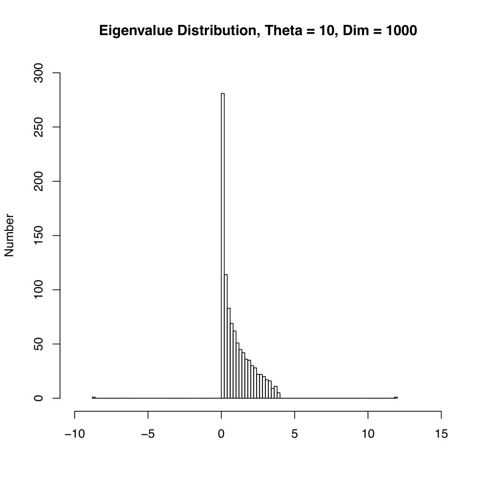 Figure 1
Peer Reviews
No public reviews on file for this paper yet. If you reviewed it on a platform where reviews are public (OpenReview, ICLR, NeurIPS, ICML), you can paste yours below so the community can read it here.
Videos
No videos yet. Explain this paper in a talk, walkthrough, or lecture? Add one.
On the
outlying eigenvalues of a polynomial in large independent random matrices
Serban T. Belinschi
Institut de Mathématiques de Toulouse; UMR5219; Université de Toulouse; CNRS; UPS, F-31062 Toulouse, FRANCE
,
Hari Bercovici
Department of Mathematics and Statistics, Indiana University, Bloomington, IN 47405 U.S.A.
and
Mireille Capitaine
Institut de Mathématiques de Toulouse; UMR5219; Université de Toulouse; CNRS; UPS, F-31062 Toulouse, FRANCE
Abstract.
Given a selfadjoint polynomial in two noncommuting selfadjoint indeterminates, we investigate the asymptotic eigenvalue behavior of the random matrix , where and are independent Hermitian random matrices and the distribution of is invariant under conjugation by unitary operators. We assume that the empirical eigenvalue distributions of and converge almost surely to deterministic probability measures and , respectively. In addition, the eigenvalues of and are assumed to converge uniformly almost surely to the support of and respectively, except for a fixed finite number of fixed eigenvalues (spikes) of . It is known that almost surely the empirical distribution of the eigenvalues of converges to a certain deterministic probability measure (sometimes denoted ) and, when there are no spikes, the eigenvalues of converge uniformly almost surely to the support of . When spikes are present, we show that the eigenvalues of still converge uniformly to the support of , with the possible exception of certain isolated outliers whose location can be determined in terms of , and the spikes of . We establish a similar result when is replaced by a Wigner matrix. The relation between outliers and spikes is described using the operator-valued subordination functions of free probability theory. These results extend known facts from the special case in which .
HB was supported by a grant from the National Science Foundation. This work was started while HB was visiting the Institute of Mathematics of Toulouse as Professeur Invité.
1. Introduction
Let and be two Borel probability measures with bounded support on . Suppose given, for each positive integer , selfadjoint independent random matrices and , with the following properties:
- (a)
the distribution of is invariant under conjugation by unitary matrices; 2. (b)
the empirical eigenvalue distributions of and converge almost surely to and , respectively; 3. (c)
the eigenvalues of and converge uniformly almost surely to the supports of and , respectively, with the exception of a fixed number of spikes, that is, fixed eigenvalues of that lie outside the support of .
When spikes are absent, that is, when , it was shown in [23] that the eigenvalues of converge uniformly almost surely to the support of the free additive convolution . When , the eigenvalues of also converge uniformly almost surely to a compact set such that and has no accumulation points in . Moreover, if , then is one of the spikes of , where is a certain subordination function arising in free probability. The relative position of the eigenvectors corresponding to spikes and outliers is also given in terms of subordination functions. We refer to [11] for this result.
Our purpose is to show that analogous results hold when the sum is replaced by an arbitrary selfadjoint polynomial . Then, by a comparison procedure to the particular case when is a G.U.E. (Gaussian unitary ensemble), we are also able to identify the outliers of an arbitrary selfadjoint polynomial when is a Wigner matrix independent from . This extends an earlier result [22] pertaining to additive deformations of Wigner matrices. More precisely we consider a Hermitian matrix , where is an infinite array of random variables such that
- (X0)
is independent from , 2. (X1)
, , , are independent, centered with variance 1, 3. (X2)
there exist , , and a random variable with finite fourth moment such that
[TABLE] 4. (X3)
Remark 1.1**.**
The matrix is called a G.U.E. if the variables , , and , are independent standard Gaussian. Assumptions (X2) and (X3) obviously hold if these variables are merely independent and identically distributed with a finite fourth moment.
Our result lies in the lineage of recent, and not so recent, works [5, 7, 8, 14, 18, 19, 21, 22, 26, 27, 31, 33, 35, 39, 40, 41] studying the influence of additive or multiplicative perturbations on the extremal eigenvalues of classical random matrix models, the seminal paper being [7], where the so-called BBP phase transition was observed.
We note that Shlyakhtenko [45] considered a framework which makes it possible to understand this kind of result as a manifestation of infinitesimal freeness. In fact, the results of [45] also allow one to detect the presence of spikes from the behaviour of the bulk of the eigenvalues of , even when has no outlying eigenvalues. In a related result, Collins, Hasebe and Sakuma [24] study the ‘purely spike’ case in which and the eigenvalues of and accumulate to given sequences and of real numbers converging to zero.
2. Notation and preliminaries on strong asymptotic freeness
We recall that a -probability space is a pair , where is a -algebra and is a state on . We always assume that is faithful. The elements of are referred to as random variables.
If is a classical probability space, then is a -probability space, where is the usual expected value. Given , is a -probability space, where denotes the normalized trace. More generally, if is an arbitrary -probability space and , then becomes a -probability space with the state .
The distribution of a selfadjoint element in a -probability space is a compactly supported probability measure on , uniquely determined by the requirement that , . The spectrum of an element is
[TABLE]
For instance, if is a selfadjoint matrix, then the distribution of relative to is the measure , where is the list of the eigenvalues of , repeated according to multiplicity. As usual, the support of a Borel probability measure on is the smallest closed set with the property that . It is known that if and is faithful, then In the following, we assume that is a tracial state, that is, .
Suppose that we are given -probability spaces and selfadjoint elements , . We say that converges in distribution to if
[TABLE]
We say that converges strongly in distribution to (or to ) if, in addition to (2.1), the sequence converges to in the Hausdorff metric. This condition simply means that for every there exists such that
[TABLE]
and
[TABLE]
for every . If all the traces are faithful, strong convergence can be reformulated as follows:
[TABLE]
for every polynomial with complex coefficients. This observation allows us to extend the concept of (strong) convergence in distribution to -tuples of random variables, . For every , we denote by the algebra of polynomials with complex coefficients in noncommuting indeterminates . This is a -algebra with the adjoint operation determined by
[TABLE]
Suppose that is a sequence of -probability spaces, , and is a sequence of -tuples of selfadjoint elements. We say that converges in distribution to if
[TABLE]
We say that converges strongly in distribution to if, in addition to (2.2), we have
[TABLE]
The above concepts extend to -tuples which do not necessarily consist of selfadjoint elements. The only change is that one must use polynomials in the variables and their adjoints , .
Remark 2.1**.**
Suppose that all the states , are faithful. As seen in [23, Proposition 2.1], converges strongly in distribution to if and only if converges strongly in distribution to for every selfadjoint polynomial Moreover, strong convergence in distribution also implies strong convergence at the matricial level. The following result is [36, Proposition 7.3].
Proposition 2.2**.**
Let be -probability spaces with faithful states , let , and let be a sequence of -tuples of selfadjoint elements . Suppose that converges strongly in distribution to . Then for every and every matrix polynomial .
A special case of strong convergence in distribution arises from the consideration of random matrices in . The following result follows from [23, Theorem 1.4] and [12, Theorem 1.2].
Theorem 2.3**.**
Let denote the space , . Suppose that are fixed, , and are mutually independent random tuples of matrices in some classical probability space such that:
- (i)
* are independent unitaries distributed according to the Haar measure on the unitary group .*
- (ii)
* are independent Hermitian matrices, each satisfying assumptions and in the introduction.*
- (iii)
* is a vector of selfadjoint matrices such that the sequence converges strongly almost surely in distribution to some deterministic -tuple in a -probability space.*
Then there exist a -probability space , a free family of Haar unitaries, a semicircular system and , such that, and are free and converges strongly almost surely in distribution to .
We recall that a tuple of elements in a -probability space is called a semicircular system if is a free family of selfadjoint random variables, and for every , is the standard semicircular distribution defined by
[TABLE]
An element is called a Haar unitary if and for all . Note that Theorem 1.2 in [12] deals with deterministic but the random case readily follows as pointed out by assertion 2 in [36, Section 3]. The point of Theorem 2.3 is, of course, that the resulting convergence is strong. Convergence in distribution was established earlier (see [49], [25], [3, Theorem 5.4.5]).
We also need a simple coupling result from [23, Lemma 5.1].
Lemma 2.4**.**
Suppose given selfadjoint matrices , , such that the sequences and converge strongly in distribution. Then there exist diagonal matrices , , such that , , and the sequence converges strongly in distribution.
3. Description of the models
In order to describe in detail our matrix models, we need two compactly supported probability measures and on , a positive integer , and a sequence of fixed real numbers in . The matrix is random selfadjoint for all and satisfies the following conditions:
- (A1)
almost surely, the sequence converges in distribution to ,
- (A2)
are eigenvalues of , and
- (A3)
the other eigenvalues of , which may be random, converge uniformly almost surely to : almost surely, for every there exists such that
[TABLE]
In other words, only the eigenvalues prevent from converging strongly in distribution to .
We investigate two polynomial matricial models, both involving . The first model involves a sequence of random Hermitian matrices such that
- (B0)
is independent from ,
- (B1)
converges strongly in distribution to the compactly supported probability measure on ,
- (B2)
for each , the distribution of is invariant under conjugation by arbitrary unitary matrices.
The matricial model is
[TABLE]
for an arbitrary selfadjoint polynomial .
The second model deals with random Hermitian Wigner matrices , where is an infinite array of random variables satifying conditions in the introduction. The matricial model is
[TABLE]
for an arbitrary selfadjoint polynomial .
In the discussion of the first model, we use results of Voiculescu [49] (see also [54]), who showed that there exist a free pair of selfadjoint elements in a II1-factor such that, almost surely, the sequence converges in distribution to . Thus, , and the sequence converges in distribution to (that is,
[TABLE]
in the weak∗ topology) for every selfadjoint polynomial . When , Lemma 2.4, Theorem 2.3 and Remark 2.1, show that, almost surely, this convergence is strong (see the proof of Corollary 2.2 in [23]).
For the second model we use [12, Proposition 2.2] and [3, Theorem 5.4.5], where it is seen that for every selfadjoint polynomial we have
[TABLE]
almost surely in the weak∗ topology, where and are freely independent selfadjoint noncommutative random variables, , and . As in the first model, Theorem 2.3 and Remark 2.1 show that, almost surely, the sequence converges strongly in distribution to provided that .
Our main result applies, of course, to the case in which . Let be either or . The set of outliers of is calculated from the spikes using Voiculescu’s matrix subordination function [52]. When , we also show that the eigenvectors associated to these outlying eigenvalues have projections of computable size onto the eigenspaces of corresponding to the spikes. The precise statements are Theorems 6.1 and 6.3. Sections 4 and 5 contain the necessary tools from operator-valued noncommutative probability theory while Sections 7–10 are dedicated to the proofs of the main results.
4. Linearization
As in [4, 13], we use linearization to reduce a problem about a polynomial in freely independent, or asymptotically freely independent, random variables, to a problem about the addition of matrices having these random variables as entries. Suppose that . For our purposes, a linearization of is a linear polynomial of the form
[TABLE]
where is a complex variable, and
[TABLE]
with for some , and the following property is satisfied: given and elements in a -algebra , is invertible in if and only if is invertible in . Usually, this is achieved by ensuring that exists as an element of and is one of the entries of the . It is known (see, for instance, [42]) that every polynomial has a linearization. See [29] for earlier uses of linearization in free probability.
In the following we also say, more concisely, that is a linearization of . We also suppress the unit of the algebra when there is no risk of confusion. For instance, we may write in place of
We describe in some detail a linearization procedure from [4] (see also [34]) that has several advantages. In this procedure, we always have , where denotes the matrix whose only nonzero entry equals and occurs in the first row and first column. Given , we produce an integer and a linear polynomial of the form
[TABLE]
such that , , is an invertible matrix in whose inverse is a polynomial of degree less than or equal to the degree of , and . Moreover, if , the coefficients of can be chosen to be selfadjoint matrices in .
The construction proceeds by induction on the number of monomials in the given polynomial. If is a monomial of degree [math] or , we set and . If , where and , we set and
[TABLE]
As noted in [34], the lower right corner of this matrix has an inverse of degree in the algebra . (The constant term in this inverse is a selfadjoint matrix and its spectrum is contained in .) Suppose now that , where , and that linear polynomials
[TABLE]
with the desired properties have been found for and . Then we set and observe that the matrix
[TABLE]
is a linearization of with the desired properties. The construction of a linearization is now easily completed for an arbitrary polynomial. Suppose now that is a selfadjoint polynomial, so for some other polynomial . Suppose that the matrix
[TABLE]
of size is a linearization of . Then we set and observe that the selfadjoint linear polynomial
[TABLE]
linearizes . It is easy to verify inductively that this construction produces a matrix such that the constant term of has spectrum contained in . These properties of [34], and particularly the following observation, facilitate our analysis.
Lemma 4.1**.**
Let , and let
[TABLE]
be a linearization of as constructed above. There exist a permutation matrix and a strictly lower triangular matrix such that .
Proof.
We show that there exist a permutation matrix and a strictly lower triangular matrix permutation matrices such that . Then we can define and . The existence of and is proved by following inductively the construction of . If , , we define
[TABLE]
and let the only nonzero entries of be just below the main diagonal. If , and linearizations for and have been found, then the desired matrices are obtained simply by taking direct sums of the matrices corresponding to and . The case in which is treated similarly (different factorizations must be used for and ). ∎
Lemma 4.2**.**
Suppose that , and let
[TABLE]
be a linearization of with the properties outlined above. Then for every , and for every , we have
[TABLE]
where the sign is . Moreover,
[TABLE]
Proof.
Suppressing the variables , we have
[TABLE]
Lemma 4.1 implies that is and the determinant identity follows immediately. The dimension of the kernel of a square matrix does not change if the matrix is multiplied by some other invertible matrices. Also, since is invertible, the kernel of the matrix on the right hand side of the last equality is easily identified with . The last assertion follows from these observations. ∎
In the case of selfadjoint polynomials, applied to selfadjoint matrices, we can estimate how far is from not being invertible.
Lemma 4.3**.**
Suppose that , and let
[TABLE]
be a linearization of with the properties outlined above. There exist polynomials with nonnegative coefficients with the following property: given arbitrary selfadjoint elements in a unital -algebra , and given such that is invertible, we have
[TABLE]
In particular, given two real constants , there exists such that and imply .
Proof.
For every element of a -algebra, we have . Equality is achieved, for instance, if . A matrix calculation (in which we suppress the variables ) shows that
[TABLE]
The lemma follows now because the entries of , , and are polynomials in , and
[TABLE]
because is selfadjoint. ∎
The dependence on in the above lemma is given via the norms of and of . Since , we see that .
5. Subordination
Consider a von Neumann algebra endowed with a normal faithful tracial state , let be unital von Neumann subalgebras, and denote by the unique trace-preserving conditional expectation of onto (see [46, Proposition V.2.36]). Denote by the operator upper-half plane of : . Given two arbitrary selfadjoint elements , we define the open set to consist of those elements such that is invertible and is invertible as well. Then the function
[TABLE]
defined by
[TABLE]
is analytic. This equation can also be written as
[TABLE]
Properties (1), (2), and (3) in the following lemma are easy observations, while (4) follows as in [10, Remark 2.5].
Lemma 5.1**.**
Fix and as above. Then:
- (1)
The set is selfadjoint. 2. (2)
, 3. (3)
* and .* 4. (4)
, .
There is one important case in which takes values in , and thus (5.2) allows us to view as a subordination function in the sense of Littlewood. Denote by the connected component of that contains . The following basic result is from [48].
Theorem 5.2**.**
With the above notation, suppose that and are free over and is the unital von Neumann generated by and . Then
[TABLE]
In our applications, the algebra is (isomorphic to) for some . More precisely, let be a von Neumann algebra endowed with a normal faithful tracial state , and let . Then can be identified with the subalgebra of . Moreover, is endowed with the faithful normal tracial state , and is the trace-preserving conditional expectation from to . The following result is from [37].
Proposition 5.3**.**
Let be a von Neumann algebra endowed with a normal faithful tracial state , let be freely independent, let be a positive integer, and let . Then and are free over .
We show next how the spectrum of relates with the functions defined above. Thus, we fix and a linearization of as constructed in Section 4. Thus, are selfadjoint matrices for some . (Clearly unless .) Then we consider the random variables and in , the algebra , and ; clearly . We set
[TABLE]
and
[TABLE]
Thus,
[TABLE]
The left hand side of this equation is defined if for some , so it would be desirable that for such values of . This is not true except for special cases. (One such case applies to if is a semicircular variable free from [16, 9].) The following lemma offers a partial result.
Lemma 5.4**.**
With the notation above, there exists depending only on , , and such that if . The analytic function satisfies the equation for .
Proof.
Define an analytic function by
[TABLE]
We show that is invertible if is sufficiently large. Suppressing the variables and from the notation, it follows from the factorization used in the proof of Lemma 4.2 that
[TABLE]
Moreover, because of the matrix structure of , this matrix can be obtained by applying entrywise. According to the Schur complement formula, a matrix is invertible if both and are invertible. For our matrix, we have . The fact that for implies that is invertible. Next, we see that and are comparable to and , respectively. Using these estimates, one sees also that , so the invertibility of would follow from the invertibility of for large . Since
[TABLE]
we only need to verify that is invertible. Write as in Lemma 4.1. We have
[TABLE]
and is strictly lower triangular. The invertibility of follows. The quantities and can be estimated using only , , and , and this shows that can be chosen as a function of these objects. The last assertion of the lemma is immediate. ∎
The estimates in the preceding proof apply, by virtue of continuity, to nearby points in . We record the result for later use.
Corollary 5.5**.**
Let and be as in Lemma 5.4 and let . Then there exist a constant and a neighborhood of , depending only on , and , such that and for .
In some cases of interest, the analytic function extends to the entire upper and lower half-planes. We recall that a function defined in a domain with values in a Banach space is said to be meromorphic if, for every , the function is analytic in a neighborhood of for sufficiently large . For instance, if is a finite dimensional Banach algebra and is an analytic function such that is invertible for some , then the function is meromorphic in . This fact follows easily once we identify with an algebra of matrices, so the inverse can be calculated using determinants.
Lemma 5.6**.**
The function defined in Lemma 5.4 is meromorphic in .
Proof.
The lemma follow immediately from the observation preceding the statement applied to the function defined in (5.3) which is analytic in since, by hypothesis and by Theorem 5.2, takes values in a finite dimensional algebra. ∎
The conclusion of the preceding lemma applies, for instance, when with the usual trace . This situation arises in the study of random matrices. The function is also meromorphic provided that and are free random variables and . Since , we have .
Lemma 5.7**.**
If and are free and , then the function defined in Lemma 5.4 is meromorphic in with values in . Moreover, given an arbitrary , the function extends analytically to .
Proof.
Theorem 5.2 shows that takes values in . We have established that the domain of contains for sufficiently large . Fix a character of the commutative -algebra and denote by the algebra homomorphism obtained by applying to each entry. Using the notation (5.3), we have
[TABLE]
for sufficiently large . It follows immediately that the function
[TABLE]
is a meromorphic continuation of to . Moreover, the equation
[TABLE]
holds for large values and hence it holds on the entire domain of analyticity of . It follows that contains whenever is not a pole of , and for such values of . To verify the last assertion, choose such that and apply to (5.4) to obtain
[TABLE]
Thus is an analytic extension of to . ∎
6. Main results and example
Fix a polynomial and choose, as in Section 4, a linearization of of the form , where . In particular, are selfadjoint matrices.
Suppose that and are two sequences of selfadjoint random matrices satisfying the hypotheses (A1)–(A3) and (B0)–(B2) of Section 3. As noted earlier, the pairs in converge almost surely in distribution to a pair of freely independent selfadjoint random variables in a -probability space such that and . By Theorem 5.2, there exists a selfadjoint open set , and an analytic function such that
[TABLE]
As shown in Lemma 5.7, the map
[TABLE]
is meromorphic on . Define a new function
[TABLE]
It follows from Lemma 5.1 that continues analytically to a neighbourhood of . (Indeed, is bounded near every pole of .) Define
[TABLE]
and denote by the order of as a zero of at . Also set for , and note that is an isolated set in . With this notation, we are ready to state our first main result. The notation indicates the spectral measure of the matrix , that is, is the orthogonal projection onto the linear span of the eigenvectors of corresponding to eigenvalues in the Borel set .
Theorem 6.1**.**
(1)* Suppose that . Then there exists such that for every , almost surely for large , the random matrix has exactly eigenvalues in the interval , counting multiplicity.*
(2)* Suppose in addition that the spikes of are distinct and . Then, for small enough, almost surely*
[TABLE]
where is the residue of the meromorphic function at .
Remark 6.2**.**
If we know in addition that is analytic at the point , then the function can be replaced by In that case, is equal to the multiplicity of as a zero of
[TABLE]
This situation arises, for instance, when is a semicircular variable and it is relevant when is replaced by a Wigner matrix . Under the hypotheses of Section 3, we obtain the following result. Note that the subordination function has the more explicit form
[TABLE]
Theorem 6.3**.**
Let and be free selfadjoint elements in a -probability space with distribution and respectively see (2.3), , and let be defined as in Remark 6.2. Then, for sufficiently small , almost surely for large , there are exactly eigenvalues of in an -neighborhood of .
Remark 6.4**.**
The subordination function can be calculated more explicitly if (and hence ). In this case,
[TABLE]
As an illustration, consider the random matrix
[TABLE]
where is a standard G.U.E. matrix of size (thus, each entry of has unit norm in ) and
[TABLE]
In this case, has rank one, and thus . It follows that the limit spectral measure of is the same as the limit spectral measure of . Thus, is the Marchenko-Pastur distribution with parameter 1:
[TABLE]
The polynomial is , , and is the standard semi-circular distribution. An economical linearization of is provided by , where
[TABLE]
Denote by
[TABLE]
the Cauchy transform of the measure . (The branch of the square root is chosen so for .) This function satisfies the quadratic equation . Suppose now that . Denoting by the usual expectation and using Remark 6.4, we have
[TABLE]
The inverse of is then calculated explicitly and application of the expected value to its entries yields eventually
[TABLE]
After calculation, the equation reduces to
[TABLE]
This equation has two solutions, namely
[TABLE]
one of which is negative. The positive solution belongs to precisely when . Thus, the matrix exhibits one (negative) outlier when and two outliers (one negative and one ) when . The second situation is illustrated by the simulation presented in Figure 1.
7. Outline of the proofs
We consider first the matricial model (3.1), that is, , where and are independent and the distribution of is invariant under unitary conjugation. As seen in [23, Proposition 6.1], can be written as almost surely, where is distributed according to the Haar measure on the unitary group , is a diagonal random matrix, and is independent from . As pointed out in [36, Section 3, Assertion 2], it suffices to prove Theorem 6.1 under the assumption that and are constant selfadjoint matrices that can be taken to be diagonal in the standard basis. Thus, we work with
[TABLE]
and
[TABLE]
where , and is uniformly distributed in .
Similarly, the proof for the second model reduces to the special case in which is a constant matrix.
Choose a linearization of as in Section 4. In the spirit of [14], the first step in the proofs of Theorems 6.1 and 6.3 consists of reducing the problem to the convergence of random matrix function of fixed size , involving the generalized resolvent of the linearization applied to . For the first model, this convergence is established in Section 8 by extending the arguments of [11] and making use of the properties of the operator-valued subordination function described in Section 5. For the second model, the convergence of is obtained in Section 10 via a comparison with the G.U.E. case. The case in which is a G.U.E. is, of course, a particular case of the unitarily invariant model.
8. Expectations of matrix-valued random analytic maps
As seen earlier in this paper, it suffices to prove Theorem 6.1 in the special case in which the matrix is constant and is a random unitary conjugate of another constant matrix. In this section, we establish some useful ingredients specific to this situation. We fix sequences and , where , and a sequence of random matrices such that is uniformly distributed in the unitary group . We also fix a selfadjoint polynomial and a selfadjoint linearization
[TABLE]
of as in Section 4. The random variables and are viewed as elements of the noncommutative probability space , where and . For every we consider the elements , and the algebras and , both identified with subalgebras of . The conditional expectation is simply the expected value and it is accordingly denoted . We use the notation
[TABLE]
Recall that consists of those matrices with the property that is invertible in and is invertible in . In particular, if then the matrix is invertible for every . The set is open and it contains . According to Lemma 5.6 and the remarks following it, the function is meromorphic in .
For simplicity of notation, we write
[TABLE]
and observe that is an element of , that is, a random matrix of size . We also write
[TABLE]
for sample values of this random variable. The function is given by
[TABLE]
We start by showing that the matrix has a block diagonal form, thus extending [11, Lemma 4.7]. We recall that the commutant and double commutant of a set are denoted by and , respectively. We use the fact that . If then is the linear span of the matrices . In particular, every eigenvector of is a common eigenvector for the elements of .
For each , we select an eigenbasis for the operator and denote by the corresponding eigenvalues, that is, . We write for the orthogonal projection onto the space generated by , . Thus, the double commutant is contained in the linear span of .
We write for the commutator of two elements in an algebra.
Lemma 8.1**.**
For every we have:
- (1)
. In particular, there exist analytic functions , , such that
[TABLE]
- (2)
For every ,
[TABLE]
Proof.
The first assertion in (1) follows from an application of (2) to an arbitrary matrix and from the fact that . The second assertion follows because we also have . To prove (2), observe that the analytic map
[TABLE]
is defined for in an open neighbourhood of the set of selfadjoint matrices in . The unitary invariance of implies that if is selfadjoint. Since the selfadjoint matrices form a uniqueness set for analytic functions, we conclude that is constant on an open subset of containing the selfadjoint matrices. Given an arbitrary , we conclude that the function is defined and constant for with sufficiently small. Differentiate with respect to and set , we obtain
[TABLE]
The equality
[TABLE]
applied in the relation above, yields (2). ∎
The following result is simply a reformulation of Lemma 8.1 that emphasizes the fact that the functions extend holomorphically to the open set
Corollary 8.2**.**
We have
[TABLE]
for every such that is invertible.
It is useful to rewrite assertion (2) of Lemma 8.1 as follows:
[TABLE]
This is analogous to [11, (4.10)] and the derivation is practically identical. Relation (8.4) allows us to estimate the differences between the matrices once we control the differences . For this purpose, we use the concentration of measure result in [3, Corollary 4.4.28]. This requires estimating the Lipschitz constant of the map (see (8.2)) in the Hilbert-Schmidt norm. We use the notation for the Hilbert-Schmidt norm of an arbitrary matrix .
Lemma 8.3**.**
Suppose that and . Then
[TABLE]
where .
Proof.
A simple calculation shows that
[TABLE]
Next we see that
[TABLE]
and thus
[TABLE]
Use now the equality to deduce that
[TABLE]
The lemma follows from this estimate. ∎
Proposition 8.4**.**
Suppose that , , and moreover,
[TABLE]
Let be matrices of norm one and rank uniformly bounded by . Then:
- (1)
Almost surely,
[TABLE]
- (2)
There exists such that
[TABLE]
In particular, there exists a dense countable subset such that almost surely, (8.5) holds for any .
Proof.
An arbitrary operator of rank can be written as a sum of operators of rank one (with the same or smaller norm). Thus we may, and do, restrict ourselves to the case in which the operators and are projections of rank . In this case, is a scalar multiple of a fixed operator of rank one and Lemma 8.3 shows that this function satisfies a Lipschitz estimate. This estimate, combined with [3, Corollary 4.4.28], shows that
[TABLE]
for every and every . The hypothesis implies that the last denominator has a bound independent of . Part (1) of the lemma follows from this inequality, while (2) follows from the formula , valid for arbitrary random variables . ∎
Remark 8.5**.**
While Proposition 8.4 was formulated for , the hypothesis (and therefore the conclusion of the proposition) is also satisfied in the following cases:
- (1)
with ;
- (2)
with , by an estimate provided by Lemma 4.3;
- (3)
with , by the same estimate provided that
[TABLE]
Corollary 8.6**.**
Under the assumptions of Proposition 8.4 suppose that we also have and set
[TABLE]
Let be a compact set. Then, almost surely, the functions
[TABLE]
converge to zero uniformly on as .
Proof.
According to Proposition 8.4 and Remark 8.5(2) and (3), almost surely, for every such that and , we have pointwise convergence to zero. A second application of Remark 8.5 yields uniform bounds on for all of these functions, and this implies uniform convergence because the resolvents involved are analytic in . ∎
We apply the concentration results just proved to operators and , of the form , where are the projections used in Lemma 8.1. The rank of is equal to .
Proposition 8.7**.**
Suppose that and let be such that
[TABLE]
and
[TABLE]
Then .
Proof.
The conclusion of the propostion is equivalent to
[TABLE]
as . Fix and set . Thus, is an operator of rank one such that for every . We have
[TABLE]
and, similarly,
[TABLE]
Next, we apply (8.4) and use the fact that commutes with . Setting , , we obtain
[TABLE]
Since , an application of the Cauchy-Schwarz inequality leads to the following estimate:
[TABLE]
We have and the product of the last two factors above is estimated via (8.6) by with independent of . Thus,
[TABLE]
with independent of and . The lemma follows. ∎
In the probability model we consider, the sequences and are uniformly bounded in norm and, in addition, the sequences and converge weakly to and , respectively. We denote by a pair of free random variables in some -probability space such that the sequence converges in distribution to . We also set
[TABLE]
In other words, is the usual matrix subordination function associated to the pair .
Proposition 8.8**.**
Suppose that and that the sequence converges to in distribution. Let be a connected open set containing and such that the sequence of functions is locally uniformly bounded on . Then
[TABLE]
Proof.
By hypothesis, the analytic functions form a normal family on . By Proposition 8.7, it suffices to prove that every subsequential limit of this sequence equals . Suppose that converges on to a function . Fix such that . Then
[TABLE]
and thus
[TABLE]
Setting , letting , and observing that the series on the right is uniformly dominated, we conclude that
[TABLE]
The fact that the pairs converge to implies that
[TABLE]
Thus, we obtain the equality
[TABLE]
and this easily yields . Since is connected, we must have , thus concluding the proof. ∎
Corollary 5.5 implies the following result.
Corollary 8.9**.**
Suppose that and the sequence converges to in distribution. Let where is the constant provided by Lemma 5.4. Then, for every , we have and
[TABLE]
The preceding results combine to yield convergence results for sample resolvents. For the following statement, it is useful to identify with a subspace of if and to denote by the standard basis in . Thus, we have provided that .
Proposition 8.10**.**
Suppose that and that the sequence converges to in distribution. Suppose also that is diagonal in the standard basis, that is, , , and that is such that the limits exist for . Denote by the orthogonal projection onto , . Let be a connected open set containing and such that the sequence of functions is locally uniformly bounded on . Then almost surely
[TABLE]
in the norm topology for every .
Proof.
By Proposition 8.4, it suffices to show that the conclusion holds with in place of . We observe that
[TABLE]
so the desired conclusion follows from Proposition 8.8. ∎
We observe for use in the following result that there exists a domain as in the above statement such that for every .
When the convergence of to is strong, the preceding result extends beyond . In this case, converges almost surely to and thus the sample resolvent is defined almost surely for large even for . We also recall that the function
[TABLE]
extends analytically to if . These analytic extensions are used in the following statement.
Proposition 8.11**.**
Under the hypothesis of Proposition 8.10, suppose that the pairs converge strongly to . Then almost surely
[TABLE]
for , . The convergence is uniform on compact subsets of .
Proof.
Strong convergence implies that for , so the functions extend analytically to . Let be a connected open set containing which is at a strictly positive distance from . We prove that the conclusion of the proposition holds for provided that is such that the conclusion of Corollary 8.6 holds and for and sufficiently large . By hypothesis, the collection of such points has probability . Lemma 4.3 shows that the family of functions is locally uniformly bounded on for large . By Montel’s theorem, we can conclude the proof by verifying the conclusions of the proposition for with . For such values of , the result follows from Proposition 8.10. ∎
9. The unitarily invariant model
In this section we prove Theorem 6.1 under the additional condition that is a constant matrix and is a random unitary conjugate of another constant matrix. We may, and do, assume that for , is diagonal in the standard basis with eigenvalues and, as before, . Then the random matrices and are viewed as elements of the noncommutative probability space . We fix free selfadjoint random variables in some tracial -probability space such that the pairs converge in distribution to as . This convergence is not strong because of the spikes . As in [11], we consider closely related pairs that do converge strongly to . Namely, we set , where is diagonal in the standard basis of with eigenvalues that coincide with those of except that is an arbitrary (but fixed for the remainder of this section) element of . For , the difference can then be written as , where is the diagonal matrix with eigenvalues and is the orthogonal projection.
According to Lemma 4.2, and have the same dimension for every . Setting , strong convergence of the pairs implies that almost surely the sample resolvent is defined for sufficiently large if . (We continue using the notation introduced in (8.1), (8.2), and (8.3).) We need to consider the matrix
[TABLE]
since the order of as a zero of its determinant equals , and hence the number of eigenvalues of in a neighborhood of a given is the number of zeros of this determinant in . Thus, we need to consider the zeros in of
[TABLE]
Using Sylvester’s identity ( if is an matrix and is a matrix) and the fact that , this determinant can be rewritten as
[TABLE]
At this point, we observe that the hypothesis of Proposition 8.11 are satisfied with . We conclude that almost surely
[TABLE]
where
[TABLE]
and the convergence is uniform on compact sets. The limit is a (deterministic) analytic function on . An application of Hurwitz’s theorem on zeros of analytic functions (see [1, Theorem 5.2]) yields the following result.
Proposition 9.1**.**
Suppose that , , , for , and the function has at most one zero in the interval . Then, almost surely for large , the matrix has exactly eigenvalues in the interval , where is the order of as a zero of and if this function does not vanish on .
Part(1) of Theorem 6.1 is a reformulation of Proposition 9.1. To see that this is the case, we observe that is a diagonal matrix and thus the matrix
[TABLE]
is block diagonal with diagonal blocks
[TABLE]
If has a zero of order at then the number in the statement is . We recall that is analytic on but is only meromorphic. It is not immediately apparent that the number does not depend on but this is a consequence of the following result.
Lemma 9.2**.**
Suppose that are such that extends analytically to for . Then the order of as a zero of
[TABLE]
does not depend on .
Proof.
An easy calculation shows that
[TABLE]
The desired conclusion follows if we prove that the function
[TABLE]
is analytic and invertible at . We have
[TABLE]
and
[TABLE]
so the analyticity and invertibility of follow from the hypothesis. ∎
We proceed now to Part(2) of Theorem 6.1. Thus, assumptions (A1–A3) and (B0–B2) are in force and, in addition, the spikes are distinct. In particular, .
If is a Borel set and is a selfadjoint operator, then denotes the orthogonal projection onto the linear span of the eigenvectors of corresponding to eigenvalues in . For instance, under the hypotheses of Part(2) of Theorem 6.1, is a projection of rank one for . If is a continuous function, then denotes the usual functional calculus for selfadjoint matrices. Thus, if for some and , then .
Fix and small enough. We need to show that, almost surely,
[TABLE]
Choose and such that , for and . Pick infinitely differentiable functions supported in such that , . Also pick an infinitely differentiable function supported in such that is identically on . Then part (1) of Theorem 6.1 implies that, almost surely for large , we have
[TABLE]
In anticipation of a concentration inequality, we prove a Lipschitz estimate for the functions defined by
[TABLE]
Lemma 9.3**.**
There exists , independent of , such that
[TABLE]
Proof.
Given a Lipschitz function , we denote by the smallest constant such that
[TABLE]
and we set . If are two Lipschitz functions, then and
[TABLE]
Since the functions and are Lipschitz with constant , we deduce immediately that the map is Lipschitz with constant bounded independently of . It is well-known that a Lipschitz function is also Lipschitz, with the same constant, when viewed as a map on the selfadjoint matrices with the Hilbert-Schmidt norm (see for instance, [18, Lemma A.2]). The function is infinitely differentiable with compact support, hence Lipschitz. We deduce that the map is Lipschitz with constant bounded independently of . Finally, we have
[TABLE]
and the lemma follows because . ∎
An application of [3, Corollary 4.4.28] yields
[TABLE]
and the Borel-Cantelli lemma shows that, almost surely,
[TABLE]
The expected value in (9.2) is estimated using [18, Lemma 6.3] and the fact that is the projection onto the th coordinate. If we set and , , then
[TABLE]
The construction of the linearization (Section 4) is such that the matrix , viewed as an block matrix, has as its entry. By Propositions 8.4(1) and 8.10 (with in place of ) and the unitary invariance of the distribution of , for the matrices
[TABLE]
converge as to the block diagonal matrix with diagonal entries
[TABLE]
It follows that
[TABLE]
We intend to let in (9.3) using (9.4), so we consider the differences
[TABLE]
By Corollary 5.5, these functions are defined on for some and satisfy . We claim that there exists a sequence such that and
[TABLE]
To verify this claim, we observe first [2] that the function is the Cauchy-Stieltjes transform of a Borel probability measure on . Since
[TABLE]
the measures have uniformly bounded supports. Now, (9.4) shows that the Cauchy-Stieltjes transform of any accumulation point of this sequence of measures is equal to . It follows that this sequence has a weak limit that is a Borel probability measure with compact support. The existence of the sequence follows from [11, Lemma 4.1] applied to the signed measures .
We use (9.5), (9.3), and the Lemma from [20, Appendix] to obtain
[TABLE]
The choice of , and the fact that
[TABLE]
is analytic and real-valued on the intervals and , imply that the last line in (9.6) can be rewritten as
[TABLE]
Recall (see, for instance, [1, Chapter 4]) that if is an analytic function on a simply connected domain , except for an isolated singularity , then . Here is a closed Jordan path in not containing , is the winding number of with respect to , and is that number which satisfies the condition that has vanishing period (called the residue of at ). Denote by the rectangle with corners and let be the boundary of oriented counterclockwise. The expression in (9.7) represents the integral of on the horizontal segments in . It is clear that the integral of on the vertical segments is , and thus (9.6) implies the equality
[TABLE]
The alternative formula in Theorem 6.1 follows from the fact that has a simple pole at because maps to .
10. The Wigner model
We proceed now to the proof of Theorem 6.3. The matrices are subject to the hypotheses (A1–A3), while and satisfies conditions (X0–X3). By [36, Section 3, Assertion 2], it suffices to proceed under the additional hypothesis that each is a constant matrix. The free variables and are such that has standard semicircular distribution .
One consequence of the fact that is a semicircular variable is that the function is analytic on the entire set
[TABLE]
This justifies the comment from Remark 6.2. We recall that in this special case the subordination function is given by
[TABLE]
Since the distribution of the random matrix is not usually invariant under unitary conjugation, we can no longer assume that is diagonal in the standard basis . There is however a (constant) unitary matrix such that is diagonal in the basis with eigenvalues , . Viewing each realization of the random matrices and as elements of the noncommutative probability space , almost surely the pairs converge in distribution, but not strongly, to as . A modification of provides almost surely strongly convergent pairs . Thus, let be diagonal in the basis with eigenvalues that coincide with those of except that is an arbitrary (but fixed for the remainder of this section) element of . For , the difference can then be written as , where is the diagonal matrix with eigenvalues and is the orthogonal projection. Almost surely, the pairs converge strongly to as shown in [12, Theorem 1.2] and [23, Proposition 2.1]. We continue using the notation introduced in (8.1) and (8.3) with and . The calculation in Section 9 show that, almost surely, for large enough, the number of eigenvalues of in a small enough neighborhood of is equal to the number of zeros of in this neighborhood, where
[TABLE]
is a random analytic function. We focus on the study of the large behavior of the matrix function
[TABLE]
We start with the special case in which is replaced by a standard G.U.E.. The following proposition is a consequence of the results in Section 9. Thus, suppose that is a sequence of standard G.U.E. ensembles and we set and
[TABLE]
Proposition 10.1**.**
We have
[TABLE]
for every .
Proof.
Since G.U.E. ensembles are invariant under unitary conjugation we may, and do, assume that for every . For every we have
[TABLE]
and the second term is at most . As shown by Bai and Yin [6], this number tends to zero as . To estimate the first term, we recall that , where is a random matrix uniformly distributed in and is a random diagonal matrix, independent from , whose empirical spectral measure converges almost surely to as . Thus, we can write
[TABLE]
[TABLE]
Proposition 8.10 can be applied for almost every and it shows that
[TABLE]
converges to . The proposition follows now from an application of the dominated convergence theorem. ∎
Passing to arbitrary Wigner matrices requires an approximation procedure from [12, Section 2]. For every , there exist random selfadjoint matrices such that
- (H1)
the variables , , , , , are independent, centered with variance and satisfy a Poincaré inequality with common constant ,
- (H2)
for every ,
[TABLE]
and almost surely for large ,
[TABLE]
Set
[TABLE]
and
[TABLE]
for . It readily follows that, almost surely for large ,
[TABLE]
Properties (H1) and (H2) imply that, for every ,
[TABLE]
[TABLE]
and for any ,
[TABLE]
where for , and denote the classical cumulants of and respectively, and denote the classical cumulants of (we set ).
We use the following notation for an arbitrary matrix :
[TABLE]
and
[TABLE]
where (resp. ) denotes the (resp. ) matrix whose unique nonzero entry equals 1 and occurs in row and column .
Proposition 10.2**.**
There exists a polynomial in one variable with nonnegative coefficients such that for all large , for every , for every , and for every deterministic such that and , we have
[TABLE]
and
[TABLE]
The proof uses a well-known lemma.
Lemma 10.3**.**
Let be a real-valued random variable such that . Let be a function whose first derivatives are continuous and bounded. Then,
[TABLE]
where are the cumulants of , , and only depends on .
Proof of Proposition 10.2.
Following the approach of [38, Ch. 18 and 19] we introduce the interpolation matrix , , and the corresponding resolvent
[TABLE]
We have
[TABLE]
[TABLE]
Define a basis of the real vector space of selfadjoint matrices in as follows:
[TABLE]
[TABLE]
[TABLE]
In the following calculation, we write simply in place of and in place of :
[TABLE]
Next, we apply Lemma 10.3 with for , , to each random variable in the set
[TABLE]
and to each in the set
[TABLE]
Setting now we have:
[TABLE]
where
[TABLE]
for some , while and are polynomials in and . In the following, may vary from line to line. It is clear that
[TABLE]
Next, and are a finite linear combinations of terms of the form
[TABLE]
where is some subset of , , and is a permutation of . The two following cases hold:
- •
, in which case Lemma 11.1 yields
[TABLE]
- •
, in which case Lemma 11.1 yields
[TABLE]
We see now that for . Finally, and are finite linear combinations of terms of the form
[TABLE]
where is some subset of , and is a permutation of . Lemma 11.1 shows that the norm of such a term can be estimated by
[TABLE]
It follows that for . The proposition follows. ∎
We show next that is close to its expected value. This result uses concentration inequalities in the presence of a Poincaré inequality. We recall that if the law of a random variable satisfies the Poincaré inequality with constant and , then the law of satisfies the Poincaré inequality with constant . Moreover, suppose that the probability measures on satisfy the Poincaré inequality with constants respectively. Then the product measure on satisfies the Poincaré inequality with constant . That is, if is an arbitrary differentiable function such that and its gradient are square integrable relative to , then
[TABLE]
Here (see [28, Theorem 2.5]).
We use the following concentration result (see [3, Lemma 4.4.3 and Exercise 4.4.5] or [32, Chapter 3]).
Lemma 10.4**.**
Let be a probability measure on which satisfies a Poincaré inequality with constant . Then there exist and such that, for every Lipschitz function on with Lipschitz constant , and for every , we have
[TABLE]
The following result is similar to Proposition 8.4(1).
Proposition 10.5**.**
Suppose that are contractions of uniformly bounded rank. Given and , almost surely
[TABLE]
Proof.
As in the proof of Proposition 8.4, it suffices to consider the case in which and are contractions of rank . Write as a sum of rank projections. Then the norm in the statement is at most equal to
[TABLE]
where each is a contraction of rank . Given a selfadjoint matrix , we set and . We have
[TABLE]
and thus
[TABLE]
An application of Lemma 10.4 and of the comment preceding it yield
[TABLE]
for every , with a constant that does not depend in or . The proposition follows by an application of the Borel-Cantelli lemma. ∎
Corollary 10.6**.**
For every and every we have, almost surely,
[TABLE]
Observe now that
[TABLE]
We let and then and apply (10.6), (10.14), Proposition 10.2, and Proposition 10.1 to obtain the following result.
Theorem 10.7**.**
For every we have, almost surely, when goes to infinity, .
Everything is now in place for completing the argument.
Proof of Theorem 6.3.
We noted earlier that is analytic in . For fixed , set and . According to Lemma 4.2, is invertible, and thus there exists such that
[TABLE]
Theorem 2.3 and Proposition 2.2 imply that, almost surely, for every complex polynomial in one variable we have
[TABLE]
Asymptotic freeness implies that almost surely, for every complex polynomial in one variable,
[TABLE]
Thus, denoting the Hausdorff distance by , we deduce that almost surely for large enough,
[TABLE]
Note that is selfadjoint. For an arbitrary , we have
[TABLE]
It follows from (10.15) that, almost surely for all large , if , then
[TABLE]
Moreover, denoting by the smallest singular value of an arbitrary matrix ,
[TABLE]
Thus, almost surely for all large , provided that , we have In other words, almost surely, the family is normal in a neighborhood of . According to Theorem 10.7, for any , almost surely converges towards . Set
[TABLE]
Almost surely for any such that and , converges towards . The Vitali-Montel convergence theorem implies that that almost surely converges towards a holomorphic function on and, in particular, converges for any such that towards .
Now, the Hurwitz theorem on zeros of analytic functions implies that, almost surely for large , the function has as many zeros in a neighborhood of as the function
[TABLE]
Now, note that
[TABLE]
and
[TABLE]
Therefore
[TABLE]
The theorem follows. ∎
11. Appendix
The following result is [12, Lemma 8.1].
Lemma 11.1**.**
For any matrix ,
[TABLE]
and for any fixed ,
[TABLE]
and
[TABLE]
where is defined by (10.8).
The reference list from the paper itself. Each links out to its DOI / PubMed record.
- 1[1] Lars V. Ahlfors. An Introduction to the Theory of Analytic Functions of One Complex Variable. Third Edition (1979) Mc Graw-Hill, Inc. New York.
- 2[2] Naum Ilich Akhieser, The classical moment problem and some related questions in analysis. Translated by N. Kemmer. Hafner Publishing Co., New York, 1965.
- 3[3] G. W. Anderson, A. Guionnet, and O. Zeitouni, An introduction to random matrices , Cambridge University Press, Cambridge, 2010.
- 4[4] G. W. Anderson, Convergence of the largest singular value of a polynomial in independent Wigner matrices . Ann. Probab. 41 (2013), 2103–2181.
- 5[5] Z. D. Bai and J. Yao, On sample eigenvalues in a generalized spiked population model, J. Multivariate Anal . 106 (2012), 167–177.
- 6[6] Z. D. Bai and Y. Q. Yin, Necessary and sufficient conditions for almost sure convergence of the largest eigenvalue of a Wigner matrix . Ann. Probab., 16(4), (1988), 1729–1741.
- 7[7] J. Baik, G. Ben Arous, and S. Péché, Phase transition of the largest eigenvalue for nonnull complex sample covariance matrices, Ann. Probab. 33 (2005), 1643–1697.
- 8[8] J. Baik and J. W. Silverstein, Eigenvalues of large sample covariance matrices of spiked population models, J. Multivariate Anal . 97 (2006), 1382–1408.