Multi-scale time-stepping in molecular dynamics
A.C. Maggs

TL;DR
This paper presents a novel multi-scale time-stepping algorithm for molecular dynamics that selectively freezes parts of the system without affecting the thermodynamic properties of the non-central variables, enabling focused and accurate simulations.
Contribution
It introduces a new multi-scale molecular dynamics method that preserves thermodynamic accuracy while allowing selective freezing of system components.
Findings
No approximations in thermodynamic behavior of frozen parts
Conserves Newtonian dynamics in the region of interest
Enables efficient simulation of complex systems
Abstract
We introduce a modified molecular dynamics algorithm that allows one to freeze the dynamics of parts of a physical system, and thus concentrate the simulation effort on selected, central degrees of freedom. This freezing, in contrast to other multi-scale methods, introduces no approximations in the thermodynamic behaviour of the non-central variables while conserving the Newtonian dynamics of the region of physical interest.
Click any figure to enlarge with its caption.
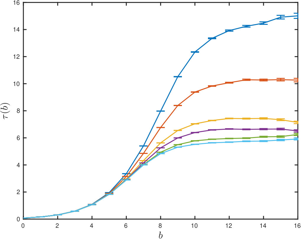 Figure 1
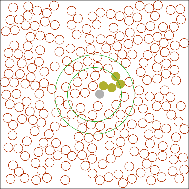 Figure 2
| deviation in | statistical error | |
|---|---|---|
| 2.5 | -0.0025 | |
| 3 | -0.0004 | |
| 4 | -0.0005 | |
| 5 | 0.0008 | |
| 6 | 0.0015 | |
| 8 | 0.0009 | |
| 10 | 0.0004 | |
| 0.001 |
Peer Reviews
No public reviews on file for this paper yet. If you reviewed it on a platform where reviews are public (OpenReview, ICLR, NeurIPS, ICML), you can paste yours below so the community can read it here.
Videos
No videos yet. Explain this paper in a talk, walkthrough, or lecture? Add one.
11institutetext: CNRS UMR7083, ESPCI Paris, PSL Research University, 10 rue Vauquelin, Paris, 75005, France
Molecular dynamics and particle methods Applications of Monte Carlo methods Computational methods in statistical physics and nonlinear dynamics
Multi-scale time-stepping in molecular dynamics
A.C. Maggs
Abstract
We introduce a modified molecular dynamics algorithm that allows one to freeze the dynamics of parts of a physical system, and thus concentrate the simulation effort on selected, central degrees of freedom. This freezing, in contrast to other multi-scale methods, introduces no approximations in the thermodynamic behaviour of the non-central variables while conserving the Newtonian dynamics of the region of physical interest.
pacs:
02.70.Ns
pacs:
02.70.Uu
pacs:
05.10.-a
Molecular dynamics simulation is the backbone of much numerical work in condensed matter physics and chemistry. It is formulated in terms of the underlying forces of the physical model and allows one to study thermodynamic and dynamic processes in microscopic detail. However, it is also clear that the method is, in some geometries, extravagantly wasteful. An important and obvious example occurs in biophysical applications where a single interesting complex is studied in the presence of a solvent: A solvated protein requires detailed simulation of large number of water molecules—in order to correctly hydrate the molecule, and also to separate periodic images in the simulation cell. Such systems seem to be obvious candidates for a multi-scale approach. Close to the protein all the dynamics are to be followed, but at larger distances from the protein the water molecules are spectators, which should give rise to self-averaging in large systems. Nevertheless, this “distant spectator” must be well modeled in order to limit finite size artefacts.
Such ideas have led to a number of interesting papers for the formulation of multiscale simulation [1, 2] where the spatial resolution of the solvent model changes as a function of position in the simulation cell. An alternative to this molecular coarse-graining is to use different integration methods in different regions using a simple, robust large-step integrator in the far field, coupled to more precise near field stepper, [3].
Another physical system where multi-scale ideas are important is in the modelling of deformations in solid materials. Here short-range atomistic modeling is coupled to larger scale continuum descriptions in order to reduce artefacts from the tiny samples that can be comfortably simulated [4, 5]. It is clear that careful matching is required to best interface the continuum and atomistic models.
The present paper introduces a complementary view on how to treat the far-field degrees of freedom. Rather than spatially coarse-graining or introducing continuum couplings we introduce a hierarchy in the speed of simulation. Central regions in the physical system advance with a full, molecular dynamic algorithm. Regions further away are regularly frozen so that on average time advances more slowly. However, the whole dynamic system is assembled in such a way that detailed-balance is obeyed; the entire simulated system thus samples the proper equilibrated thermodynamic ensemble. Thus there is no sharp boundary between interesting and spectator regions. All degrees of freedom are free to relax and fluctuate.
Physical intuition tells us that this can be potentially useful: In the simulation of water the dominant local process is Debye dielectric relaxation of the orientational dipole occurring on the scale of . In a long (micro-second simulation) simulation of a bio-molecule a single, distant water molecule influences, above all, due to the averaged, static dielectric properties which are fully developed at this tiny time scale. Putting more computational effort into this rotational process than is needed is clearly inefficient. The same can be said of a distant region in a simulation of mechanical deformation of a solid: full high statistics simulation of distant regions do not substantially increase the accuracy of the simulation of the near field.
We now consider the phase space dynamics of a system which has been partially frozen: To begin, consider the motion of a single particle with a reduced Hamiltonian which contains just that part of the full Hamiltonian that relate to the degree of freedom . We can study the evolution of the full canonical distribution with the reduced dynamics of only with the Poisson bracket:
[TABLE]
Generalising to a mixture of free and frozen particles we see that allowing a subsystem to evolve under the total potential energy of all the particles conserves the canonical distribution of the full system. At first examination this seems paradoxical. However, we note that the full phase space has independent directions. If we now allow evolution of part of a system to alternate with the full Hamiltonian dynamics this leads to motion in which certain cuts of phase space are explored quickly, while other cuts evolve slowly. Each possible dynamic process, however, fully conserves the desired measure.
The main trap in the imagined algorithm is the choice of particles in the near and far fields in a way that does not destroy detailed balance; this is the subject of the present paper. In the formulation of the algorithm we have been influenced by multi-scale Monte Carlo methods [6] for the simulation of simple fluids but also an elegant and efficient formulation of Zimm dynamics [7] as a multiscale problem. Both these methods move blocks of particles, while freezing the rest of the system. The originality of the present paper is the use of a molecular dynamics, rather than a Monte Carlo rule for the individual particle motions.
We note also that the ideas behind the algorithm are similar to a heat-bath algorithm which works by updating a small subpart of a physical system in a frozen background. Convergence to the Gibbs distribution requires only the use of detailed-balance in the local moves (or perhaps the even weaker criterion of balance [8]). Let us also note that there is a long tradition of combining molecular dynamics and Monte Carlo rules to produce more efficient algorithms [9, 10, 11, 12, 13, 14].
We now show how to implement the method, including the crucial choice of the partition between frozen and dynamic degrees of freedom. The implementation is based on a modified version of the leapfrog, or Verlet algorithm, well known for its excellent conserving properties. We define the operators for updating the velocities of particles, the positions of particles and for thermalising particles as follows:
[TABLE]
where, for simplicity we hide the vectorial nature of the update rules. denotes the temperature and a damping rate for velocity correlations due to interaction with a Langevin thermostat. The velocities, positions and forces are denoted respectively by , and . is a normally distributed random number with unit variance. We work with unit mass particles.
These individual steps are assembled into a time-reversible sequence [15]:
[TABLE]
Evolution for time steps gives the operator . The half step updates can be coalesced to give the thermalised leap-frog algorithm [16]. This defines a map on phase space compatible with detailed balance and the thermalised process converges to the canonical ensemble. We now add a further action in the dynamics. We stochastically displace (with probability ) a spherical barrier of radius : after application of the operator . This barrier, centred on the region of interest, has a radius drawn from a probability density
[TABLE]
The whole dynamic process then involves an alternation of microscopic leap-frog evolutions and barrier events:
[TABLE]
in manner which is still explicitly time reversible.
This barrier is selected with rather special properties. It does not interact with any particle in the system; the insertion has zero energy cost. However, the barrier changes the dynamics of the system strongly. All particles exterior to the barrier Fig. 1 are frozen in position. All particles within the barrier move in the total potential of the other interior particles plus the frozen exterior particles. When the radius of a barrier increases the particles restart their motion with exactly the same velocity they had before being frozen.
As stated this rule still has a major defect: particles in a time step can cross the barrier where their dynamic status becomes ambiguous. If they are then frozen the dynamics becomes irreversible since forwards and backwards motions are not generated in a manner compatible with detailed balance. We thus add one extra feature to the barrier — it acts as a perfect mirror to any incident interior particle. This reflecting barrier, together with the careful insertion of the barrier event within the half-step of the leap-frog method give rise to a dynamic system which is explicitly time reversible. Management of this extra dynamic process is treated using event-driven methods within the step [17]. If we take a particle which has bounced off the barrier in the time and reverse its speed it will backtrack on its own trajectory to within machine precision.
The probability distribution for the barrier gives with a preference for a radius which is close to . With this choice, eq. (1), the total numerical effort only increases very slowly (logarithmically) [6, 7] with the total system size: yet all particles move and relax during the simulation. As one goes away from the region of interest, the total simulation effort decreases.
We have thus a dynamic process on phase space respecting detailed balance, which in many ways is reminiscent of heat-bath Monte Carlo where a selected set of variables are re-sampled in the static background of the entire system. However, within the interior region of radius the particles always evolve under Newtonian dynamics. It is clear that the dynamics are not momentum conserving—collisions on the barrier act like a confining box. The method is thus unlikely to be useful in the case of physics dominated by long-ranged hydrodynamic interactions.
We applied the algorithm to the a simple two-dimensional Lennard-Jones fluid and studied the partial structure factors of a central region, and compared to a direct molecular dynamics simulation of the whole system. We use an integration time step , with damping in Lennard-Jones units and cut-off the interaction at . It was in this preliminary study that we became aware of the importance of the correct time-reversible version of the algorithm. Insert of the barrier in a non-symmetric postion in the standard leapfrog method led to a systematic deviation in measured correlations.
We then performed simulation with a short (5-mer) tethered polymer in a Lennard-Jones fluid, Fig. 1: Such small-scale simulation where very high statistics runs can be performed are those that are most sensitive to errors in the formulation of the algorithm. In the snapshot we draw two rings—the innermost corresponding to in Lennard-Jones units. The outer ring is the instantaneous position of the reflecting barrier chosen from the probability distribution eq. 1. We see the inner ring intercepts the chain. It is thus stochastically split between the mobile inside and the static outside region during its evolution. Despite this extreme perturbation to the dynamic the conformations of the chain are unperturbed. In Table 1 we report on the mean squared end-to-end separation, of the 5-mer as a function of the minimum barrier radius. We measure deviations in the polymer size, and give estimates of statistical errors.
We conclude that to a precision of better than 1 part in 2000 the mean-squared extension of the polymer is independent of . This requires simulations of length autocorrelation times. Note, that when we try simulating the polymer chain in small, periodic cells we see substantial modifications of the statistics of the chain when using cells of dimension with the smallest values of in Table 1.
We now study the autocorrelation dynamics of the chain using a method based on block averages [18], Fig. 2: A long time series with variance can be averaged into blocks of length , which themselves have an interblock variance . is the time in Lennard-Jones units between recordings in the time-series. If the blocks are longer than the integrated autocorrelation time, , we have . Thus as the block size increases an estimate of the autocorrelation time is
[TABLE]
When we plot this ratio as a function of it should plateau to a constant value, when the block size is longer than the autocorrelation time. In Fig. 2 this gives rise to a characteristic rising curve which encodes the autocorrelation dynamics of the chain. The value of the large plateau is then a true estimate of the integrated autocorrelation time. In the figure one can read-off the approximate autocorrelation time for several values . The highest curve, corresponding to the slowest relaxation, is for . We see that the dynamics has been strongly hindered due to the regular partition of the polymer between frozen and unfrozen zones. However, all the curves for are close, corresponding to the large system limit. Table 1 again shows that the dynamic process always generates the correct statistics of the chain, even if the parameters are chosen in such a way to strongly change the underlying dynamics.
We have demonstrated the possibility of embedding a full speed molecular dynamics simulation in a larger, more slowly evolving background in such a way that the whole system generates the canonical ensemble of the entire system. This gives essentially perfect boundary conditions for the simulation of the central region without having to build a coarse-grained model of the outside world, and without needing to couple a continuum theory.
We anticipate that such methods will be useful in the simulation of solvated molecules or in large scale simulation of elastic materials; in such systems much computational effort is lost in updating weakly interacting spectator molecules, rather than concentrating the computation effort on the specific object of interest. For use in situations where long-ranged interactions are important, as is the case with water one needs methods of evaluating efficiently the interactions in the presence of many frozen particles. One possibility is the use of a dynamic, propagative algorithm for the electrostatic field as has been presented in [19, 20, 21, 22].
In this paper we used a specific distribution for the barrier dimension eq. (1) which has been shown useful in Monte Carlo applications, but it is probable that the optimal distribution of work between near and far fields is problem dependent.
Acknowledgements.
We thank Ralf Everaers and Michael Schindler for extensive discussions on the formulation of multi-scale simulation methods.
The reference list from the paper itself. Each links out to its DOI / PubMed record.
- 1[1] \Name Potestio R., Español P., Delgado-Buscalioni R., Everaers R., Kremer K. Donadio D. \REVIEW Phys. Rev. Lett.1112013060601. http://link.aps.org/doi/10.1103/Phys Rev Lett.111.060601
- 2[2] \Name Potestio R., Fritsch S., Español P., Delgado-Buscalioni R., Kremer K., Everaers R. Donadio D. \REVIEW Phys. Rev. Lett.1102013108301. http://link.aps.org/doi/10.1103/Phys Rev Lett.110.108301
- 3[3] \Name Leimkuhler B. Matthews C. \REVIEW Proceedings of the Royal Society of London A: Mathematical, Physical and Engineering Sciences 4722016. http://rspa.royalsocietypublishing.org/content/472/2189/20160138
- 4[4] \Name Namilae S., Nicholson D. M., Nukala P. K. V. V., Gao C. Y., Osetsky Y. N. Keffer D. J. \REVIEW Phys. Rev. B 762007144111. http://link.aps.org/doi/10.1103/Phys Rev B.76.144111
- 5[5] \Name Karpov E., Yu H., Park H., Liu W. K., Wang Q. J. Qian D. \REVIEW International Journal of Solids and Structures 4320066359 . //www.sciencedirect.com/science/article/pii/S 0020768305005792
- 6[6] \Name Maggs A. C. \REVIEW Phys. Rev. Lett.972006197802. http://link.aps.org/doi/10.1103/Phys Rev Lett.97.197802
- 7[7] \Name Dyer O. T. Ball R. C. \Book Computationally efficient brownian dynamics via wavelet monte carlo (2016).
- 8[8] \Name Michel M., Kapfer S. C. Krauth W. \REVIEW The Journal of Chemical Physics 1402014054116. http://dx.doi.org/10.1063/1.4863991 · doi ↗