Three-body bound states with zero-range interaction in the Bethe-Salpeter approach
E. Ydrefors, J. H. Alvarenga Nogueira, V. Gigante, T. Frederico and, V.A. Karmanov
TL;DR
This paper solves the Bethe-Salpeter equation for three bosons with zero-range interactions, revealing regimes of unbound, bound, and unphysical states, and compares results with light-front calculations.
Contribution
First solution of the three-boson Bethe-Salpeter equation with zero-range interaction, including analysis of different binding regimes and comparison with light-front methods.
Findings
Identification of three interaction regimes: unbound, bound, and unphysical states.
Discovery of a deeply bound Borromean three-body state.
Relativistic three-body forces increase binding energy.
Abstract
The Bethe-Salpeter equation for three bosons with zero-range interaction is solved for the first time. For comparison the light-front equation is also solved. The input is the two-body scattering length and the outputs are the three-body binding energies, Bethe-Salpeter amplitudes and light-front wave functions. Three different regimes are analyzed: ({\it i}) For weak enough two-body interaction the three-body system is unbound. ({\it ii}) For stronger two-body interaction a three-body bound state appears. It provides an interesting example of a deeply bound Borromean system. ({\it iii}) For even stronger two-body interaction this state becomes unphysical with a negative mass squared. However, another physical (excited) state appears, found previously in light-front calculations. The Bethe-Salpeter approach implicitly incorporates three-body forces of relativistic origin, which are…
Click any figure to enlarge with its caption.
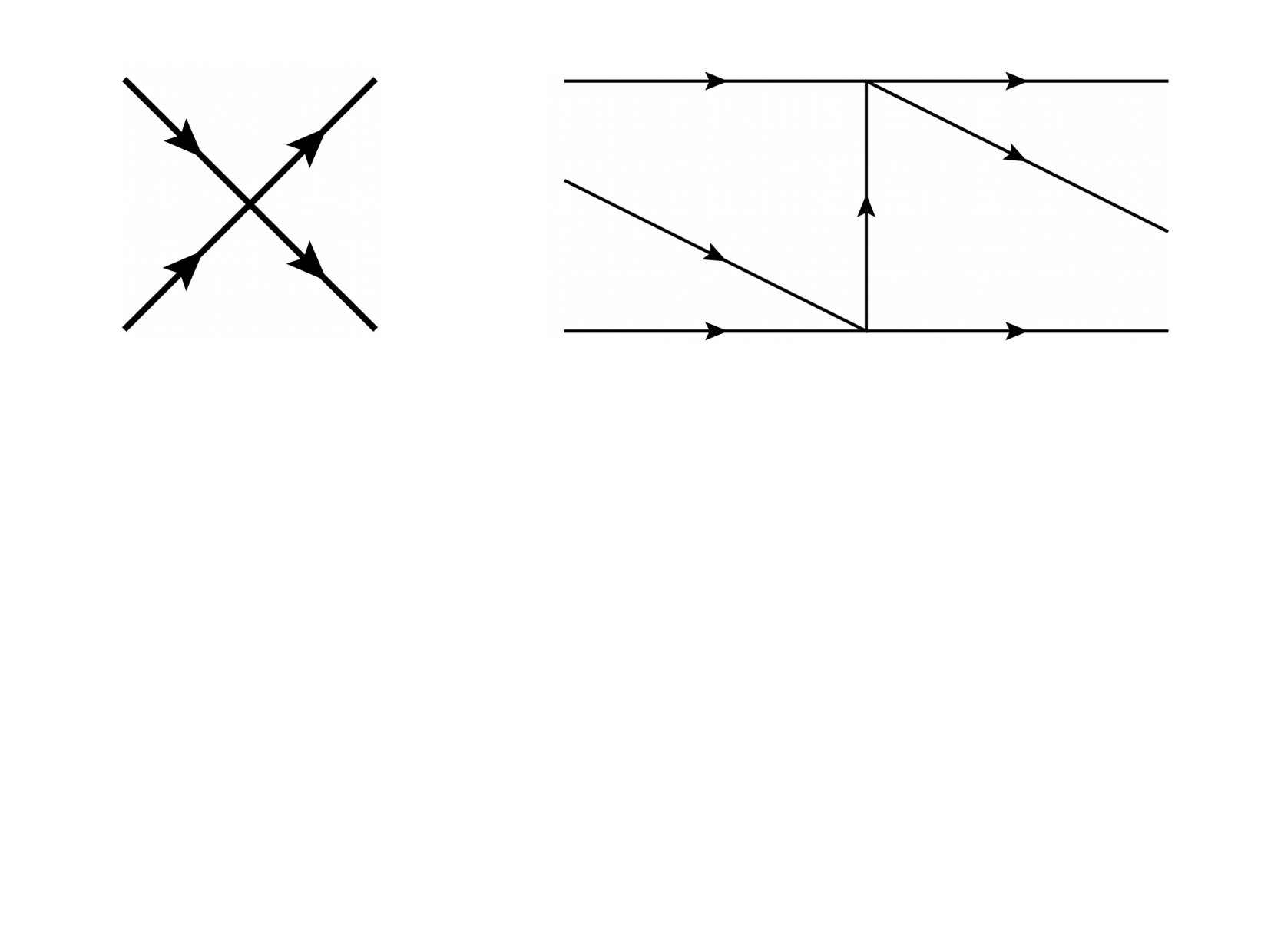 Figure 1
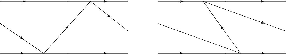 Figure 2
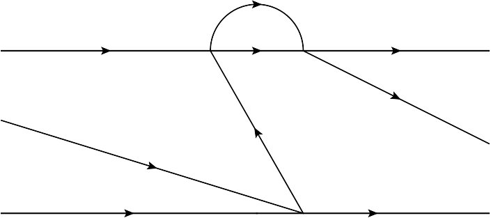 Figure 3
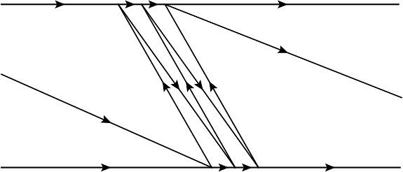 Figure 3
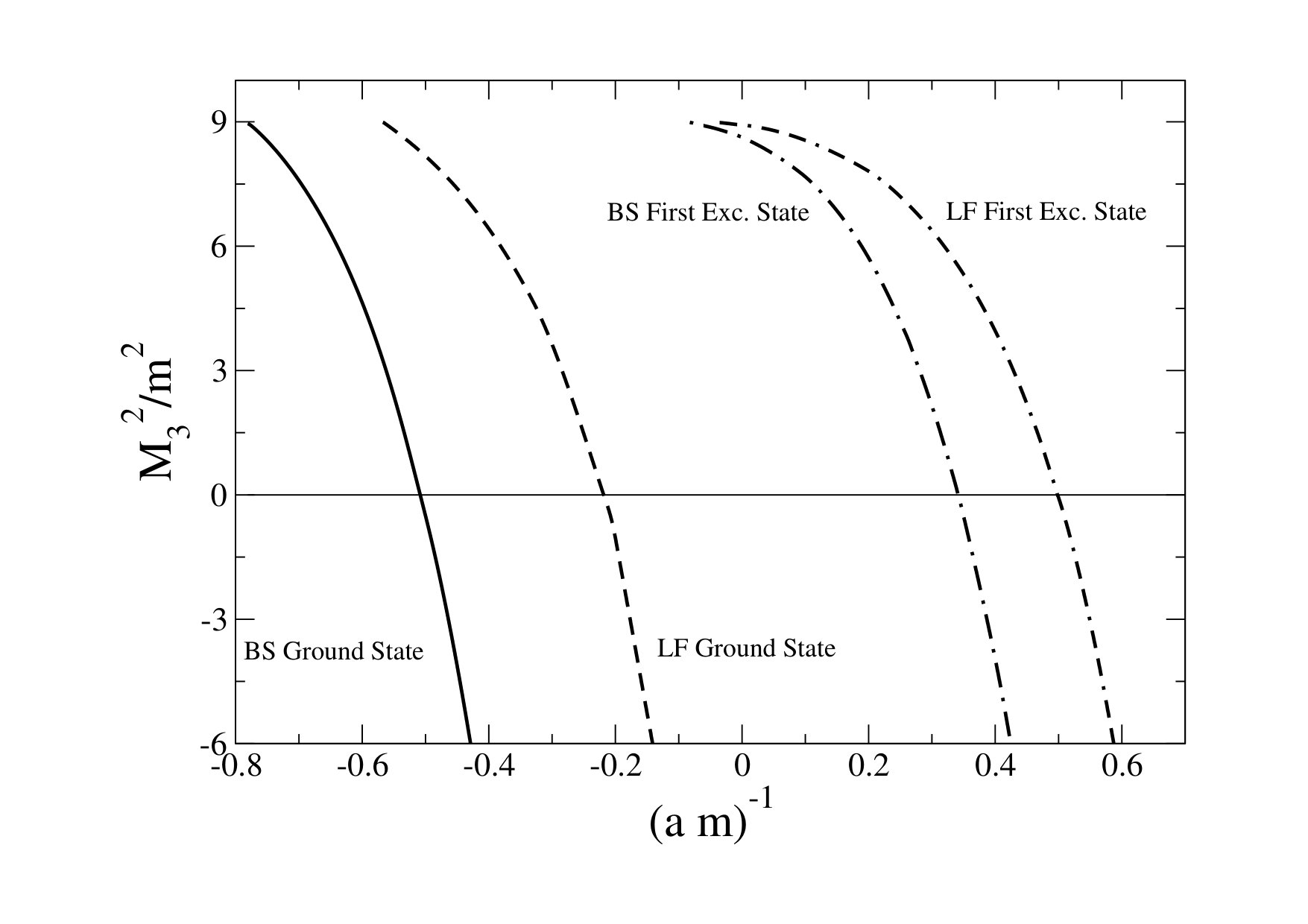 Figure 4
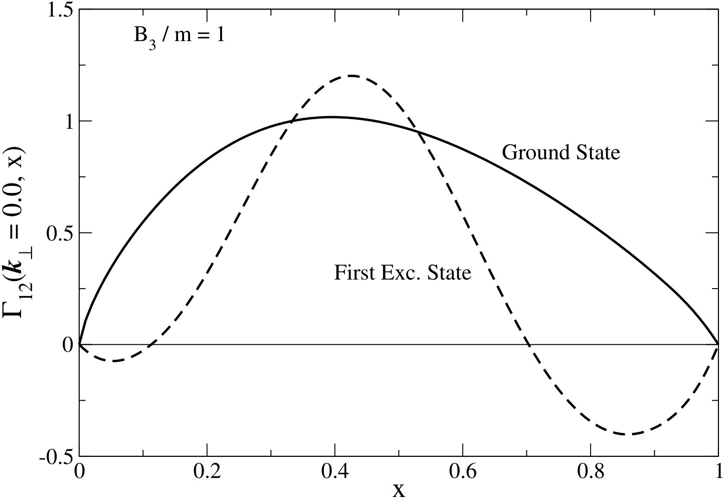 Figure 5
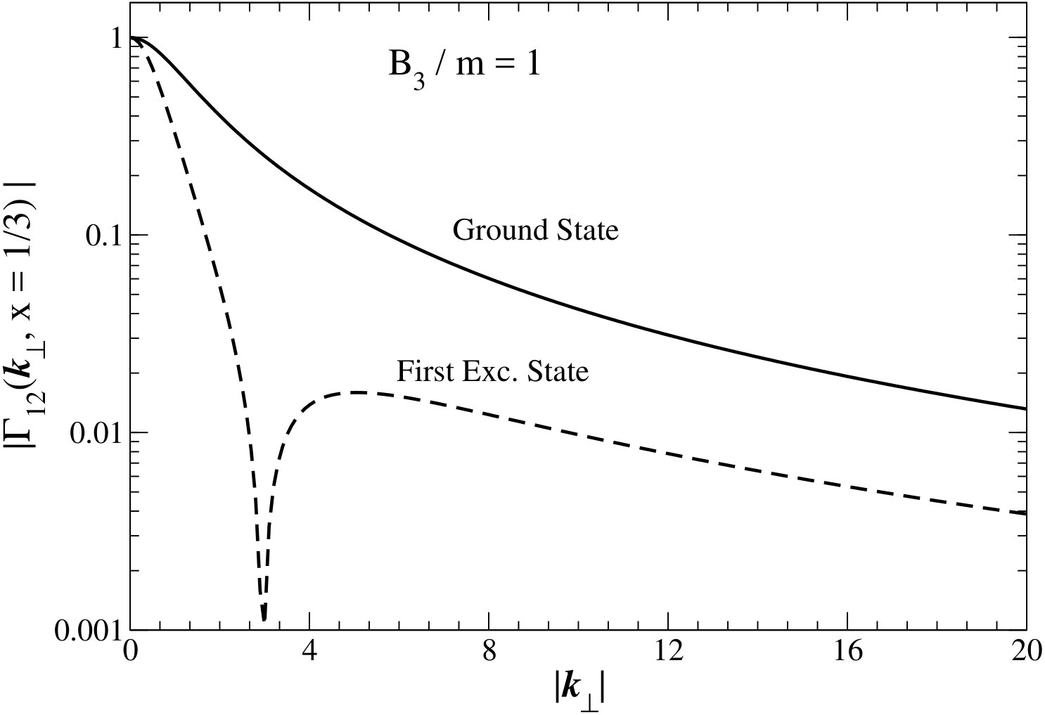 Figure 5
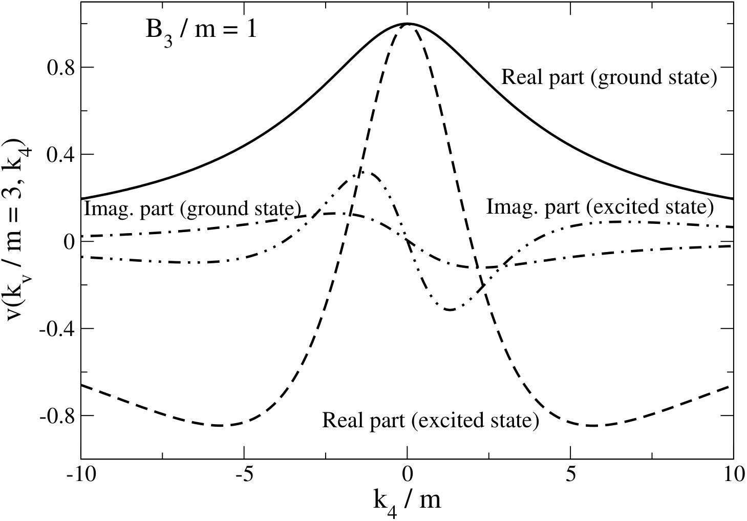 Figure 6
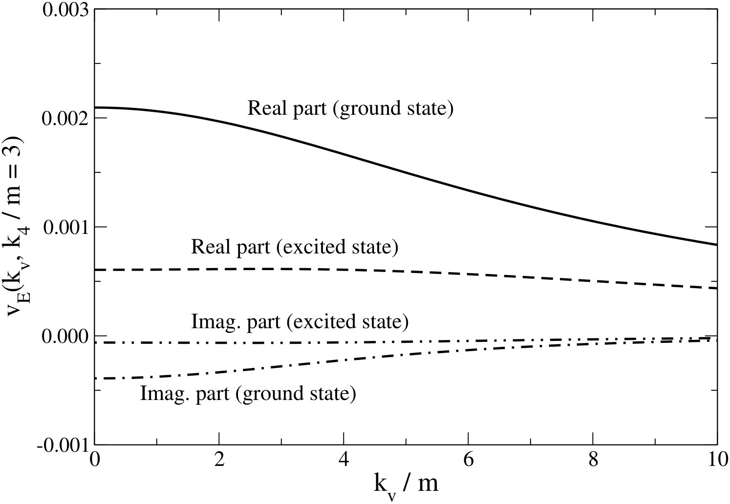 Figure 6
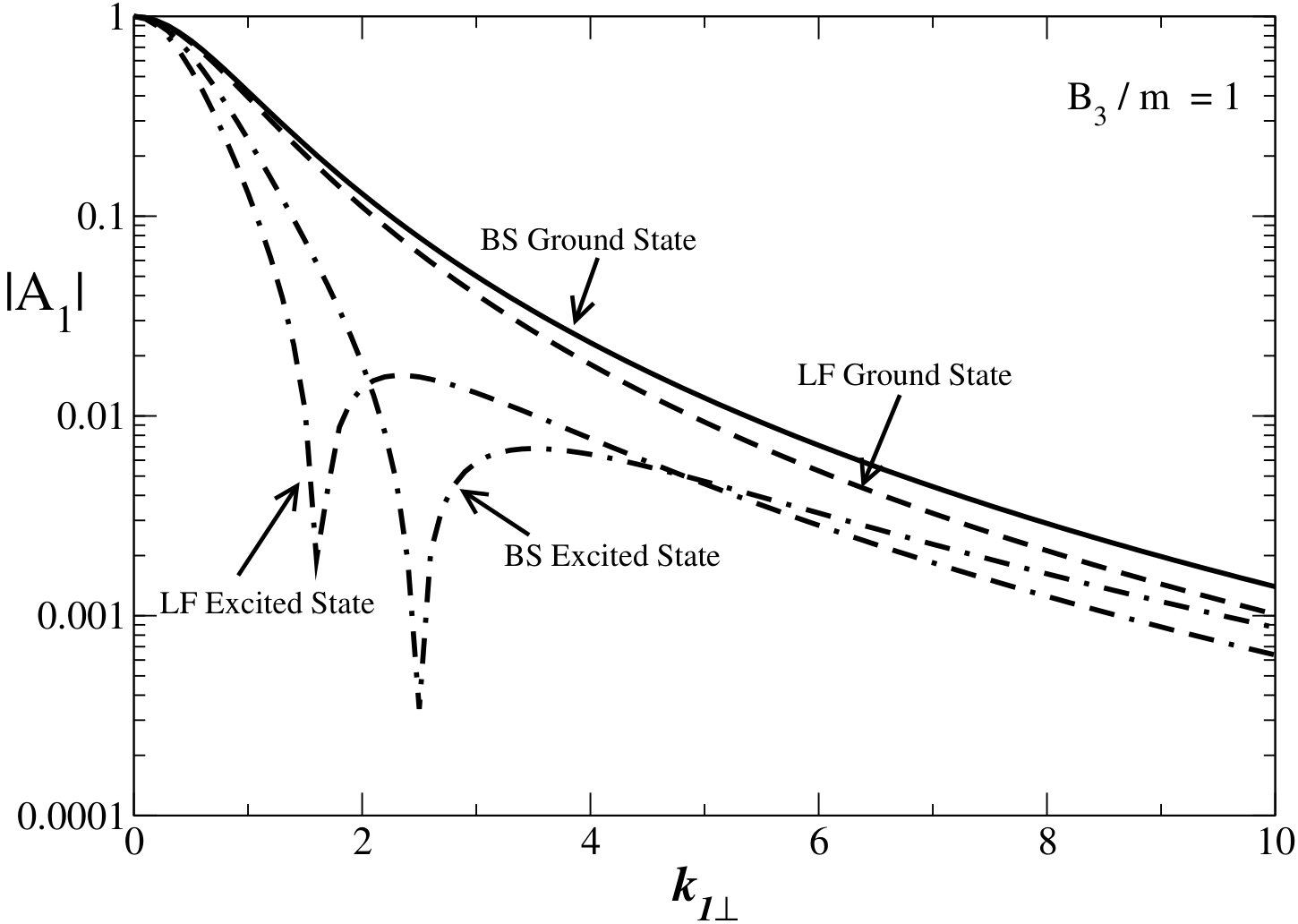 Figure 7
| Inverse scattering length | ||||
| ground state | excited state | |||
| BS | LF | BS | LF | |
Peer Reviews
No public reviews on file for this paper yet. If you reviewed it on a platform where reviews are public (OpenReview, ICLR, NeurIPS, ICML), you can paste yours below so the community can read it here.
Videos
No videos yet. Explain this paper in a talk, walkthrough, or lecture? Add one.
Three-body bound states with zero-range interaction in the Bethe-Salpeter
approach
E. Ydreforsa
J. H. Alvarenga Nogueiraa
V. Giganteb
T. Fredericoa
V.A. Karmanovc
aInstituto Tecnológico de Aeronáutica, DCTA, 12228-900 São José dos Campos, Brazil
bLaboratório de Física Teórica e Computacional - LFTC, Universidade Cruzeiro do Sul,
01506-000 São Paulo, Brazil
cLebedev Physical Institute, Leninsky Prospekt 53, 119991 Moscow, Russia
Abstract
The Bethe-Salpeter equation for three bosons with zero-range interaction is solved for the first time. For comparison the light-front equation is also solved. The input is the two-body scattering length and the outputs are the three-body binding energies, Bethe-Salpeter amplitudes and light-front wave functions. Three different regimes are analyzed: (i) For weak enough two-body interaction the three-body system is unbound. (ii) For stronger two-body interaction a three-body bound state appears. It provides an interesting example of a deeply bound Borromean system. (iii) For even stronger two-body interaction this state becomes unphysical with a negative mass squared. However, another physical (excited) state appears, found previously in light-front calculations. The Bethe-Salpeter approach implicitly incorporates three-body forces of relativistic origin, which are attractive and increase the binding energy.
keywords:
Bethe-Salpeter equation, light-front dynamics, zero-range interaction, relativistic three-body bound states.
††journal: Physics Letters B
1 Introduction
The zero-range interaction model is, undoubtedly, one of the oldest and most essential models in nuclear physics. It provides a reference framework and allows us to qualitatively grasp some important features of the nucleon-nucleon interaction. Understanding what happens in the limiting case of the zero-range interaction help us to clarify qualitatively the effect of a cutoff associated with a finite range interaction. That’s why it is useful to find and compare the solutions for the zero-range interaction for different few-body systems in various approaches. It is well known that in a non-relativistic three-body system with zero-range interaction the binding energy is not limited from below (Thomas collapse [1]). A variational proof of the Thomas effect in non-relativistic three-body systems can be found in [2] and the non-relativistic limit of few-body systems for the theory was studied in [3]. For the relativistic three-body bound system with zero-range interaction the covariant Bethe-Salpeter (BS) equation for the Faddeev component was derived in [4]. In that work, the corresponding three-body equation in the light-front (LF) dynamics was also derived by projecting the BS equation on the LF plane. Later it was re-derived independently of the BS approach, i.e., in the LF framework only [5]. In both papers [4, 5] the LF equation was solved numerically. In the aforementioned references it was concluded that the Thomas collapse is prevented in relativistic three-body systems, since the relativistic effects generates an effective repulsion at small distances.
The three-body BS equation with zero-range interaction was never solved so far. Finding its solution has remained for a long time an important and challenging problem. Of course, after avoiding the Thomas collapse in the LF framework, used in the previous works where only the valence component was considered, one can hardly expect that it will again appear in the BS framework. However, there are other important questions which can be clarified by solving the three-body BS equation and comparing the result with the LF one. For example, higher Fock components can have a significant effect even in two-body systems as shown in [6] and it is expected to be even more substantial in the three-body case [7].
The aim of this paper is thus two-fold:
(i) We solve, for the first time, the three-body BS equation with the zero-range interaction. For this aim, we transform the Minkowski BS equation in a suitable form to be expressed in the Euclidean space. From the point of view of time-ordered graphs appearing in LF dynamics, the three-body BS equation takes into account extra graphs incorporating antiparticles. In fact, they generate the effective three-body forces of relativistic origin. For the one boson exchange (OBE) interaction, the manifestation of the LF induced three-body forces was studied in [7]. In the OBE model the three-body forces appear also in absence of antiparticles whereas, as it is found in that paper, for the zero-range interaction, the intermediate antiparticles are mandatory for generating the three-body forces. Comparison of the results found by solving the LF and BS equations is instructive and it sheds light on the properties of the relativistic three-body systems with the zero-range interaction. We will calculate and compare also the dependencies of the LF and BS amplitudes on the transverse momenta. Fully Poincaré-covariant computation of the nucleon’s Faddeev amplitude with a ladder dressed-gluon exchange interaction was performed in [8] (see [9] for a review).
(ii) It turns out that though the three-body state studied in [4, 5] for the interaction providing the existence of a two-body bound state is indeed the most low-lying physical state (with minimal positive three-body mass ), there exists another (non-physical) low-lying state with negative . This is a “heavy legacy” of the Thomas collapse. Formally, from the point of view of the spectrum classification, the latter state is just the ground state (since it has the smallest ), whereas the state found in [4, 5] (and interpreted as the ground state) is the first excited state. By varying the two-body scattering length, we can push the ground state into the domain of the positive mass , so it becomes a physical state. In this situation the excited state found in [4, 5] does not exist anymore, since it was already driven into the continuous spectrum. This happens in both approaches – the LF and BS ones, and the difference between them is in the numerical values of the parameters, as we will show here. Below we will discover and study this true low-lying state. This is another aim of our work.
The rest of this paper is organized as follows. In Sections 2 and 3 we present the three-body BS and LF equations. In Sec. 4 is devoted to the derivation of the -dependent amplitudes in terms of the LF wave function and the BS Euclidean amplitude. In Sec. 5 we compute the positions of the ground and first excited levels and study how they move depending on variation of the two-body interaction. Sec. 6 presents the numerical results for the LF wave function, BS amplitude and corresponding -dependent amplitudes. Finally, in Sec. 7 we draw the conclusions.
2 Bethe-Salpeter equation
The zero-range three-body BS equation for the vertex function from which the external propagators are excluded, for zero-range interaction, has the form [4]:
[TABLE]
Here is the Faddeev component and, besides the total momentum , it depends on one four-momentum only. The function is the two-body zero-range scattering amplitude found in a relativistic framework. It is given in [4, 5]. For completeness we cite it here, however, using as a parameter, the scattering length :
[TABLE]
Its argument is two-body effective mass: and , . If the two-body system has a bound state with the mass , then is positive and it is related to the bound state mass as:
[TABLE]
If , the amplitude has no pole in the physical domain , that is, the two-body bound state is absent. However, as we will see below, the three-body system still can be bound as a Borromean state.
As mentioned, to simplify finding the solution of eq. (1), instead of the Minkowski space BS equation (1), we will solve the corresponding integral equation in the Euclidean space. It provides the same spectrum, but different amplitudes.
The Euclidean equation is obtained by the Wick rotation of the integration contour, when it is possible. In Eq. (1) it is impossible: one can easily check that the position of singularities in the variable of the integrand in (1) prevents from this rotation. That is, the rotating contour crosses the singularities of the integrand. This was the obstacle in finding solution of Eq. (1). However, the shift of the rotation point changes the relative position of the rotating contour and singularities and might allow to avoid their crossings. We notice that the Wick rotation becomes possible after the following shift of variables:
[TABLE]
After introducing new functions:
[TABLE]
the equation (1) obtains the form:
[TABLE]
where . In the three-particle rest frame, for example, the position of the pole (above the real axes) of the second propagator in (5) in the variable is in the point , where
[TABLE]
For the bound state , the value of is always negative: . We rotate the line of integration over by the angle and simultaneously replace . Then the pole and the contour move so that the pole never crosses the contour.
The amplitude has also a pole at , corresponding to the two-body bound state, if any. It generates two poles in vs. . One can easily check that if (this is the case, since the three-body binding energy per particle is larger that the two-body one), then these poles also do not prevent the Wick rotation. Therefore we can safely make the Wick rotation in Eq. (5), in contrast to the Eq. (1).
In the rest frame, after Wick rotation by the angle : , and after integrating in (5) over the angles between and , we obtain the equation:
[TABLE]
where (similarly for ),
[TABLE]
and . Namely Eq. (7) will be solved numerically below.
By performing the complex conjugation in (7) and (7) and changing , we find the same equation for . Hence, , or:
[TABLE]
3 Light-front equation
In the LF framework, the equation for the Faddeev component of the three-body vertex function reads [4, 5]:111Eq. (11) from [4] differs from (10) by the integration limits incorporating cutoffs which are absent in (10).
[TABLE]
where is the invariant mass squared of the intermediate three-body state:
[TABLE]
The two-body scattering amplitude is still given by Eq. (2), but its argument – two-body effective mass – is defined now as
[TABLE]
In general, the Faddeev component depends on all the variables constrained by the conservation laws: . Due to the zero-range interaction, depends on one pair of these variables only [4] which we denote and .
Though both Eqs. (1) and (10) correspond to the zero-range interaction, the underlying dynamics is not identical. It is instructive to discuss this difference. The cross graph shown in left panel of Fig. 1 is the elementary two-body Feynman graph – a “building block”, associated with the two-body interaction, from which, connected by the propagators, all the graphs contributing to Eq. (1) are constructed. The lowest order three-body Feynman graph, constructed from two of these two-body interaction “blocks”, is shown in the right panel of Fig. 1. The LF graphs are obtained from the Feynman ones by the time-ordering of all the vertices (omitting the graphs with creation from vacuum, when they appear). One Feynman graph in the right panel of Fig. 1 (contributing, as the second iteration, in the BS equation (2)) corresponds to two time-ordered graphs shown in Fig. 2. For the ladder kernel, only the first graph of Fig. 2 contributes in the LF equation (3). The graph shown in the right panel of Fig. 2 contains the five-body intermediate state (including one antiparticle), but not the three-body one. This irreducible graph contributes to the effective three-body forces of relativistic origin. The graphs of this type (or more complicated ones) do not appear within the LF graph technique when one iterates the graph shown in left panel of Fig. 2. This is just the main difference between Eqs. (1) and (10): Eq. (10) contains the three-body intermediate states only (like Fig. 2, left panel), whereas Eq. (1), from the point of view of LF dynamics, takes into account the graphs of the type shown in the right panel of Fig. 2, and also more complicated ones. Examples of more complicated LF graphs are shown in Fig. 3. They provide further contributions to the three-body forces of relativistic origin. They are not included in Eq. (3), in the ladder approximation. However, they implicitly are taken into account by the BS equation (2) and they appear explicitly after its LF projection. Thus, the graph shown in the right panel of Fig. 3 contains up to nine particles in the intermediate state. These examples show that the number of particles in the intermediate states is not restricted - it can be arbitrary. By comparing the results found by Eqs. (1) and (10), we study the influence on the binding energy coming from these graphs with the anti-particles in the intermediate states, which are generating the LF effective three-body forces. We emphasize that the graph shown in the right panel of Fig. 1 does not generate the three-body forces in the BS equation (1). The graphs shown in Fig. 2 (right panel) and Fig. 3 represent the three-body forces in the LF equation (10). Note also that this model does not correspond to the theory since all the graphs incorporated by the interaction in Eq. (1) is still a small part of the full set of possible contributions to the kernel in the theory.
4 Amplitudes depending on transverse momenta
In the BS amplitude, instead of one can introduce the LF variables , where . The LF wave function is related to the integral over of the Minkowski BS amplitude. There is no corresponding relation in the Euclidean space. However, since the double integrals of the Minkowski BS amplitude over and , and of the Euclidean one over are the same (up to a Jacobian), this allows us to relate the integral of the Euclidean BS amplitude with an integral of the LF wave function. The relation was found in [10] and used in [11] for two-body systems. Below we will derive this relation for the three-body case.
The full vertex function is given by the sum of the Faddeev components. Correspondingly, the wave function is obtained from the vertex one by dividing by the energy denominator:
[TABLE]
where is defined by (11).
For the BS amplitude, the energy denominator is replaced by the product of three propagators:
[TABLE]
where .
In the three-body case we start with a 4D integral (over and ) from the Euclidean BS amplitude. We can integrate analytically over two of the four variables, which do not enter in the argument of . Similarly, we obtain a 2D integral (over and ) from the LF wave function. We can integrate analytically over one of these variables. In this way, for the LF wave function contribution we find:
[TABLE]
where
[TABLE]
and
For the Euclidean BS contribution we get:
[TABLE]
[TABLE]
where and
[TABLE]
Analogous formulas are easily found for and .
If the LF wave function is obtained by the LF projection of the BS amplitude, then , Eq. (14), must coincide with , Eq. (15). If the LF wave function is found from Eq. (10) and the BS amplitude is found from Eq. (7), then and differ because of different input in the kernels of Eqs. (10) and (1). The comparison of with shows the influence of the many-body intermediate states on the -dependence of the amplitude .
5 The two lowest-lying levels
In this section we present the numerical results for the ground and first excited states. Both LF and BS equations are solved by means of spline decomposition and the results are presented within the convergence , which is enough for our purposes.
We expect that the spectra of both equations are rather rich. However, as we said, we restrict ourselves to two low-lying states. The LF equation (10) determines the value . The situation with the BS equation (7) is the same. At a first glance, the BS equation determines in the first degree. However, the change of the sign is equivalent to the complex conjugation, which does not change the real eigenvalues. Hence, Eq. (7) also determines . Though originally appears as squared, when this parameter is found from the equations, it can have any sign. The relativistic effects eliminate the Thomas collapse, i.e., they do not allow the eigenvalues to decrease down to , though they do not prevent the value of from being negative for strong enough two-body interaction. It turns out that “strong enough” is already the interaction forming a two-body state with the binding energy close to zero – it provides negative for the ground state. However, when we further weaken the two-body interaction (the scattering length becomes negative and then ), the ground state value of becomes positive and then (), i.e., the three-body bound states disappear. The plot of vs. the inverse scattering length is shown in Fig. 4. Note that in the previous papers [4, 5] just the “LF-excited state” was studied. Our present calculations confirm the values vs. found in [5].
Fig. 4 shows that the three-body mass found in the BS approach is always smaller than found in the LF one. This means that the three-body forces discussed in Sec. 3 are attractive and strong. This conclusion coincides with the result found in Refs. [12, 7] for the OBE kernel. The dimensionless values for which the values cross zero and cross (when the three-body binding energy crosses zero) are given in the Table 1. The positive inverse scattering lengths (BS) and (LF), for which for excited state crosses zero, correspond, according to Eq. (3), to the two-body binding energies and , respectively. When , the ground state values are for the BS equation and for the LF one. They are extremely over-bounded. The corresponding excited state values (when ) are for the BS equation and for the LF one. The latter value is close to one computed in [5].
6 Light-front vertex function and Bethe-Salpeter amplitude
In order to study how the binding energy impacts the behavior of the solution, we vary the two-body parameters to obtain, in the LF framework, the binding energy , first, for the ground state (in this case: ), then, for the excited state (in this case: ). These two solutions of the LF equation (10), corresponding to the same binding energy, but to different states (ground and excited ones) and normalized by , are compared in Fig. 5. Though, in general, they considerably differ from each other, the functions vs. for the ground and excited states have the same asymptotic decrease, though with different coefficients: for the excited state is ten times smaller than for the ground state.
The asymptotic behavior of follows from Eq. (10). Up to the logarithmic correction resulting from , the asymptotic -dependence is provided by the factor that gives , which is close to the asymptotic form of both curves shown in the right panel of Fig. 5. Whereas, in the the non-asymptotic domain and the factor are determined by the integral in l.h. side of Eq. (10) which is sensitive to the details of . Therefore they strongly depend on the state.
The solutions of the Euclidean BS equation (7) for [ for the ground state and for the excited state] are shown in Fig. 6. Note that vs. is symmetric relative to and is antisymmetric, in accordance with Eq. (9).
The comparison of the -dependences of the LF and BS amplitudes is shown in Fig. 7. Though the full amplitudes are given by sums of three Faddeev components (Eq. (14) in the LF approach and Eq. (15) in the BS approach), we present the contributions of one component only, i.e., , Eq. (14), in comparison to , Eq. (15), each of them depends on and . We put , normalize both to 1 at and compare their dependencies. The calculations were carried out for in both approaches. The node structure is clearly visible in the figure. This is important since the number of nodes is a way of characterizing states and the ground state has no node, while the first excited state presents one.
One can see in Fig.7 that for the same three-body binding energy, the BS approach results in a wider distribution than the LF one. This reflects the effect coming from the three-body graphs that are not considered in the LF truncated equation. If we compare the - dependences obtained from Minkowski and Euclidean BS equations we should obtain the same result, as shown in [11] for the two-body case. In any given approach (BS or LF), the large momentum behavior of the excited state is the same as for the ground one, though BS and LF asymptotics look slightly different from each other.
7 Conclusion
We have found the ground and first excited state solutions for the three-boson system with zero-range interaction in the framework of two relativistic approaches: Bethe-Salpeter equation in the Euclidean space and light-front dynamics. In the BS framework, the solution was found for the first time. Our input is the two-body scattering length (or binding energy), the output is the three-body binding energies, the light-front wave functions and Bethe-Salpeter amplitudes.
We confirmed the value of binding energy found previously [5] in the LF framework. In addition, we found that the calculations [4, 5] dealt with the first excited state, though for the two-body interaction which allows the two-body bound state (used in [4, 5]), there is a three-body ground state but with non-physical negative squared mass, . This solution formally exists, but not as a physical state. The negative (though finite) can be interpreted as collapse of a relativistic system. However, for a two-body interaction characterized by negative scattering length (i.e. no two-body bound state), the aforementioned three-body state becomes physical, i.e. having positive . We get a strongly bound Borromean system for the negative scattering length, that is rather curious. Another way to avoid the negative is to introduce a cutoff. We expect that a cutoff can also weaken the two-body interaction and make positive. By a further decrease of the two-body interaction the three-body binding energy tends to zero so that the three-boson system becomes unbound.
We have also found that in spite of the same zero-range interaction, the dynamical contents in both approaches – BS and LF – are different. Relative to the LF dynamics, the BS approach implicitly takes into account the antiparticles and the many-body intermediate states which generate the effective three-body forces of the relativistic origin, like it happens for the OBE kernel [7], but with smaller diversity of the graphs contributing to three-body forces. However, their net effects is the same - the increase of the effective attraction and, consequently, the binding energy in the BS framework with respect to the LF one. At the same time, the fully relativistic effects in both frameworks are the effective repulsion, eliminating the Thomas collapse [1] in a three-boson system. This was found earlier in the LF approach [4, 5]. In the present paper this is confirmed also in the BS approach.
A comparison of the LF wave function with the Euclidean BS amplitude cannot be done directly, since these quantities have different nature and physical meaning. However, as it is shown in Sec. 4, the integrals calculated from both quantities, either over , or over and , represent one and the same amplitude depending on transverse momenta (provided, the underlying dynamics is the same). At the same time, the contributions from three-body forces discussed in Sec. 3, that makes different the binding energies, also affects the -amplitudes. We compared these amplitudes for the same binding energy of the three-body system and we found that in the BS approach the -distributions are somewhat wider than in the LF one.
The solutions and observations found in this work deepen our understanding of the role of relativistic effects in three-body systems. This research can be generalized to systems with non-equal masses [13], which naturally may have a richer spectrum.
Aсknowledgements. We thank the support from Conselho Nacional de Desenvolvimento Científico e Tecnológico (CNPq) and Coordenação de Aperfeiçoamento de Pessoal de Nível Superior (CAPES) of Brazil. J.H.A.N. acknowledges the support of the grant #2014/19094-8 and V.A.K. of the grant #2015/22701-6 from Fundaçãode Amparo à Pesquisa do Estado de São Paulo (FAPESP). V.A.K. is also sincerely grateful to group of theoretical nuclear physics of ITA, São José dos Campos, Brazil, for kind hospitality during his visit.
The reference list from the paper itself. Each links out to its DOI / PubMed record.
- 1[1] L.H. Thomas, Phys. Rev. 47 (1935) 903.
- 2[2] F. A. B. Coutinho, J. F. Perez, W. F. Wreszinsk, J. Math. Phys. 36 (1995) 1625.
- 3[3] F. A. B. Coutinho, J. F. Perez, W. F. Wreszinsk, Ann. Phys. 277 (1999) 94.
- 4[4] T. Frederico, Phys. Lett. B 282 (1992) 409.
- 5[5] J. Carbonell, V.A. Karmanov, Phys. Rev. C 67 (2003) 037001.
- 6[6] V. Gigante, J.H. Alvarenga Nogueira, E. Ydrefors, C. Gutierrez, V.A. Karmanov and T. Frederico, Phys. Rev. D 95 (2017) 056012.
- 7[7] V.A. Karmanov and P. Maris, Few-Body Syst. 46 (2009) 95.
- 8[8] G. Eichmann, R. Alkofer, A. Krassnigg, and D. Nicmorus, Phys. Rev. Lett. 104 (2010) 201601.