Quantum Turing Machines Computations and Measurements
Stefano Guerrini, Simone Martini, Andrea Masini

TL;DR
This paper introduces a comprehensive definition of quantum Turing machines (QTMs) that incorporates infinite computations, superpositions, and limits, aiming to unify existing models and define a class of quantum computable functions.
Contribution
It extends and unifies previous QTM models by allowing arbitrary quantum inputs, superpositions, and infinite computations with limit-based outputs, and proposes a robust observation protocol.
Findings
Defined a new model of QTMs with infinite computations and superpositions.
Established a class of quantum computable functions mapping quantum states to probability distributions.
Proposed an observation protocol that preserves outcome probabilities.
Abstract
Contrary to the classical case, the relation between quantum programming languages and quantum Turing Machines (QTM) has not being fully investigated. In particular, there are features of QTMs that have not been exploited, a notable example being the intrinsic infinite nature of any quantum computation. In this paper we propose a definition of QTM, which extends and unifies the notions of Deutsch and Bernstein and Vazirani. In particular, we allow both arbitrary quantum input, and meaningful superpositions of computations, where some of them are "terminated" with an "output", while others are not. For some infinite computations an "output" is obtained as a limit of finite portions of the computation. We propose a natural and robust observation protocol for our QTMs, that does not modify the probability of the possible outcomes of the machines. Finally, we use QTMs to define a class of…
Click any figure to enlarge with its caption.
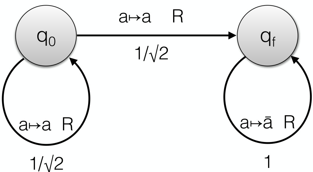 Figure 1
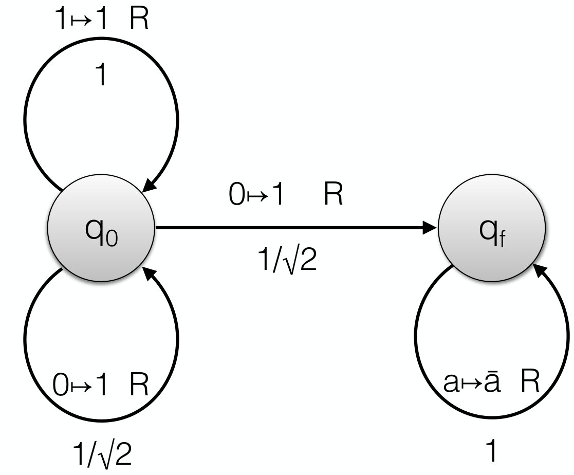 Figure 2
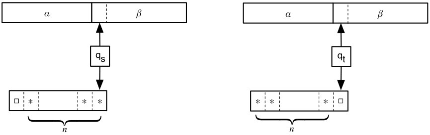 Figure 3
 Figure 4
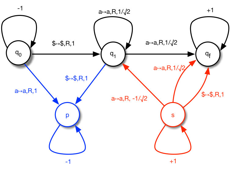 Figure 5
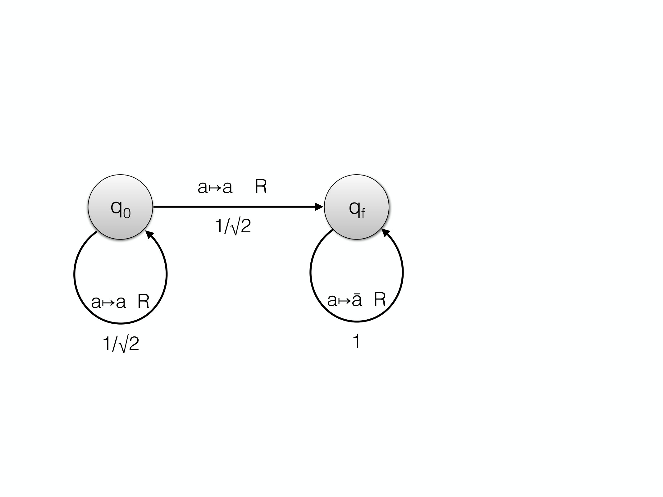 Figure 6
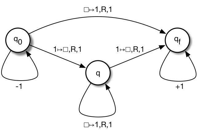 Figure 7
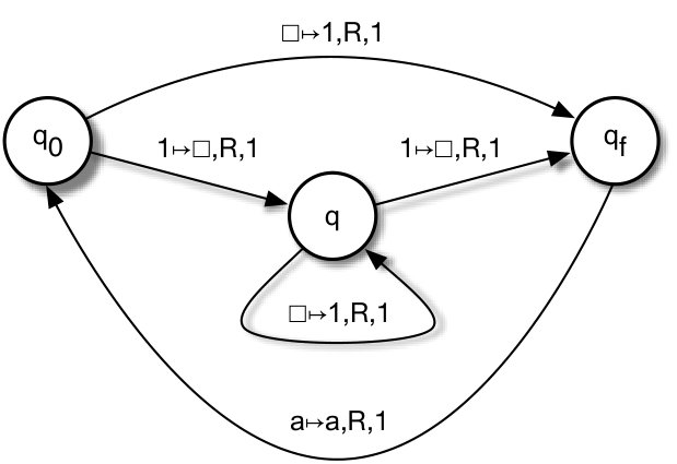 Figure 8
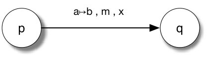 Figure 9
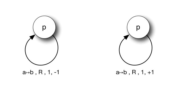 Figure 10
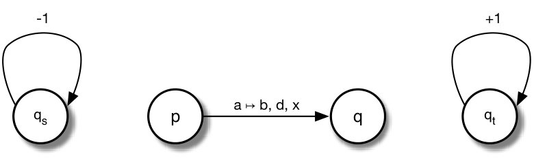 Figure 11
Peer Reviews
No public reviews on file for this paper yet. If you reviewed it on a platform where reviews are public (OpenReview, ICLR, NeurIPS, ICML), you can paste yours below so the community can read it here.
Videos
No videos yet. Explain this paper in a talk, walkthrough, or lecture? Add one.
Quantum Turing Machines:
computations and measurements
Stefano Guerrini
Stefano Guerrini
LIPN, UMR 7030 CNRS, Institut Galilée, Université Paris13, Sorbonne Paris Cité
,
Simone Martini*§*
Simone Martini
Dipartimento di Informatica – Scienza e Ingegneria, Università di Bologna, and Inria Sophia-Antipolis
and
Andrea Masini
Andrea Masini
Dipartimento di Informatica, Università di Verona
Abstract.
Contrary to the classical case, the relation between quantum programming languages and quantum Turing Machines (QTM) has not being fully investigated. In particular, there are features of QTMs that have not been exploited, a notable example being the intrinsic infinite nature of any quantum computation. In this paper we propose a definition of QTM, which extends and unifies the notions of Deutsch and Bernstein & Vazirani. In particular, we allow both arbitrary quantum input, and meaningful superpositions of computations, where some of them are “terminated” with an “output”, while others are not. For some infinite computations an “output” is obtained as a limit of finite portions of the computation. We propose a natural and robust observation protocol for our QTMs, that does not modify the probability of the possible outcomes of the machines. Finally, we use QTMs to define a class of quantum computable functions—any such function is a mapping from a general quantum state to a probability distribution of natural numbers. We expect that our class of functions, when restricted to classical input-output, will be not different from the set of the recursive functions.
Keywords: Quantum Turing Machines; Computability theory; Computer science; Theory of programming languages.
To appear on Applied Sciences, MDPI
§ Research partially conducted while on sabbatical leave at the Collegium – Lyon Institute for Advanced Studies, 2018-2019; partial support from INdAM-GNSAGA
1. Introduction
It is an early recognition of computer science that programming (and programming languages) could benefit from solid semantical foundations. At the end of the 50s of last century, both for clarity purposes and for the need of an entrance ticket into the “science club”, some prominent scientists started using mathematical techniques for the description of programming languages (e.g., Chomsky’s generative grammars, in the form of Backus-Naur Form [1]). Even more important is the proposal of general semantical models for the meaning of programs, represented at its best by McCarthy’s “mathematical theory of computation” [18], where a definition of the class of computable functions is presented as a general model for the semantics of (Algol) programs. The model is clearly idealised, in which it assumes that execution happens without physical limitations of space and time, in what will be, from that moment onwards, the standard model for programming languages, where one may assume Turing-completeness, despite each implementation being a finite state machine. The standard model builds on a long process during which Turing machines are viewed as idealised models of actual computers, and thus provide a basis for some theoretical investigation, among which the first studies on computational complexity.
Quantum computations and quantum programming languages have followed a different path. A solid and ever growing body of research is present on semantics and mathematical methods (e.g., see [8, 9, 34, 32, 27, 17, 26]) , but the relations of these languages with the basic notion of (quantum) Turing machines (as introduced by Deutsch in his seminal paper on quantum computation [11]; see also [2] for a quantum-mechanical model of Turing machines) has received much less study than in the classical case. The exception is, of course, the definition of quantum Turing machines (QTMs) by Bernstein & Vazirani [4] (B&V, from now on) and its use in the establishment of a sound quantum computational complexity. Their machines, however, have several strong constraints, reasonable for the purpose of a theory of computational complexity, but which do not permit to exploit all the features of the idealised model of computation that QTMs provide. In particular, meaningful computations are defined only for classical inputs (a single natural number with amplitude 1), and B&V’s “well-behaved” QTMs “terminate” synchronously—either all paths in superpositions enter a final state at the same time, or all of them diverge. As a consequence, there is no chance to study—and give meaning—to infinite computations, since for B&V’s “well-behaved” QTMs “non termination” corresponds to classical divergence.
Our aim is to provide a definition of QTMs with both quantum data and quantum control, hence broader than B&V’s one, and to base on this notion an explicit definition of a class of functions “computed by QTMs”. First of all, we allow a QTM to “start” its computation on an arbitrary quantum input—that is, a denumerable superposition of configurations, each representing a natural number. Second, since any computation of a QTM is always an infinite one, we want to give meaning also to some of these infinite computations. For such infinite behaviours, an “output” is obtained as a limit of finite portions of the computation. In order to accommodate these two aims with the unitary condition of the evolution, we have first to carefully define the very notion of QTM, in such a way that, when a computation of the machine enters into a “final state”, its evolution continues to remain in that final state, without changing the output written on the tape. This kind of evolution is obtained by enriching the machines by means of a suitable counter which plays no role during the standard evolution of the machine, but starts to be increased when a path of the computation enters into a final state. (A dual treatment, by reversibility, is done for the initial state.) Differently from B&V, any computation path (that is, any element of the superposition) evolves independently from the others: any path may terminate at its own time, or may diverge. Like B&V, we give local conditions ensuring that the resulting evolution respects the unitary condition.
We propose a suitable protocol for termination111In all the paper, with the exception of Section 6.2 when discussing papers of other authors, we use “termination” and not “halting.” Since there is no real halting for QTMs, we use a term different from the standard one used for classical TMs, to remark the difference. and observation of the result, which is robust with respect to the choice of the time instants in which the measurements for observing the results are made. This is in contrast to both B&V, where one has to know the exact termination time, and to Deutsch, where a partial measurement is made at every single step of the computation. The termination criteria for B&V and Deutsch is also one of the main obstacles for their use to define meaningful infinite computations.
Once we have a robust notion of QTMs and their observation protocol, we define the notion of “function computable by a QTM,” as a mapping between superpositions of initial classical configurations to probability distributions of natural numbers, which is obtained (in general) as a limit of an infinite QTM computation. Since not all infinite computations are meaningful to the limit, the resulting class of quantum computable functions contains also non-total functions, as it is usual in computability theory.
We stress that we are not proposing a kind of “super Turing computability”. We expect that our class of functions, when restricted to classical input-output and computable amplitudes, will be not different from the set of the recursive functions (see the end of Section 3.5).
We believe interesting to have a class of machines and functions which could be seen as a simple, and standard, model of quantum programs, thus opening the door to a quantum computability theory which could be of use for the semantics of quantum programming languages.
Organization of the paper
Section 2 introduces the central notion of Quantum Turing Machines; the technical definitions are preceded by a lengthy discussion on the motivations of the most delicate issues. We conclude the section with a theorem giving local conditions for unitarity, as in [4]. Section 3 uses QTMs to define a class of partial quantum computable functions. Section 4 deals with the problem of observables with respect to QTM computations. The protocols of Deutsch [11] and [4] are discussed, and a new observational protocol is proposed, proving that it agrees with the notion of computable functions of the previous section. In particular, we discuss in details Deutsch’s protocol, in which sense our proposal is different, and how it is related to Ozawa’s termination protocol [23]. In Section 5 we propose a detailed comparison with the approach of B&V. Section 6 is a detailed discussion of related work and other approaches. Finally, we discuss in the Appendix A some additional technical issues.
2. Quantum Turing Machines
In this section we define quantum Turing machines. Before the formal statements (Definitions 1, 6, 7, etc.) we will discuss in detail some of the notions that will be introduced, to motivate and explain our technical choices. We assume the reader be familiar with classical Turing machines (otherwise, see [10]), which we assume defined with a tape infinite in both directions.
Like a classical Turing Machine (TM), a Quantum Turing Machine (QTM) has a tape (a sequence of cells) containing symbols (one in each cell) from a finite tape alphabet , which includes at least the symbols and : is used to code natural numbers in unary notation, while is the blank symbol. We shall consider computations starting from tapes containing a sequence of symbols (the encoding of the natural number ); thus, in the following, for any , we shall use to denote the string . By the Greek letters , possibly indexed, we shall instead denote strings in , and by we shall denote the concatenation of and . Finally, we shall use to denote the empty string.
2.1. Plain configurations
The basic elements to describe the configuration of a QTM are the finite sequences of symbols on the tape (as usual, we assume that only a finite portion of the tape contains non-blank symbols), the current internal state of the machine, and the current position of the head reading a symbol in a cell of the tape. We assume that each cell of the tape has a fixed address (an integer number), corresponding to its position on the tape. That is, we assume the tape to be a function , such that, at any moment of the execution, only a finite, contiguous part of the tape is not empty, i.e., at any step of the execution, there are two constants s.t., for and (thus, when the tape is empty).
A canonical plain configuration of a given QTM is a quadruple , s.t.:
- (1)
is the current state, where is the finite set of the internal states of . 2. (2)
is the right content of the tape (w.r.t. the head position), where is the tape alphabet of the machine . If , the symbol is the current symbol, that is the content of the current cell, while is the longest string on the tape ending with a symbol different from and whose first symbol (if any) is written in the cell immediately to the right of the current cell. When instead, the right content of the tape, including the current cell, is empty, and the current symbol is . 3. (3)
is the left content of the tape (w.r.t. the head position). That is, it is either the empty string , or it is the longest string on the tape starting with a symbol different from , and whose last symbol is written in the cell immediately to the left of the current cell. 4. (4)
is the address of the current cell.
Given , let and , with . The plain configuration corresponds to the tape
[TABLE]
where , implies that .
In a canonical plain configuration the string does not start with a , and does not end with a . This ensures that each tape corresponds to a unique canonical plain configuration, and vice versa. However, since it will be useful to manipulate configurations which are extended with blank cells to the right (of the right content) or to the left (of the left content), we shall also consider plain configurations in which there is no restriction on and and we equate them up to the three equivalence relations induced by the following equations
[TABLE]
It is readily seen that any plain configuration is equivalent to a unique canonical plain configuration, and that two configurations are equivalent iff they are in the same state, the address of the head is the same, and they correspond to the same tape.
2.2. Hilbert space of configurations
We will see in the following that a quantum configuration of a QTM cannot be simply a plain configuration, but it must be a weighted superposition of configurations: a vector of the Hilbert space , where is a set of configurations, like the plain ones defined above.
We recall that, for any denumerable set , is the Hilbert space of square summable -indexed sequences of complex numbers
[TABLE]
equipped with an inner product and the euclidean norm , and that denotes the set of vectors .
By using Dirac notation, we shall write to denote the vector of corresponding to the function . Moreover, for every , we shall write to denote the vector corresponding to , that is, the function equal to on , and equal to [math] on the other elements of . Finally, we remark that any vector of can be written as , for some denumerable set of indexes s.t. and , for every . For more details on the basic notions of Hilbert spaces, see Appendix A.
2.3. Transitions of a QTM
Given a quantum configuration of a QTM (see Section 2.7 for the formal definition), the main idea introduced by Deutsch [11] is that the machine evolves into another quantum configuration , where is a unitary operator on the Hilbert space of the configurations of . By linearity and continuity, this also means that, if is the set of configurations on which we define the Hilbert space of quantum configuration of , the operator , and then the behaviour of , is completely determined by the value of on the elements of . B&V [4] refines this point by assuming that, as in a classical TM, for every , the transition from to a new configuration depends only on the current state of and on the current symbol of , and that is formed of configurations obtained by replacing the current symbol of with a new one, and by moving the tape head to the left or the right. Therefore, if we denote by the set of the possible movements on the tape (where stands for left and for right), and is the current state of , we have
[TABLE]
where ranges over the states of , ranges over its tape alphabet, , and is the new configuration obtained from by changing the current state from to , by replacing the current symbol with , and by moving the tape head in the direction .
2.4. Initial and final configurations
In B&V, the transition rule described above applies to every state of the machine. However, as already remarked in the introduction, this implies a severe restriction on the machines that one can actually consider as valid ones—the reversibility of unitary operators, and the problem of how to read the output, force to ask that, in a “well-behaved” QTM, if a configuration in superposition enters the final state, then all other configurations of the superposition must also enter into the final state.
The key point is that a QTM cannot stop into some final configuration , since the unitarity of requires that be defined. On the other hand, we cannot assume that, after reaching some final configuration , the computation loops on it neither. As this would imply that could not be reached from any other configuration : if , then , and , for . When a final configuration is reached, the machine must evolve into a different configuration which preserves the output written on the tape, without breaking the unitarity of the evolution operator . Let assume to have a denumerable set of indexed configurations obtained by adding a counter to , for every final configuration . The configuration plays the usual role of the plain configuration and it is the only one that can be reached from a non final configuration; for every , the configuration is instead the only successor of , that is, , where is the base vector corresponding to . In other words, the counter is initialised to [math] and plays no role while the state is not final; when a branch of the computation enters a final state, the counter is still at [math], but it is increased by at each following step.
Final configurations are not the only configurations on which it would be useful to loop. In some cases, in order to assure that the operator is unitary, we need to introduce additional target configurations that behave as sinks, from which the machine cannot get out (see Remark 2, and the example in Subsection 5.3, whose graph representation is given in Figure 4). We have then to consider a whole set of target states, containing the final state , s.t. for every plain configuration , with , we have a set of indexed configurations , for , s.t. .
Moreover, when is unitary, its inverse is unitary too, and can be applied to any initial configuration. Therefore, even if we assume that a computation always starts from some initial plain configuration , such a must have a predecessor , and more generally a -predecessor . As already done for final configurations, we associate to every a set of indexed configurations , with , s.t. , for . For , we get then ; while has the usual behaviour expected from the machine on the plain initial configuration . As for final state and final configurations, it is useful to generalise the above behaviour to a set of source configurations corresponding to a set of source states which contains the initial state .
2.5. Pre Quantum Turing Machines
In order to formally define QTMs, we first define a notion of pre Quantum Turing Machine, or pQTM. As we shall see later (Definition 10), a QTM is a pQTM whose evolution operator is unitary. Since the behaviour on target states and on source states whose counter is greater than [math] is fixed, in order to completely describe a pQTM, it suffices to give a transition function which, for every configuration with current state and current symbol , gives the weight of in the superposed configuration reached from , where is obtained by replacing for , by moving the tape in the direction, and by changing the current state to .
Definition 1** (Pre Quantum Turing Machine).**
Given a finite set of states and an alphabet , a pre Quantum Turing Machine (pQTM) is a tuple
[TABLE]
where
- •
* is the set of source states of , and is a distinguished source state named the initial state of ;*
- •
* is the set of target states of , and is a distinguished target state named the final state of ;*
- •
* and have the same cardinality and ;*
- •
* is the quantum transition function of , where .*
Remark 2** (Source and target states).**
Source and target states must be introduced to complete a QTM when the transitions implementing its expected behaviour fail to assure the local conditions of Theorem 15, required to get a unitary time evolution operator. In particular, the first condition states that the norm of the vector corresponding to the transition from a configuration with current state and current symbol , to a superposed configuration must be equal to 1. Anyhow, in some case, the norm of the vector of the weights implementing the expected behavior of the machine might give a value smaller than 1, while in no case it cannot exceed the value of 1. To achieve the required local condition, we can add some new transitions to some special target state acting as a sink (i.e., from which the machine cannot get out), with a procedure reminding the one used to complete a non-deterministic automata by connecting all the omitted transitions to a sink state. The main difference is that in the QTM case more than one target state may be necessary to achieve the goal. Moreover, because of the reversibility of QTMs, a similar condition must hold for the transitions entering into a given state. So, we must also take into account the case in which we need to complete the implementation of the expected behaviour by adding new transitions from some source states. Finally, we remark that the requirement that the sets of source and target states have the same cardinality is used to prove the unitarity of the evolution operator associated to our QTMs via a reduction to the B&V QTMs (see Theorem 15). We do have another, independent, and direct proof of this result (that we omit in this paper), and which also exploits the equinumerosity of source and target states. We conjecture then that this is indeed a necessary condition.
Remark 3** (On gödelization of QTMs).**
For a definition of gödelizable QTMs, we must restrict the definition of the transition function to computable complex numbers (see also [4].)
Definition 4** (computable numbers).**
*A real number is computable if there exists a deterministic Turing machine that on input computes a binary representation of an integer such that .
The set of the computable complex numbers is the set of the complex numbers whose real and imaginary parts are both computable.*
Now, let be the subset of s.t. the coefficients of the vectors are bound to be in . We can say that a transition function is computable when
[TABLE]
The gödelization of a QTM whose transition function is computable proceeds in the usual way. First of all, just observe that is a finite dimensional space, then that each complex number involved in the gödelization of can be replaced by a pair , where and are the Gödel numbers of the Turing machines computing and , respectively.
2.6. Configurations
We have already seen that, in order to properly deal with source and target states, we have to associate a counter to those states. For the sake of uniformity, we shall add a counter to every plain configuration. The counter will always be [math] for every non-source or non-target configuration.
Remark 5** (The counter).**
The counter can be seen as an additional device (for instance, as an additional tape or as a counting register) or directly implemented by a suitable extension of the basic Turing machine (for instance, by extending the tape alphabet). None of these implementations is canonical or has a direct influence in what will be presented in the following. A more detailed discussion of the implementation of the counter is given in Appendix B.
Definition 6** (configurations).**
Let be a pQTM. A configuration of is a quintuple , where is a plain configuration, and is a counter associated to the configuration s.t. , when . A configuration of is a source/target configuration when the corresponding state is a source/target state, and it is a final/initial configuration when the current state is final/initial. We have the following notations:
- •
* is the set of the configurations of .*
- •
* and are the sets of the source and of the target configurations of , respectively.*
- •
* and are the sets of the initial and final configurations of , respectively.*
- •
* is the set of the configurations of .*
In the following, the subscript in and in the other names indexed by the machine may be dropped when clear from the context.
2.7. Quantum configurations
The evolution of a pQTM is described by superpositions of configurations in . If is a set of configurations, a superposition of configurations in is a vector of the Hilbert space (see, e.g., [5, 29]). Quantum configurations of a pQTM are the elements of (namely, the unit vectors of ). Since there is no bound on the size of the tape in a configuration, the set is infinite and the Hilbert space of the configurations is infinite dimensional.
Definition 7** (quantum configurations).**
Let be a pQTM. The elements of are the quantum configurations (or more succinctly, q-configurations) of .
We shall use Dirac notation (see Appendix A) for the elements of , writing them .
Definition 8** (computational basis).**
For any set of configurations and any , let be the function
[TABLE]
The set of all such functions is a Hilbert basis for (see, e.g., [21]). In particular, following the literature on quantum computing, is called the computational basis of . Each element of the computational basis is called base q-configuration.
With a little abuse of language, we shall write when . The span of , denoted by , is the set of the finite linear combinations with complex coefficients of elements of ; is a vector space, but not a Hilbert space. In order to get a Hilbert space from we have to complete it, and is indeed the unique (up to isomorphism) completion of (see [4]). As a consequence, any bounded linear operator on has a unique extension on , and, when is unitary, its extension is unitary too.
For some basic definitions, properties and notations on Hilbert spaces with denumerable basis, see Appendix A. In particular, subsection A.1 presents a synoptic table of the so-called Dirac notation that we shall use in the paper.
2.8. Time evolution operator and QTM
In order to define the evolution operator of a pQTM , it suffices to give its behaviour on the computational basis . In particular, we have to distinguish three cases:
- (1)
.
Let be the configuration obtained by leaving the counter to [math], by replacing the symbol in the current cell with the symbol , by moving the head on the direction, and by setting the machine into the new state . In detail, if
we have
[TABLE]
and we define
[TABLE]
where is the quantum transition function of , and, as already introduced at the end of Section 2.3, is is the new configuration obtained from by changing the current state from to , by replacing the current symbol with , and by moving the tape head in the direction . 2. (2)
.
Let be the source configuration obtained by decreasing by the counter of , we define
[TABLE] 3. (3)
.
Let be the target configuration obtained by increasing by the counter of , we define
[TABLE]
We have then three linear operators
[TABLE]
defined on three disjoint subspaces. Moreover, since even the images of these three operators are disjoint, their sum
[TABLE]
defines an automorphism on the linear space of q-configurations
[TABLE]
Indeed, since is bounded, it extends in a unique way to a continuous operator on the Hilbert space of q-configurations.
Definition 9** (time evolution operator).**
The time evolution operator of is the unique continuous extension
[TABLE]
of the bounded linear operator .
As it is the case for the operator , also the time evolution operator can be decomposed into three operators
[TABLE]
s.t.
[TABLE]
Definition 10** (QTM).**
A pQTM is a Quantum Turing Machine (QTM) when its time evolution operator is unitary.
As usual, (the -th iterate of ) is defined as , and .
2.9. Computations
A computation of a QTM is an iteration of its evolution operator on some q-configuration. Since the time evolution operator of a QTM is unitary, it preserves the norm of its argument and maps q-configurations into q-configurations. By the way, this holds for the inverse of the time evolution operator, too.
Property 11**.**
Let be a QTM. If , then , for every .
Definition 12** (initial and final configurations).**
A q-configuration is initial when and is final when . By we denote the initial configuration .
Definition 13** (computations).**
Let be a QTM and let be its time evolution operator. For an initial q-configuration , the computation of on is the denumerable sequence s.t.
- (1)
; 2. (2)
.
Clearly, any computation of a QTM is uniquely determined by its initial q-configuration. The computation of on the initial q-configuration will be denoted by .
Remark 14**.**
The definition of the time evolution operator ensures that the final configurations reached along a computation are stable and do not interfere with other branches of the computation in superposition, which may enter into a final configuration later. Indeed, given a configuration , where and does not contain any final configuration, let . Any final configuration in has a value of the counter less than , while any final configuration formed of a plain configuration and a counter is mapped into a configuration . Moreover, and have the same coefficient in and , respectively, since .
2.10. Local conditions for unitary evolution
In analogy to the main approaches in the literature [4, 25], it is possible to state a set of local condition for the quantum transition function of pQTMs in order to ensure that the time evolution operator is unitary.
Theorem 15**.**
Let be a pQTM with quantum transition function . The time evolution operator of is unitary iff satisfies the local conditions:
- (1)
for any
[TABLE] 2. (2)
for any with
[TABLE] 3. (3)
for any
[TABLE]
where denote the complex conjugate operator.
Proof.
We show that, to any QTM (as defined above), we can associate a B&V QTM which differs on the behaviour on source and target states only. The unitarity of follows then from the unitarity of .
Let . We take the B&V QTM with the same states and the same alphabet , and whose transition function satisfies the following conditions:
- (1)
is the same of the transition function of for any non-terminal state; 2. (2)
for any terminal state and every current symbol , has a unique non-null transition, with weight , that leaves the current symbol on the tape unchanged, moves the head to the right, and goes into an initial state ; 3. (3)
the non-null out transitions from two distinct terminal states lead to two distinct source states, defining in this way a bijection between the set of the target and source states.
In other words, is defined by:
[TABLE]
The above definition ensures that is a B&V QTM whose configurations are the plain configurations of , and s.t. its transition function verifies B&V local conditions. By B&V, the evolution operator of is then a unitary operator on the Hilbert space of the plain configurations of and, as a consequence, its adjoint is its inverse. We can take three linear operators
[TABLE]
defined by
[TABLE]
Which are the inverses of the three corresponding linear operators , , and , respectively (see subsection 2.8). Thus, the bounded linear operator is the inverse of , and its continuous extension (obtained by completion) is the inverse of . Moreover, such an operator is the adjoint of also. Summing up, the adjoint of is its inverse and, as a consequence, is unitary. ∎
Remark 16**.**
The reader may wonder why we need to have cell indexes in configurations, when they are not used in many definitions of classical TMs. In fact, cell indexes are needed only in a very special case, that of a completely empty tape. Let us suppose, indeed, to eliminate indexes, and to feed a completely blank tape to a QTM with only two states , with no source and final states and no tape symbols except ; let the transition function be s.t.
- •
**
- •
**
- •
**
- •
**
- •
**
- •
**
- •
**
- •
**
It is easy to check that the conditions of Theorem 15 are satisfied, but trivially the induced time evolution operator is not an isometry since, given the empty string we have .222We omit here the counter, which always remains set to zero. The indexing we use is consistent with the one adopted by Bernstein & Vazirani, [4]–Definition 3.2, pag. 1419. Here we just want to point out that Bernstein & Vazirani only provides a fairly light informal definition of configuration. We have preferred a more pedantic formulation, which in our opinion is necessary to eliminate all the reader’s doubts about the correctness of the proposed theorems.
2.11. A comparison with Bernstein and Vazirani’s QTMs: part 1
We refer to B&V [4] for the precise definitions of the QTMs used in that paper. For the sake of readability, we informally recall the notion of what they call well formed, stationary, normal form QTMs (B&V-QTMs in the following).
A B&V-QTM is defined as our QTM (with one source state and one target state only) with the following differences:
- (1)
the set of configurations coincides with all possible classical configurations, namely all the set ; 2. (2)
no superposition is allowed in the initial q-configuration (it must be a classical configuration with amplitude 1); 3. (3)
given an initial configuration , the q-configuration is the final q-configuration for the computation starting in , when: (i) all the configurations in are final; (ii) for all , the q-configuration does not contain any final configuration. When this is the case, we also say that the QTM halts in steps in ; 4. (4)
if a QTM halts, then the tape head is on the start cell of the initial configuration; 5. (5)
there is no counter and for every symbol there is loop from the only final state into the only initial state , that is, for every . Therefore, because of the local unitary conditions (that must hold in the final state too), these are the only outgoing transitions from , and the only incoming ones into . So, if and if .
Theorem 17**.**
For any B&V-QTM there is a QTM s.t. for each initial configuration , if with input halts in steps in a final configuration , then .
Proof.
The QTM has the same states of , the initial state is its only source state, and the final state is its only target state. Therefore, if , we take , where is the restriction of to , that is, for each and , we have , for every . Since the local unitary conditions hold for and, in a B&V-QTM, , when , the unitary local conditions hold for too.
By construction, if is not final for , then . In particular, this holds when is the final configuration of the B&V-QTM . ∎
We remark that the inverse cannot hold true: A B&V-QTM for a given input cannot exhibit both a non terminated computation and a terminated one (see Example 5.3 for a machine that cannot be simulated by a B&V-QTM).
3. Quantum Computable Functions
In this section we address the problem of defining the concept of quantum computable function in an “ideal” way, without taking into account any measurement protocol. The problem of the observation protocol will be addressed in Section 4. Here we show how each QTM naturally defines a computable function from the sphere of radius in to the set of (partial) probability distributions on the set of natural numbers.
3.1. Probability distributions
Definition 18** (Probability distributions).**
**
- (1)
A partial probability distribution (PPD) of natural numbers is a function such that . 2. (2)
If , is a probability distribution (PD). 3. (3)
* and denote the sets of all the PPDs and PDs, respectively.* 4. (4)
If the set is finite, is finite. 5. (5)
Let be two PPDs, we say that () iff for each , (). 6. (6)
Let be a denumerable sequence of PPDs; is monotone iff , for each .
Remark 19**.**
*In the following, we shall also use the notation . By definition, , and a PPD is a PD iff . We also stress that is a partial order of PPDs and that any PD is maximal w.r.t. to . *
Definition 20** (limit of a sequence of PPDs).**
Let be a sequence of PPDs. If for each there exists , we say that , with .
3.2. Monotone sequences of probability distributions
Proposition 21**.**
Let be a monotone sequence of PPDs.
- (1)
* exists and it is the supremum of ;* 2. (2)
; 3. (3)
.
Proof.
Since , every non-decreasing sequence has a supremum . Thus, is defined and , for every . On the other hand, for any s.t. for , we have , for every ; namely, . We can then conclude (item 1) that .
Let us now prove item 2. First of all, since for , we have and
[TABLE]
for any . Thus,
[TABLE]
Summing up, we can conclude, as
[TABLE]
Finally, by hypothesis, , for any . Therefore, . Which proves (item 3) that . ∎
3.3. PPD sequence of a computation
The computed output of a QTM will be defined (Definition 26) as the limit of the sequence of PPDs obtained along its computations.
Definition 22** (probability and q-configurations).**
Given a configuration , let be the number of s in . For any , let us define s.t.
[TABLE]
when .
Proposition 23**.**
If is a q-configuration, is a PPD. Moreover, it is a PD iff is final.
Proof.
Let with , and . By the definition of , it is readily seen that and that . Therefore, is a PPD. Moreover, since iff . We see that is a PD iff , that is, iff . ∎
Definition 24**.**
For any q-configuration , we shall say that is the PPD associated to , and we shall denote by the sequence of PPDs associated to the computation .
The PPD sequence of any QTM computation is monotone. In the simple proof of this key property (Theorem 25) we see at work all the constraints on the time evolution of a QTM .
- (1)
That when in a final (target) configuration, the machine can only increment the counter; as a consequence, the of final (target) configurations does not change. 2. (2)
That when entering for the first time into a final (target) state, the value of the counter is initialised to [math]. 3. (3)
That when in a final (target) configuration , the counter gives the number of steps since is looping into the plain configuration .
We stress that the last two properties defuse quantum interference between final configurations reached in a different number of steps.
Theorem 25** (monotonicity of computations).**
For any computation of a QTM , the sequence of PPDs is monotone.
Proof.
Let us prove that , for every . Let , with , and , where is the set of the configurations of whose counter is equal to . For every , we see that . Let . By the definition of , we see that and . Therefore, .
∎
3.4. Computed output
We can now come back to the definition of the computed output of a QTM computation. The easy case is when a computation reaches a final q-configuration (meaning that all the classical computations in superposition are “terminated”)—in this case the computed output is the PD . The QTM keeps computing and transforming into other configurations, but all these configurations have the same PD. However, we want to give meaning also to “infinite” computations, which never reach a final q-configuration, yet producing some final configurations in the superpositions. For this purpose, we define the computed output as the limit of the PPDs yielded by the computation.
Definition 26** (computed output of a QTM).**
*Let be the computation of the QTM on the initial q-configuration . The computed output of on the initial q-configuration is the PPD , which we shall also denote by , or by the notation . *
Let us remark that, by Proposition 21 and Theorem 25, the limit in the above definition is well-defined for any computation. Therefore, a QTM has a computed output for any initial q-configuration .
Definition 27** (finitary computations).**
Given a QTM , a q-configuration is finite if it is an element of . A computation is finitary with computed output if there exists a s.t. is final and .
Proposition 28**.**
Let be a finitary computation with computed output , that is, .
- (1)
There exists a , such that for each , is final and . 2. (2)
* is a PD.*
Proof.
By definition, there is a s.t. is final. Let . By Proposition 23, is a PD. By monotonicity, , for every . Thus, since any PD is maximal for (see Remark 19), , for every . ∎
Given a computation , we can then distinguish the following cases:
- (1)
is finitary. In this case ; the output of the computation is then a PD and is determined after a finite number of steps; 2. (2)
is not finitary, but . The output is a PD and is determined as a limit; 3. (3)
is not finitary, and (the sum of the probabilities of observing natural numbers is ). Not only the result is determined as a limit, but we cannot extract a PD from the output.
The first two cases above give rise to what Definition 29 calls a q-total function. Observe, however, that for an external observer, cases (2) and (3) are in general indistinguishable, since at any finite stage of the computation we may observe only a finite part of the computed output.
For some examples of QTMs and their computed output, see Section 5.
3.5. Quantum partial computable functions
We want our quantum computable functions to be defined over a natural extension of the natural numbers. When using a QTM for computing a function, we stipulate that initial q-configurations are superpositions of initial classical (plain) configurations , where the tape of the configuration encodes the number . A natural choice for this encoding corresponds to take , where denotes the string . Such q-configurations are naturally isomorphic to the space of square summable, denumerable sequences with unitary norm, under the bijective mapping . Observe that, for output, we simply count the number of (non contiguous) s on the tape, according to Definition 22.
Definition 29** (partial quantum computable functions).**
**
- (1)
A function is partial quantum computable (q-computable) if there exists a QTM s.t. iff . 2. (2)
A q-partial computable function is quantum total (q-total) if for each , .
It is out of the scope of the paper to investigate in details how this class exactly relates to other classes of computable functions when the input of QTMs is restricted to classical inputs. Observe, however, that when also the output is required to be classical, and all amplitudes are computable, we expect to obtain the classical (partial) recursive functions. Indeed, any classical deterministic TM may be simulated by a reversible TM [3]; moreover, B&V show that reversible TMs are a special case of QTMs (their Section 4; see also our Section 5.2.). On the other direction, when we have classical inputs and computable amplitudes, it is easy to simulate a QTM via a classical TM.
4. Observables
While the evolution of a closed quantum system (e.g., a QTM) is reversible and deterministic once its evolution operator is known, a (global) measurement of a q-configuration is an irreversible process, which causes the collapse of the quantum state to a new state. Technically, a measurement corresponds to a projection on a subspace of the Hilbert space of quantum states. For the sake of simplicity, in the case of QTMs, let us restrict to measurements observing if a configuration belongs to the subspace described by some set of base configurations . The effect of such a measurement is summarised by the following:
**Measurement
**Given a set of configurations , a measurement observing if a quantum configuration belongs to the subspace generated by gives a positive answer with a probability , equal to the square of the norm of the projection of onto , causing at the same time a collapse of the configuration into the normalised projection ; dually, with probability , it gives a negative answer and a collapse onto the subspace orthonormal to , that is, into the normalised configuration ,
This kind of measurement is a special case of the so called projective measurement that is a consequence of the postulates of quantum mechanics. For a detailed discussion see e.g. [14, 17].
Because of the irreversible modification produced by any measurement on the current configuration, and therefore on the rest of the computation, we must deal with the problem of how to read the result of a computation. In other words, we need to establish some protocol to observe when a QTM has eventually reached a final configuration, and to read the corresponding result.
4.1. The approach of Bernstein and Vazirani
We already discussed how B&V’s “sensible” QTMs are machines where all the computations in superposition are in some sense terminating, and reach the final state at the same time (are “stationary”, in their terminology). More precisely, Definition 3.11 of B&V reads: ”A final configuration of a QTM is any configuration in [final] state. If when QTM is run with input , at time the superposition contains only final configurations, and at any time less than the superposition contains no final configuration, then halts with running time on input .”
This is a good definition for a theory of computational complexity (where the problems are classical, and the inputs of QTMs are always classical) but it is of limited use in the semantics of quantum programming languages. Indeed, inputs of a B&V-QTM must be classical—we cannot extend by linearity a B&V-QTM on inputs in , since there is no guarantee whatsoever that on different inputs the same QTM halts with the same running time.
4.2. The approach of Deutsch
Deutsch [11] assumes that QTMs are enriched with a termination bit . At the beginning of a computation, is set to [math], then, the machine sets this termination bit to when it enters into a final configuration. If we write for the function that returns when the termination bit is set to , and [math] otherwise, a generic q-configuration of a Deutsch’s QTM can be written as
[TABLE]
The observer periodically measures in a non destructive way (that is, without modifying the rest of the state of the machine).
- (1)
If the result of the measurement of gives the value [math], collapses (with a probability equal to ) to the q-configuration
[TABLE]
and the computation continues with . 2. (2)
If the result of the measurement of gives the value , collapses (with probability ) to
[TABLE]
and, immediately after the collapse, the observer makes a further measurement of the component in order to read-back a final configuration.
Note that Deutsch’s protocol (in an irreversible way) spoils at each step the superposition of configurations. The main point of Deutsch’s approach is that a measurement must be performed immediately after some computation enters into a final state. In fact, since at the following step the evolution might lead the machine to exit the final state modifying the content of the tape, we would not be able to measure at all this output. In other words, either the termination bit acts as a trigger that forces a measurement each time it is set, or we perform a measurement after each step of the computation.
4.3. Problems with Deutsch measurement
Since a QTM must be physically feasible, at least “in principle” , let us analyse in detail whether the termination protocol proposed by Deutsch [11] is realizable.
As any quantum system, a QTM evolves with respect to a continuos time. This means that the time evolution operator of a machine is the solution of the Schrödinger equation with a given Hamiltonian and depends on the time [13]. In particular, when is constant, the solution of the equation is
[TABLE]
Now, let be the duration of a single step of a Deutsch QTM. This means that after steps of the QTM, we are at time , and that for the corresponding configurations of the QTM, it holds the following property
[TABLE]
In other words, at each step , the next configuration is obtained by applying the evolution operator to the current configuration .
Now, let us suppose that, as a consequence of the measurement of the halt qubit , after steps, and therefore at time , the system collapses to the quantum configuration
[TABLE]
According to Deutsch’s approach, one has to perform a second measurement to read the actual value of the output on the tape. But, since we are in a continuous time setting, what is the time of this second measurement? Since it can be done only after the measure of the halt qubit , this must take place at a time , with . We can distinguish two cases (analogous reasonings apply for ):
- (1)
. In this case, the tape is measured at an intermediate time between and , and the machine is in an intermediate configuration between and . Since the QTM is defined in terms of the unitary operator , its configurations are well-defined only at time , for . The quantum configuration is therefore unknown and depends on how the unitary operator is physically realised. In any case, in general it differs from . 2. (2)
. In this case the second measurement takes place at time , on the configuration . That implies , since may hold only in the trivial case the unitary operator is the identity and the , for every .
As a consequence, without additional restrictions on its evolution operator, Deutsch’s approach does not allow to extract the result of the computation of a QTM.
4.4. Fixing the measurement protocol
Ozawa was the first to notice the above problem. In [23], he gave a revised formulation of the measurement protocol:
Once the halt qubit is set to the state , the quantum Turing machine no longer changes the halt qubit or the tape string.
But, since such a constraint would be too strong ( as already remarked, if , then must be the identity), Ozawa adds the footnote 11:
If the relevant outcome of the computation is designed to be written by the program in a restricted part of the tape, this condition can be weakened so that the quantum Turing machine may change the part of the tape string except that part of the tape.
In other words, instead of requiring that all tape stays unchanged after reaching a final configuration, only the interesting part of the output must become stable after the halt qubit is set to .
Unfortunately, Linden and Popescu maybe skipped that note, and in their unpublished paper [16] claimed that even Ozawa’s was unsatisfactory. So, a few years later, Ozawa replied harshly in [24]:
Recently, Linden and Popescu [16] claimed that the halt scheme given in [23] is not consistent with unitarity of the evolution operator. However, their argument applies only to the special case in which the whole tape is required not to change after the halt. As suggested in footnote 11 of [23], the conclusion in [23] can be obtained from the weaker condition for the general case where the tape is allowed to change except for the data slot. Linden and Popescu [16] disregarded this case and hence their conclusion is not generally true.
Although Ozawa was right, he did not explain how to stabilise what he called the data slot. The approach that we shall present in the following is then a sort of implementation of Ozawa’s protocol, for which we also prove in details the irrelevance of the number of executed measurements and of the measurement time.
4.5. Our approach
The measurement of the output computed by our QTMs can be performed by following a variant of Deutsch’s approach. Because of the particular structure of the transition function of our QTMs, we shall see that we do not need any additional termination bit, that a measurement can be performed at any moment of the computation, and that indeed we can perform several measurements at distinct points of the computation without altering the result (in terms of the probabilistic distribution of the observed output).
Given a q-configuration , where and , our output measurement tries to get an output value from by the following procedure:
- (1)
first of all, we observe the final states of , forcing the q-configuration to collapse either into the final q-configuration , or into the q-configuration , which does not contain any final configuration; 2. (2)
then, if the q-configuration collapses into , we observe one of these configurations, say , which gives us the observed output , forcing the q-configuration to collapse into the final base q-configuration ; 3. (3)
otherwise, we leave unchanged the q-configuration obtained after the first observation, and we say that we have observed the special value .
Summing up, an output measurement of may lead to observe an output value associated to a collapse into a base final configuration s.t. or to observe the special value associated to a collapse into a q-configuration which does not contain any final configuration.
Definition 30** (output observation).**
An output observation with collapsed q-configuration and observed output is the result of an output measurement of the q-configuration . Therefore, it is a triple s.t.
- (1)
either , and
[TABLE] 2. (2)
or , and
[TABLE]
The probability of an output observation is defined by
[TABLE]
Remark 31**.**
For , , with and . Since is a q-configuration, . By the definition of output observation, and , with and . Moreover, .
Remark 32**.**
For every pair and of distinct output observations, and are in the orthonormal subspaces generated by the two disjoint sets , where .
Definition 33** (observed run).**
Let be a QTM and be its time evolution operator. For any monotone increasing function (that is, for ):
- (1)
a -observed run of on the initial q-configuration is a sequence s.t.:
- (a)
; 2. (b)
, when for some ; 3. (c)
* otherwise.* 2. (2)
A finite -observed run of length is any finite prefix of length of some -observed run. Notation: if , then .
In particular, let be the identity function on . In the corresponding -observed run, a measurement of the tape is performed after each step of the machine.
Remark 34**.**
We stress that, given a -observed run
- (1)
either it never obtains a value as the result of an output observation, and then it never reaches a final configuration; 2. (2)
or it eventually obtains such a value collapsing the q-configuration into a base final configuration s.t. and , and from that point onward all the configurations of the run are base final configurations s.t. , and all the following observed outputs are equal to (see Remark 31).
Definition 35**.**
Let be a -observed run.
- (1)
The sequence s.t. , with , is the output sequence of the -observed run . 2. (2)
The observed output of is the value (notation: ) defined by:
- (a)
, if for some ; 2. (b)
* otherwise.* 3. (3)
For any , the output sequence of the finite -observed run is the finite sequence and is its observed output.
Definition 36** (probability of a run).**
Let be a -observed run.
- (1)
For , the probability of the finite -observed run is inductively defined by
- (a)
; 2. (b)
\mathsf{Pr}\{R[k+1]\}=\begin{cases}\mathsf{Pr}\{R[k]\}\,\mathsf{Pr}\{|\phi_{k}\rangle\downarrow_{x_{i}}|\phi_{k+1}\rangle\}&\ \parbox{68.88867pt}{when k=\tau(i)i\in\mathbb{N} }\\[15.00002pt] \mathsf{Pr}\{R[k]\}&\ \mbox{otherwise }\end{cases}** 2. (2)
.
We remark that is well-defined, since , for every . Therefore,
[TABLE]
Remark 37**.**
Let be a -observed run s.t. , for some . As observed in Remark 34, for some , we have and , for ; moreover, for , with , , and . As a consequence, , for any (since, by Remark 31, ) and .
Definition 38** (observed computation).**
The -observed computation of a QTM on the initial q-configuration , is the set of the -observed runs of on with the measure (where is the set of the subsets of ) defined by
[TABLE]
for every .
By we shall denote the set of the finite -observed runs of length of on , with the measure on its subsets (see Definition 38).
It is immediate to observe that the set naturally defines an infinite tree labelled with q-configurations, where each infinite path starting from the root corresponds to a -observed run in .
Lemma 39**.**
Given with , there is s.t.
- (1)
* for , that is, ;* 2. (2)
for , the q-configurations are in two orthonormal subspaces generated by two distinct subsets of .
Proof.
Let be the longest common prefix of and . Since they both starts with , such a prefix is not empty; moreover, by the definition of -observed run, it is readily seen that , for some .
Let us now prove item 2. If we take , for and , we need to prove that , for every . By construction, and, for , , for some , with . Moreover, (see Remark 32), at least one of the two observed values is not , and one of the two q-configurations is a final base q-configuration. W.l.o.g., let us assume that and let , for some final plain configuration and some . Then, (see Remark 34) and , for . Thus, to prove the assertion, it suffices to show that , for . Let us distinguish two cases:
- (1)
and , where is a final plain configuration and . As already seen for , for , we have and . Therefore, , since , for by construction. 2. (2)
. Let , where is a plain configuration and . By induction on , it is readily seen that . Thus, .
∎
Lemma 40**.**
Let be the computation of the QTM on the initial q-configuration and be the -observed computation on the same initial configuration. For every , we have that
[TABLE]
where is the last q-configuration of the finite run of length .
Proof.
By definition, and with , and is the only run of length [math] in . Therefore, the assertion trivially holds for .
Let us then prove the assertion by induction on . By definition and the induction hypothesis
[TABLE]
We have two possibilities:
- (1)
, for any . In this case, there is a bijection between the runs of length and those of length , since each run is obtained from a run with last q-configuration , by appending to the q-configuration . Moreover, since by definition, , we can conclude that
[TABLE] 2. (2)
, for some . In this case, every with last q-configuration generates a run of length for every output observation , where is obtained by appending to . Therefore, let and
[TABLE]
By applying Definition 30, we easily check that
[TABLE]
Thus, by substitution, and
[TABLE]
since .
∎
We are finally in the position to prove that our observation protocol is compatible with the probability distributions that we defined as computed output of a QTM computation.
Theorem 41**.**
Let be the computation of the QTM on the initial q-configuration and be the -observed computation on the same initial configuration. For every :
- (1)
, for and ; 2. (2)
.
Proof.
Let us start with the first item. By Lemma 40, we know that
[TABLE]
where is the last q-configuration of . Since , for some , we also know that either or with and . Therefore,
[TABLE]
where
[TABLE]
By Lemma 39, we know that for every , we have . Therefore
[TABLE]
since . Which concludes the proof of the first item of the assertion.
In order to prove the second item, let . We have that
[TABLE]
since: , when (see Remark 37); there is a bijection between and (see Remark 34) mapping every with last q-configuration into s.t and for .
Therefore, by the (already proved) first item of the assertion
[TABLE]
∎
The above theorem shows that our protocol is not only realistic (unlike those of B&V and Deutsch), but also compatible with the theoretical probabilities defined for configurations in superposition. In particular, the theorem shows how it is possible to make measurements in a totally free way, without destroying the expressive power of quantum parallelism, i.e., without destroying the ability of a QTM to use quantum interference.
5. A comparison with Bernstein and Vazirani’s QTMs: part 2
Theorem 17, has shown that our QTMs generalise B&V-QTMs, since the computation of any B&V-QTM can be simulated by a corresponding QTM with the same transition function (up to transitions entering/leaving the initial/final state). The general framework, however, is substantially modified, and the “same” machine behaves in different ways in the two approaches. In this section, we give two simple examples of this.
5.1. QTM transition graphs
Let us represent a QTM by means of a transition graph (a directed graph) whose nodes are the states of , and whose arrows give its transition function (see Figure 1). Namely, if , the graph of contains an arrow from the node of to the node of , labelled by the tuple . Every non-target node has at least one outgoing edge labelled by such a tuple, for any symbol of the tape alphabet.
In addition to the arrows of , to represent the looping transitions of target nodes, the graph contains a self-loop labelled by on any target node : to denote the fact that the only transition of any target configuration is the one that increases the counter by , without modifying the rest of the configuration. Dually, every source node has a self-loop labelled by . The self-loop of is not its only outgoing arrow, since the corresponding counter decreasing transition applies to source configurations with a counter greater than [math] only; indeed, when the counter of a source configuration reaches the [math], the transition function applies. On the other hand, the self-loop is the only incoming arrow of any source state , since no transition from another state can enter into it. The situation is dual for target states, for which the self-loop is the only outgoing arrow.
See Figure 4 for an example of source and target nodes of a transition graph: the state and (which is also initial) are source states; the states and (which is also final) are target states.
5.2. A classical reversible TM with quantum behaviour
In Figure 2, we give the transition graph of a B&V-QTM corresponding to a reversible TM: any reversible TM can be transformed into a B&V-QTM by assuming that the weight of any transition of is , and by adding a back-transition from the final state to the initial state.
In the example in Figure 2, is the initial state and is the final one, and they are connected by an arrow from to , where . When started on an initial tape containing (that is, symbols , see Section 2), the machine erases two s from the tape. When the initial tape contains instead , loops indefinitely on the middle state , after erasing the unique symbol on the tape. Summing up (remembering that for the computed output we just count the number of s on the tape, see Definition 22), computes the predecessor (with probability ), when feeded with a representation of , while it diverges (with probability ) for .
However, if we feed with a non classical input as , then fails to give an answer according to B&V’s framework, since it reaches a q-configuration in which final and non-final base configurations superpose.
To transform into a QTM according to our formalism (see Theorem 17), it suffices to replace the arrow from to by two self-loops: one (labelled ) on the initial state , and one (labelled ) on the final state . We obtain then the QTM in Figure 3. By the definition of computed output, we can see that ; namely, with probability the QTM halts with computed output ; while with probability it diverges.
5.3. A PD obtained as a limit
The example in Figure 4 shows a QTM which produces a PD only as an infinite limit. The tape alphabet of the machine is \Sigma=\{\,1,\Box}Q_{s}={q_{0},s}Q_{t}={q_{f},p}q_{0}q_{f}a$a\in{1,\Box}$.
The machine applies properly on initial configurations \langle\lambda,q_{0},\\underline{n},0,0\rangle|$\underline{n}\rangle(to simplify the definition of the machine, we use a slight variant of the enconding given in subsection [3.5](#S3.SS5) in which the sequence\underline{n}n$$q_{0}q_{1}Mq_{f}1/2q_{1}1/2sp$\underline{n}M$ (see Remark 2).
A simple calculation shows that M_{|\\underline{n}\rangle}\to\mathbf{P}\mathbf{P}={n+1\mapsto 1;m\mapsto 0,\mbox{if }m\neq n+1}$\underline{n}M1n+1\underline{n}n+111n+1\mathbf{P}j\in\mathbb{N}\mathbf{P}{U^{j}|$\underline{n}\rangle}\mathbf{P}{U^{j}|$\underline{n}\rangle}(n+1)<1\mathbf{P}{U^{j}|$\underline{n}\rangle}(m)=0m\neq n+1n\in\mathbb{N}\epsilon\in(0,1/2]k\in\mathbb{N}j>k1-\epsilon<\mathbf{P}{U^{j}|$\underline{n}\rangle}(n+1)\leq 1$.
6. Related works
After having analysed at the length the notions of B&V and Deutsch, we discuss in this section some other papers related to our work.
6.1. On quantum extensions of Turing Machines, and
of related complete formalisms
- •
Strictly following the B&V approach, Nishimura and Ozawa [21, 22] study the relationship between QTMs and quantum circuits (extending previous results by Yao [33]). They show that there exists a perfect computational correspondence between QTMs and uniform, finitely generated families of quantum circuits. Such a correspondence preserves the quantum complexity classes EQP, BQP and ZQP.
- •
Perdrix and Jorrand [28] proposes a new way to deal with quantum extensions of Turing Machines. The basic idea is reminiscent of the quantum-data/classical-control paradigm coined by Selinger [30, 31]. In fact, in Perdrix QTM’s, the only quantum component is the tape whereas the control is completely classical.
- •
Dal Lago, Masini, and Zorzi [6, 7, 8] extend the quantum-data/classical-control paradigm to a type free quantum -calculus that is proven to be in perfect correspondence with the QTMs of B&V. Following the ideas of the so called Implicit Computational Complexity, the authors propose an alternative way to deal with the quantum classes EQP, BQP, and ZQP.
6.2. On the readout problem
The following papers address the problem of how to readout the result of a quantum computation. Since this is a key question in the definition of any quantum computing formalism, they deserve some deeper attention.
We recall, however, that our main interest is in QTMs as devices computing distributions of probability, and not functions over natural numbers.
- •
Myers [20] tries to show that it is not possible to define a truly quantum general computer. The article highlights how the B&V approach fails on truly quantum data. In fact, in such a case it is impossible to guarantee the synchronous termination of all the computations in superposition. Consequently, the use of a termination bit spoils the quantum superposition of the computation. This defect was well known, and it is for this reason that B&V did not define a general notion of quantum computability, but rather a notion sufficient to solve—in a quantum way— only classical decision problems. Myers’s criticism does not apply to our approach. Our QTMs are fully quantum, and they have an observational protocol of the result that does not depend on the synchronous termination of the computations in superposition.
- •
In an unpublished note, Kieu and Danos [15] claim that: “For halting, it is desirable of the dynamics to be able to store the output, which is finite in terms of qubit resources, invariantly (that is, unchanged under the unitary evolution) after some finite time when the desirable output has been computed.” Unfortunately, it is not possible to enter into a truly invariant final quantum configuration—only a machine starting in a final configuration and computing the identity can accomplish this constraint. We overcome the problem by introducing a feasible (i.e., correct from a quantum point of view) notion of invariant, w.r.t. the readout, of final configurations. In this way, even if the final configuration changes, the output we read from that configuration does not change.
- •
In another unpublished note, Linden and Popescu [16] address the problem of how to readout the result of a general quantum computer. The authors write: “We explicitly demonstrate the difficulties that arise in a quantum computer when different branches of the computation halt at different, unknown, times”, implicitly referring to the problems in extending the approach of B&V to general quantum inputs (see again [20], discussed above). In the first part of the work, the authors show that the problem cannot be solved by means of the so-called “ancilla”. The ancilla is an additional information added to the main information encoded by a configuration of the quantum machine. The idea is that, once a final state is reached, the machine keeps modifying the ancilla only. The authors show that the ancilla approach destroys the quantum capabilities of quantum machines, since only classical computations can survive to this treatment of ancilla. Even if reminiscent of the ancilla, our approach is technically different—the problems addressed by Linden and Popescu do not apply—since we carefully tailor the space of the possible configurations of the machines, allowing the ancilla to play a role only during its final and initial evolution.
In the second part of the work, the authors launch a strong attack against the use of termination bit, the solution originally proposed by Deutsch and successively refined by Ozawa [23]. The authors try to argue that the approach proposed by Deutsch/Ozawa cannot work. In fact, they show that even if it is true that once the termination bit is set to 1 it remains firmly with such a value forever, any terminal configuration cannot be frozen, and keeps evolving according to the Hamiltonian of the system. Once again, our proposal does not have the defect depicted in the paper, because, far away to force a final configuration to remain stable, only the readout of a final configuration is stable in our approach.
- •
Hines [12] shows how to ensure simultaneous coherent halting, provided that termination is guaranteed for a restricted class of quantum algorithms. This kind of approach based on coherent halting is intentionally not followed in our paper. Indeed, as previously remarked, we are interested in treating systems which includes, as a particular case, all classical computable functions—we cannot restrict to terminating computations.
- •
Miyadera and Ohya [19] discuss the notion of probabilistic halting. In particular, “[…] the notion of halting is still probabilistic. That is, a QTM with an input sometimes halts and sometimes does not halt. If one can not get rid of the possibility of such a probabilistic halting, one can not tell anything certain for one experiment since one can not say whether an event of halting or non-halting occurred with probability one or just by accident, say with probability .” Therefore, they wonder about the existence of any algorithm to decide whether or not a QTM probabilistic halts. With no surprise, they conclude that such an algorithm cannot exist. In fact, since the non-probabilistic halting of a QTM corresponds to the simultaneous halting of all the superposing branchings of its computation, an algorithm deciding the probabilistic halting would decide the simultaneous termination of two classical reversible machines (by combining them into a unique QTM), which is clearly an undecidable problem. In a sense, the question of probabilistic or non-probabilistic halting is irrelevant for our approach. In our QTMs, the result of a computation is defined as a limit, and any computation converges to some result. Accordingly, the only possible readouts that we can get are approximations of such a result. At the same time, since we show that a repeated-measures protocol can retrieve the distribution associated to the output of a computation, we can accept to say that our approach is probabilistic.
7. Conclusions and further work
We find surprising that in the thirty years since [11] a theory of quantum computable functions did not develop, and that the main interest remained in QTMs as computing devices for classical problems/functions. This in sharp contrast with the original (Feynman’s and Deutsch’s) aim to have a better computing simulation of the physical world.
As always in these foundational studies, we had to go back to the basics, and look for a notion of QTM general enough to encompass previous approaches. We started with pre Quantum TMs (Definition 1), and defined then QTMs as those pre QTMs whose time evolution operator is unitary (Definition 10). Following analogous results in the literature, we showed that unitarity of the evolution operator for a QTM is equivalent to a set of constraints formulated on the transition function of (Theorem 15). Our QTMs are able to simulate B&V-QTMs (Theorem 17), but, contrary to B&V-QTMs, they may be used to give meaning to some “infinite” computations. Indeed, in Section 3 we showed that each QTM naturally defines a computable function from the sphere of radius in (i.e., the superpositions of the configurations of ) to the set of (partial) probability distributions on the set of natural numbers. Such a definition is one of the main reasons for our definition of QTM, for it involves computations where some path “terminates”, while others do not. We remark that the definition implies monotonicity of quantum computations (Theorem 25), which is a consequence of the particular way final states are treated in order to defuse quantum interference, once such states are entered.
Particularly tricky is the way in which one reads a result from a quantum computation, which is the subject of Section 4, and in particular 4.5, which shows that our protocol is compatible with the theoretical probabilities defined for configurations in superposition (Theorem 41).
While several details of the proposed approach may well change during further study, we are confident the general picture may allow a fresh look to the problem of a quantum universal machine, to the termination of QTMs (for instance characterising termination into the arithmetical hierarchy),
and to the various degrees of partiality of quantum computable functions.
Appendix A Hilbert spaces with denumerable basis
Definition 42** (Hilbert space of configurations).**
Given a denumerable set , with we shall denote the infinite dimensional Hilbert space defined as follow.
The set of vectors in is the set
[TABLE]
and equipped with:
- (1)
*An inner sum *
defined by ; 2. (2)
*A multiplication by a scalar *
defined by ; 3. (3)
An inner product333The condition implies that converges for every pair of vectors.* *
defined by ; 4. (4)
The Euclidian norm is defined as .
The Hilbert space is the standard Hilbert space of denumerable dimension—all the Hilbert spaces with denumerable dimension are isomorphic to it. is the set of the vectors of with unit norm.
Definition 43** (computational basis).**
The set of functions
[TABLE]
such that for each
[TABLE]
is called computational basis of .
We can prove that [29]:
Theorem 44**.**
The set is a Hilbert basis of .
Let us note that the inner product space defined by:
[TABLE]
is a proper inner product subspace of , but it is not an Hilbert Space (this means that is not an Hamel basis of ).
The completion of is a space isomorphic to .
By means of a standard result in functional analysis we have:
Theorem 45**.**
**
- (1)
* is a dense subspace of ;* 2. (2)
* is the (unique! up to isomorphism) completion of .*
Definition 46**.**
Let be a complex inner product space, a linear application is called an isometry if , for each ; moreover if is also surjective, then it is called unitary.
Since an isometry is injective, a unitary operator is invertible, and moreover, its inverse is also unitary.
Definition 47**.**
Let be a complex inner product vector space, a linear application is called bounded if .
Theorem 48**.**
Let be a complex inner product vectorial space, for each bounded application there is one and only one bounded application s.t. . We say that is the adjoint of .
It is easy to show that if is a bounded application, then is unitary iff is invertible and .
Theorem 49**.**
Each bounded unitary operator in has an unique continuous extension in [4].
A.1. Dirac notation
We conclude this brief digest on Hilbert spaces, by a synopsis of the so-called Dirac notation, extensively used in the paper.
[TABLE]
Let be a linear application, with we denote .
Appendix B Implementation of the counter
A TM purist might argue that the counter adds to the machine a device with a denumerable set of symbols, or with a denumerable set of states, which is not in the spirit of the finite representability of TMs. However, it is an easy exercice to implement the counter directly into the QTM, and in the following we shall briefly describe two ways to do it. Nevertheless, we stress that none of these implementations can be seen as natural or standard, and that, on the other hand, one could completely ignore the problem, assuming to add a clock to implement the counter. For these reasons, in the paper, we have preferred to give the more abstract solution, instead of any more concrete implementation.
B.1. Extra symbols
A first possibility, that we followed in a previous version of the paper, is to duplicate the symbol alphabet by adding a set of extra tape symbols : a new symbol , for any (including the blank ). In this way, when in a final state, the machine replaces any symbol with the corresponding extra symbol , and moves to the right. Dually, when in a source state, if the current cell contains an extra symbol , the machine replaces the current symbol with the corresponding symbol and moves to the right; otherwise, when the current symbol is , it behaves as specified by the main transition function . The legal configurations are then restricted to three possible cases:
- (1)
2. (2)
3. (3)
where: , is the sequence of extra symbols obtained by replacing any symbol of with the corresponding extra symbol ; is any state; is a target state; is a source state. It is readily seen that, to obtain an isomorphism between QTMs with extra symbols and QTMs with counters, it suffices to take the following bijection of configurations (where we use the same symbols as above):
- (1)
2. (2)
3. (3)
where denotes the length of .
B.2. Additional counter tape
Another possibility is to add a second tape to the machine. The alphabet of this counter tape contains only one symbol , in addition to the blank corresponding to the empty cell. A counter containing a value of corresponds then to a tape with symbols , see Figure 5.
Adding/subtracting to the counter corresponds to write/delete a symbol. To implement these operations by a single step, it suffices that:
- (1)
When the machine is in a source state , the counter head is on the rightmost of the counter tape, if , or on an empty cell, if . If the current counter symbol is a , any transition in the state replaces such a with a , and moves the counter head to the left, until the current counter symbol becomes a , in which case the machine starts its main evolution. 2. (2)
When the machine is in a target state , the counter head is on the first empty cell of the counter tape to the right of the sequence of . Any transition in the state replaces then the in the current counter cell with a , and moves the counter head to the right. 3. (3)
When the state is neither a source nor a target state, the counter tape is empty, and any transition leaves the counter tape unchanged.
The reference list from the paper itself. Each links out to its DOI / PubMed record.
- 1[1] J. W. Backus. The syntax and semantics of the proposed international algebraic language of the Zurich ACM-GAMM conference. In Proceedings Int. Conf. on Information Processing, UNESCO , pages 125–132, 1959.
- 2[2] P. Benioff. The computer as a physical system: a microscopic quantum mechanical Hamiltonian model of computers as represented by Turing machines. J. Statist. Phys. , 22(5):563–591, 1980.
- 3[3] C. H. Bennett. Logical reversibility of computation. IBM J. Res. Develop. , 17:525–532, 1973.
- 4[4] E. Bernstein and U. Vazirani. Quantum complexity theory. SIAM J. Comput. , 26(5):1411–1473, 1997.
- 5[5] J. B. Conway. A course in functional analysis , volume 96 of Graduate Texts in Mathematics . Springer-Verlag, New York, second edition, 1990.
- 6[6] U. Dal Lago, A. Masini, and M. Zorzi. On a measurement-free quantum lambda calculus with classical control. Mathematical Structures in Computer Science (doi:10.1017/S 096012950800741 X) , 19(2):297–335, April 2009.
- 7[7] U. Dal Lago, A. Masini, and M. Zorzi. Quantum implicit computational complexity. Theoret. Comput. Sci. , 411(2):377–409, 2010.
- 8[8] U. Dal Lago, A. Masini, and M. Zorzi. Confluence results for a quantum lambda calculus with measurements. Electronic Notes in Theoretical Computer Science , 270(2):251–261, 2 2011.