Circular formation control of fixed-wing UAVs with constant speeds
Hector Garcia de Marina, Zhiyong Sun, Murat Bronz, Gautier, Hattenberger

TL;DR
This paper introduces a stable, area-confining formation control algorithm for fixed-wing UAVs with constant speeds, capable of guiding multiple aircraft along circular or other closed trajectories, even with communication losses.
Contribution
The paper presents a novel circle-tracking based formation control algorithm for fixed-wing UAVs that ensures stability and area confinement, extendable to various trajectories and implemented in open-source autopilot.
Findings
Proven exponential stability of the formation control algorithm.
Successful real-world flight demonstration with three UAVs.
Algorithm's robustness to communication and sensing failures.
Abstract
In this paper we propose an algorithm for stabilizing circular formations of fixed-wing UAVs with constant speeds. The algorithm is based on the idea of tracking circles with different radii in order to control the inter-vehicle phases with respect to a target circumference. We prove that the desired equilibrium is exponentially stable and thanks to the guidance vector field that guides the vehicles, the algorithm can be extended to other closed trajectories. One of the main advantages of this approach is that the algorithm guarantees the confinement of the team in a specific area, even when communications or sensing among vehicles are lost. We show the effectiveness of the algorithm with an actual formation flight of three aircraft. The algorithm is ready to use for the general public in the open-source Paparazzi autopilot.
Click any figure to enlarge with its caption.
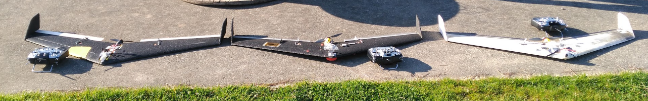 Figure 1
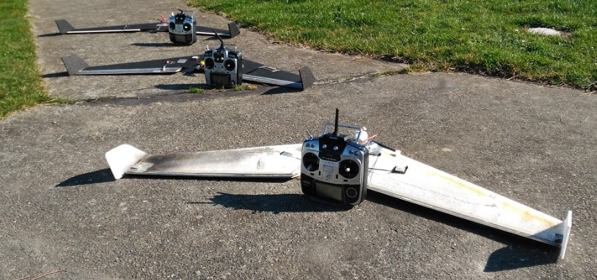 Figure 2
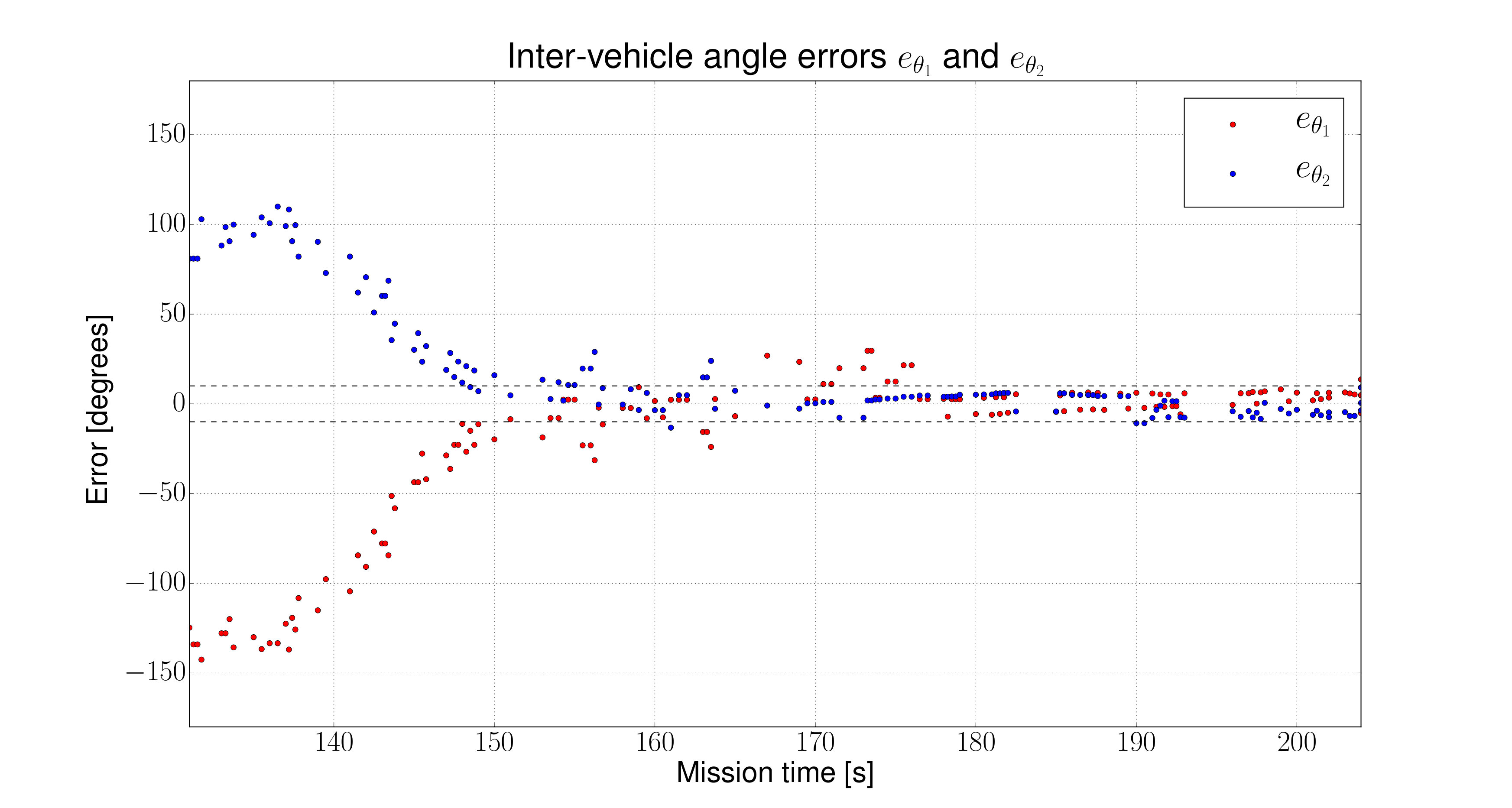 Figure 3
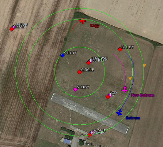 Figure 4
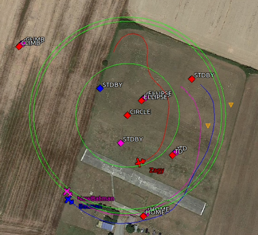 Figure 5
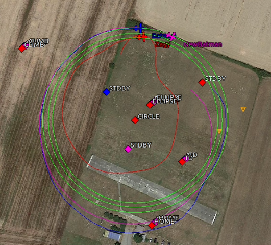 Figure 6
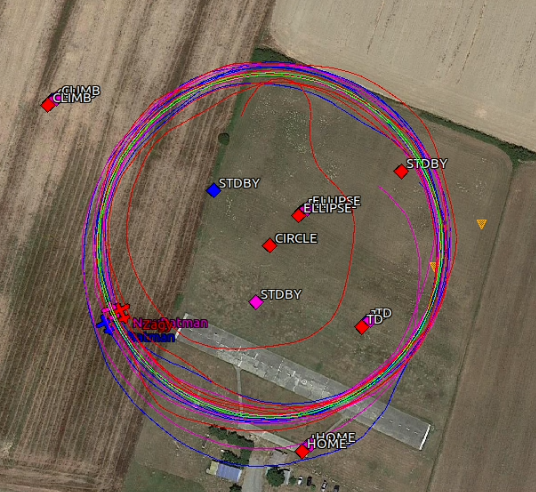 Figure 7
Peer Reviews
No public reviews on file for this paper yet. If you reviewed it on a platform where reviews are public (OpenReview, ICLR, NeurIPS, ICML), you can paste yours below so the community can read it here.
Videos
No videos yet. Explain this paper in a talk, walkthrough, or lecture? Add one.
Taxonomy
TopicsDistributed Control Multi-Agent Systems · Mathematical and Theoretical Epidemiology and Ecology Models · UAV Applications and Optimization
Circular formation control of fixed-wing UAVs with constant speeds.
Hector Garcia de Marina1 Zhiyong Sun2 Murat Bronz1 and Gautier Hattenberger1 1H. Garcia de Marina, M. Bronz and G. Hattenberger are with the Ecole National de l’Aviation Civile, University of Toulouse, Toulouse, France. [email protected].2Z. Sun is with the Australian National University, Canberra. [email protected].
Abstract
In this paper we propose an algorithm for stabilizing circular formations of fixed-wing UAVs with constant speeds. The algorithm is based on the idea of tracking circles with different radii in order to control the inter-vehicle phases with respect to a target circumference. We prove that the desired equilibrium is exponentially stable and thanks to the guidance vector field that guides the vehicles, the algorithm can be extended to other closed trajectories. One of the main advantages of this approach is that the algorithm guarantees the confinement of the team in a specific area, even when communications or sensing among vehicles are lost. We show the effectiveness of the algorithm with an actual formation flight of three aircraft. The algorithm is ready to use for the general public in the open-source Paparazzi autopilot.
I INTRODUCTION
There is a growing body of literature that recognises the importance of Unmanned Aerial Vehicles (UAVs) for aerial surveillance, search and rescue, patrol, inspection of facilities, precision agriculture, and atmosphere study [1, 2, 3]. The current trend in multi-agent systems [4] has led to a proliferation of works where individual and independent UAVs have gradually been replaced by a team of cooperative and coordinated ones [5, 6, 7, 8]. Formation control is one of the most well-known tools for assessing the cooperation and coordination of multi-agent systems [9, 10], where the usage of such a tool aims at forming and maintaining a prescribed geometrical shape for a group of vehicles.
An important challenge in the formation control of UAVs is to consider demanding constraints for the vehicles. For example, fixed-wing UAVs are preferred to rotorcrafts in missions where the endurance or the capacity for traveling long distances are essential requirements. However, rather than point mass models [11, 12], guidance algorithms for fixed-wing UAVs have to consider nonholonomic constraints, e.g., by modeling the aircraft as unicycles. Theoretical contributions on the coordination and formation control of unicycles include the consensus and rendezvous [13, 14], and the circular formations [15, 16]. The circular or pursuit formation design is a practical method for steering the vehicles to coordinated and periodic trajectories, which provide means to sample data with a desired spatial and temporal separation [17]. However, all the above mentioned works consider that both the speed and orientation of the vehicles can be actuated by the formation control algorithm in order to accomplish the mission’s goal.
Fixed-wing aircraft are usually designed for flying most efficiently at a given fixed airspeed [18]. Furthermore, an aircraft needs to fly with an airspeed over a certain lower bound or otherwise the aircraft stalls and falls down. Consequently, the control problem to be discussed in this paper considers unicycle-like vehicles with constant speed, i.e., we only actuate on the steering of the vehicle via coordinated turns by actuating on the bank angle of the aircraft. Note that having a constant airspeed does not imply to have a constant ground-speed because of the effect of the wind. Therefore, the wind causes the aircraft to travel with different ground speeds depending on its yaw and heading angles with respect to some frame of coordinates fixed on the ground, e.g., at center of the circular formation. Nevertheless, in this paper it will be assumed that the speed of the wind is much smaller than the desired airspeed, so the ground-speed can be considered almost constant during the vehicle’s mission.
Circular formations for unicycles with the constraint of having constant speeds make the formation control problem more challenging as it has been shown in the early work in [19] for just two vehicles. In particular, the analysis of constantly moving vehicles is problematic if one wants to control geometrical relations between them. However, a clever strategy consisting in controlling the instantaneous center of rotation of the vehicle, instead of its position, for a given fixed angular velocity has been employed in different works [20, 21, 22, 23, 24]. The benefit of this approach is that such instantaneous center of rotation for a unit speed vehicle can be fixed with respect to some global frame of coordinates while the vehicle is still moving, i.e., it just circulates around a constant point. The cited works applying this approach include the rendezvous of such points or the control of geometric relations between them such as position- or distance-based formation control approaches [9]. However, there are certain drawbacks associated with the control of such centers of rotation. For example, it is common that during the mission the steering control action of a vehicle could be close to or exactly zero. For such a situation, if communications or lines of sight for the sensors are lost, then the control action of the vehicle is not updated since the steering depends only on the relative states with respect to its neighbors, and consequently, the aircraft will continue flying straight. This is clearly a problem since nowadays the restrictions for drones in the airspace are tight in many countries. Therefore, the flight plan has to guarantee that the fixed-wing UAVs will not abandon their designated flying area.
In this paper we propose a distributed algorithm for controlling circular formations of fixed-wing UAVs with constant speeds, where each vehicle has a (feasible) prescribed inter-position with respect to its neighbors on the circle. In particular, the formation control algorithm does not directly actuate on steering the vehicle but setting the radius of the circle to be tracked by the vehicle, i.e., we actuate on the angular velocity of the vehicle around the center point of the circle. This approach can be related to algorithms where the agents are exclusively confined on the target circumference and they can change their phases [25, 26]. While several works controlling the inter-vehicle phases have considered constraints such as anonymity, restrictions in the communications or order preservation, to the best of the authors’ knowledge, only the work by Wang et al [27] addresses the constraint of having vehicles that cannot move backwards. However, such condition implies that the vehicles can be stopped on the circumference, something impossible for a fixed-wing aircraft.
The proposed algorithm in this work has a series of advantages and features. First, it is distributed, i.e., the vehicles depend only on relative measurements, such as relative positions, with respect to their neighbors, and a complete graph is not necessary. Second, unlike many of the above cited works, the desired inter-vehicle angles on the circle can be prescribed. Third, the desired formation is exponentially stable. Fourth, an arbitrary bound of the maximum distance of the vehicles with respect to the center of the circle can be chosen by design, therefore it is guaranteed the confinement of the formation regardless of broken communications or sensing. Fifth, it is possible to extend the algorithm to not only circles, but at least to any smooth closed orbit homeomorphic to a circle.
The remaining parts of the paper are organized as follows. In Section II, the notation, the considered model of the fixed-wing aircraft and the employed trajectory tracking algorithm for following a circle are introduced. In Section III we state the circular formation problem and propose the design of a controller as a solution together with a stability analysis. Experimental results with actual aircraft are presented in Section IV. The algorithm has been implemented in the popular open-source autopilot Paparazzi [28] and it is ready to be used by the general public.
II Preliminaries
II-A Notation
Consider a formation of fixed-wing UAVs whose positions are denoted by with . The vehicles are able to sense the relative positions with respect to their neighbors. The neighbors’ relationships are described by an undirected graph with the vertex set and the ordered edge set . The set of the neighbors of vehicle is defined by . Two vertices are adjacent if . A path from a vertex to a vertex is a sequence starting at and ending at such that two consecutive vertices are adjacent, and if then the path is called a cycle. We assume that the graph is connected, i.e., there is a path between any two vertices and . We define the elements of the incidence matrix , where denotes the cardinality of the set , for by
[TABLE]
where and denote the tail and head nodes, respectively, of the edge , i.e., .
A circular trajectory with radius can be described by the following implicit equation
[TABLE]
where and is a Cartesian position with respect to a frame of coordinates whose origin is at the center of . The plane can be covered by the following disjoint sets , where each level set is defined for a particular value of such that the resulting circle’s radius is non-negative, and in particular, the zero level set corresponds uniquely to . We define by the normal vector to the circle corresponding to the level set and the tangent vector at the same point is given by the rotation
[TABLE]
Note that belongs to the space and it is regular everywhere excepting at its center, i.e.,
[TABLE]
and all the level sets can be parametrized. In particular, the vehicle can calculate such parametrization associated to its position with the following expression
[TABLE]
Note that belongs to the circle group .
II-B Fixed-wing aircraft’s model
Consider for the unit speed ’th fixed-wing aircraft the following nonholonomic model in 2D
[TABLE]
where with being the attitude yaw angle111For our setup, the yaw angle and heading angle can be considered equal due to the absence of wind. and is the control action that will make the aircraft to turn. In particular, for coordinated turns where the altitude of the vehicle is kept constant and the pitch angle is close to zero, the control action corresponds to the following bank angle to be tracked by the autopilot of the vehicle
[TABLE]
where is the gravity acceleration.
II-C Trajectory tracking
One of the key points of the proposed formation control algorithm in this paper is to make sure that the aircraft is tracking . There exist many guidance algorithms in the literature [29, 30]. We have chosen the algorithm proposed in [31] that has been successfully tested in real flights [32] for two reasons. Firstly, the local exponential converge to the desired path is guaranteed. This property will help us later to support the convergence of the formation control algorithm under the argument of slow-fast dynamical systems in cascade. Secondly, the algorithm can be straightforwardly extended to other curves that are homeomorphic to , such as ellipses or the (possibly concave curve) Cassini ovals.
The trajectory tracking algorithm employs the level sets for the notion of error distance between the aircraft and . Note that for circular paths, the error has a clear relation with the Euclidean distance, but for more general trajectories, such as ellipses, this is not always true. The vehicle has to follow the vector field defined by
[TABLE]
where is a gain that defines how aggressive the vector field is, in order to converge to traveling on . Let us define as the unit vector constructed from the nonzero vector .
Theorem II.1
[31, 32]** Consider the system (5), then the control action
[TABLE]
where is the Hessian operator and , makes the aircraft to converge (locally) exponentially fast to travel over , i.e., for we have that with for some constants .
The first term in (8) makes the aircraft to stay on the guidance vector field (7) while the second term makes the vehicle to converge to the guidance vector field in case that the vehicle is not aligned with it.
III Circular formation control
III-A Problem definition
Given the neighbors’ relationship described by the graph , the stacked vector of inter-vehicle angles can be calculated as
[TABLE]
where (the -torus) is the stacked vector of parameters for each vehicle as in (4), and , therefore no necessarily all the inter-vehicle angles are calculated. Note that can be calculated from the relative measurement by just following trigonometric arguments in Figure 1. Consider a collection of desired on the circle. We define the formation error as the stacked vector of signals
[TABLE]
where . The objective of the proposed algorithm for the team of fixed-wing UAVs in the next subsection is to achieve simultaneously and as .
III-B Controller design and stability
Consider that the unit speed aircraft is tracking correctly , therefore its angular velocity around the center of is
[TABLE]
The idea is to control the inter-vehicle angles in by changing in the vehicles the desired trajectory to be tracked, i.e., instead of (2), the vehicle has to track
[TABLE]
where is the formation control signal to be designed and the superindex denotes for the vehicle . Note that the smaller the (possibly negative), the bigger the radius of , and thus the smaller the angular velocity . For the sake of simplicity in the following analysis we define
[TABLE]
where is a control action with a more straightforward physical meaning than , i.e., we set the radius (around the desired ) of the circumference (or simply ) because
[TABLE]
Remark III.1
Note that for a generic closed trajectory, if a vehicle tracks it on a negative level set, then it travels less distance than one that tracks the same trajectory on a positive level set after one loop.
We propose the following control action for achieving the desired circular formation
[TABLE]
where stands for the ’th row of the incidence matrix as in (1), and . Since , we impose to the following condition
[TABLE]
i.e., we avoid the possibility of setting a negative radius222Note that while a level set can be negative, the radius of a circumference cannot. in . Note that the control action (15) is based on the popular consensus algorithm in formation control [9].
Before presenting the main result, we need the following technical lemma that will define the neighbors’ relationships.
Lemma III.2
If does not contain any cycles, then the matrix is Hurwitz.
Proof:
If does not contain any cycles, it has been show in [33] that for any nonzero vector . Note that , implying that is positive definite. Hence, is Hurwitz if does not contain any cycles. ∎
We also make use of the following assumption.
Assumption III.3
A vehicle is always tracking and traveling over as in (12).
The Assumption III.3 considers that if there is a change in the radius of , then the vehicle instantaneously jumps to the required level set. As we will show, the circular formation controller (15) guarantees the exponential stability of the origin of the error signal under the Assumption III.3. Since the trajectory error tracking in Theorem II.1 is also locally exponentially stable, one may consider a slow-fast dynamics in cascade by tuning appropriately the gains and in (7) and (15) respectively [34, Chapter 4]. Informally, the controller (8) provides a fast transient process of the vehicle to if the aircraft is sufficiently close to it, while the whole formation slowly follows the formation controller (15). In fact, if is sufficiently small, the set of possible trajectories will be very close to , therefore making reasonable the Assumption III.3. Furthermore, since for circles the convergence of the algorithm in Theorem II.1 is almost globally stable (with the exception of starting at the center of ), even if the vehicles start far away from the trajectories to be tracked, they will approach a situation where Assumption III.3 can eventually be considered.
Theorem III.4
Consider a team of unit speeds aircraft modeled as in (5), and the graph defining the neighbors’ relationships does not contain any cycles. All the vehicles are tracking (12) by employing (8). If Assumption III.3 holds and the level sets in (12) are controlled by (15) via (13), then the origin of the error as in (10) is locally exponentially stable for the desired .
Proof:
The proof is based on checking the stability of the linearization of the error dynamics around the origin. First note that . According to Assumption III.3, we also have that for each edge the agents and are tracking a circle of radius and respectively, so from (11) it holds that
[TABLE]
where is the ’th row of the matrix as in Lemma III.2. We linearize (17) around , therefore the dynamics of small variations of the error are given by
[TABLE]
which leads to the following compact form
[TABLE]
and because is Hurwitz according to Lemma III.2 since has not any cycles, we can conclude that the equilibrium is locally exponentially stable. ∎
Remark III.5
Note that since the convergence to the trajectories is asymptotic, one can guarantee that all the vehicles will be confined in a disc of radius , which corresponds to the worst case radius to be tracked, for all time , even if the control is not updated, e.g., the vehicles are not exchanging or sensing their positions.
It is interesting to highlight that if does not contain any cycles, then in such a disc the only equilibrium point for the system is at , which has been proven stable. Since the vehicles are eventually confined in according to Theorem II.1, it seems reasonable to conjecture that an estimation of the region of attraction for the exponentially stable is indeed . Furthermore, for a proof of the convergence of the overall system without Assumption III.3, one can use the stability theory of cascade systems [34, Chapter 4], while the exponential stability of the partial system (17) could guarantee the (locally) asymptotic stability of the overall system. We will present a rigorous proof in the extended journal version.
IV Implementation and flight performance
IV-A Experimental platform
The validity of Theorem III.4 has been tested with the three fixed-wing UAVs shown in Figure 2. The aircraft have about grams of weight, m of wingspan, and they are actuated by two elevons and one motor. The electronics include a battery that allows about minutes of autonomy at the nominal flight, which corresponds to an airspeed of m/s. The chosen board for running the Paparazzi autopilot stack is the Apogee [35], which includes the usual sensors of three axis gyros, accelerometers, magnetometers. Each fixed-wing UAV has on board an U-Blox GPS with a nominal accuracy of meters in the horizontal plane. The airplanes exchange their positions according to , so they can compute the corresponding inter-vehicle angles . The source code can be checked online at the Paparazzi repository [35].
IV-B Circular formation flight experiment
The formation flight333The video of the experiment with HD quality can be watched at https://www.youtube.com/c/HectorGarciadeMarina . has been taken place at the aero model club of Eole at Muret, close to the city of Toulose in France. The flights were performed on the 17th of February, 2017 between the 10:00 and the 12:00 hours local time. The wind coming from the south was about m/s according to MeteoFrance, therefore we can consider that ground-speed and airspeed are approximately equal. The airplanes and are tagged with the colors blue, pink and red respectively at the ground station captions in Figure 3. The chosen incidence matrix for the communication between vehicles is
[TABLE]
which clearly does not define any cycles. The desired formation is defined by , i.e., all the aircraft achieve consensus for their corresponding . Potential collisions are avoided by making the airplanes to fly at different altitudes, which are and meters above the ground for planes and respectively. The target circle is set at the waypoint CIRCLE in Figure 3 with a desired radius equal to meters. The gains and in Theorems II.1 and III.4 have been set to and respectively. The airplanes exchange their positions with a frequency of Hz, although lost communications are expected. Note that each airplane has a different understanding of , i.e., each airplane calculates on board the error signal and it might be different among neighbors due to lost communications or GPS delays. Interesting work studying the effects of this fact in formation control can be found at [36, 37].
Before the formation control algorithm begins the three aircraft are orbiting at different standby points. The experiment starts at time seconds in Figure 3. At this moment the algorithm commands the airplane (red) to follow a circumference with a much smaller radius than airplanes (blue) and (pink) in order to catch them up. In fact, airplanes and are tracking a circumference with a bigger radius than in order to wait for airplane . In about seconds, the errors have been reduced half. Some lost communications have been experienced between times and seconds. However, the algorithm seems robust against such an issue and the formation achieves consensus within a band of degrees of error, and continues stable until the end of the experiment after seven laps.
V Conclusions
This paper has presented an algorithm for achieving circular formations with fixed-wing UAVs traveling with constant speeds. The strategy consists in controlling the angular velocities around the center of the desired circle. For that, we design a control action that is applied to the level set to be tracked around the desired circle. These level sets are tracked by a guidance vector field algorithm that is locally exponentially stable. Since the presented algorithm for circular formations is also exponentially stable if the vehicles are perfectly tracking the level sets, we employ the argument of slow-fast systems in cascade in order to show the compatibility of both algorithms, which has been demonstrated in practice with three aircraft. The algorithm can be potentially extended to other closed non-circle trajectories. A more rigorous analysis will be presented in an extension of this work.
The reference list from the paper itself. Each links out to its DOI / PubMed record.
- 1[1] R. W. Beard, T. W. Mc Lain, D. B. Nelson, D. Kingston, and D. Johanson, “Decentralized cooperative aerial surveillance using fixed-wing miniature UA Vs,” Proceedings of the IEEE , vol. 94, no. 7, pp. 1306–1324, 2006.
- 2[2] M. A. Goodrich, B. S. Morse, D. Gerhardt, J. L. Cooper, M. Quigley, J. A. Adams, and C. Humphrey, “Supporting wilderness search and rescue using a camera-equipped mini UAV,” Journal of Field Robotics , vol. 25, no. 1-2, pp. 89–110, 2008.
- 3[3] P. Tokekar, J. Vander Hook, D. Mulla, and V. Isler, “Sensor planning for a symbiotic UAV and UGV system for precision agriculture,” IEEE Transactions on Robotics , vol. 32, no. 6, pp. 1498–1511, 2016.
- 4[4] R. Olfati-Saber, J. A. Fax, and R. M. Murray, “Consensus and cooperation in networked multi-agent systems,” Proceedings of the IEEE , vol. 95, no. 1, pp. 215–233, 2007.
- 5[5] A. Ryan, M. Zennaro, A. Howell, R. Sengupta, and J. K. Hedrick, “An overview of emerging results in cooperative UAV control,” in Decision and Control, 2004. CDC. 43rd IEEE Conference on , vol. 1. IEEE, 2004, pp. 602–607.
- 6[6] L. Bertuccelli, M. Alighanbari, and J. How, “Robust planning for coupled cooperative UAV missions,” in Decision and Control, 2004. CDC. 43rd IEEE Conference on , vol. 3. IEEE, 2004, pp. 2917–2922.
- 7[7] X. Wang, V. Yadav, and S. Balakrishnan, “Cooperative UAV formation flying with obstacle/collision avoidance,” IEEE Transactions on control systems technology , vol. 15, no. 4, pp. 672–679, 2007.
- 8[8] D. M. Stipanović, G. Inalhan, R. Teo, and C. J. Tomlin, “Decentralized overlapping control of a formation of unmanned aerial vehicles,” Automatica , vol. 40, no. 8, pp. 1285–1296, 2004.