On the Selection of Calculable Residual Generators for UAV Fault Diagnosis
Georgios Zogopoulos-Papaliakos, Kostas J. Kyriakopoulos

TL;DR
This paper presents a methodology for selecting calculable residual generators for UAV fault diagnosis, combining prior and posterior information to efficiently identify minimal cost, implementable residuals in structural analysis.
Contribution
It introduces a novel approach that integrates a priori and a posteriori data to improve the selection process of residual generators for UAV fault detection.
Findings
Reduced time to find implementable residual generators
Effective application to UAV fault diagnosis
Enhanced reliability of structural analysis methods
Abstract
Structural Analysis is an established method for Fault Detection and Identification (FDI) in large-scale systems, enabling the discovery of Analytical Redundancy Relations (ARRs) which serve as residual generators. However, most techniques used to enumerate ARRs do not specify the matching used to calculate each of those ARRs. This can result in non-implementable or unusable residual generators, in the presence of non-invertibilities in the equations involved or in lack of computational tools. In this paper, we propose a methodology which combines a priori and a posteriori information in order to reduce the time required to find implementable, usable residual generators of minimum cost. The method is applied to a fixed-wing Unmanned Aerial Vehicle (UAV) model.
Click any figure to enlarge with its caption.
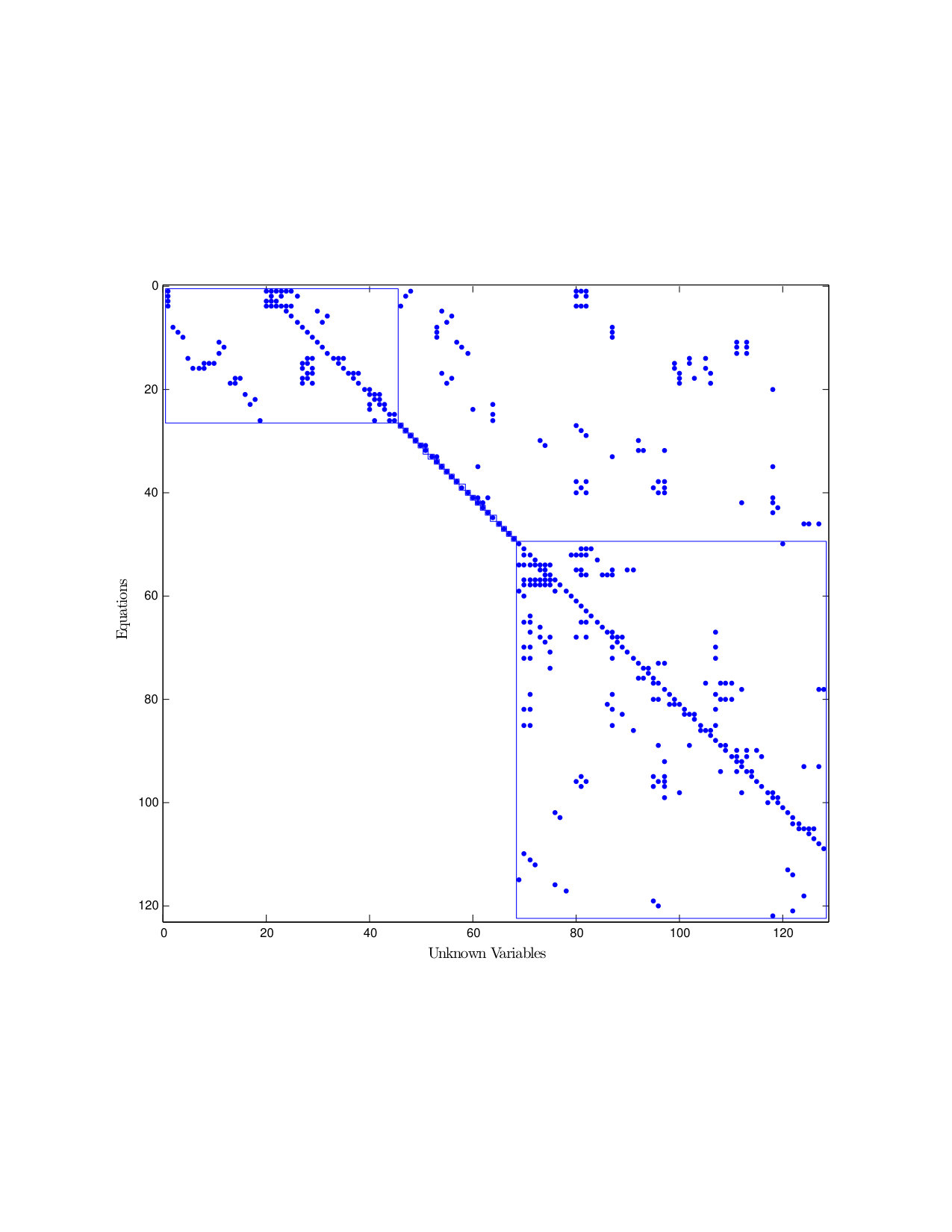 Figure 1
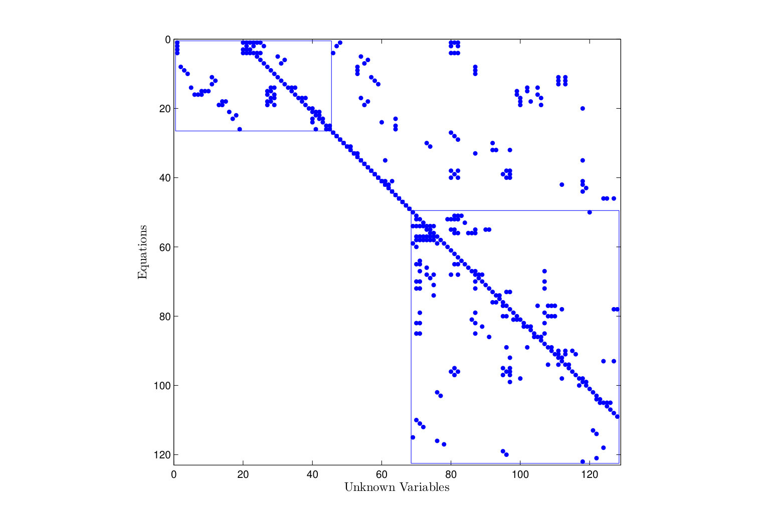 Figure 2
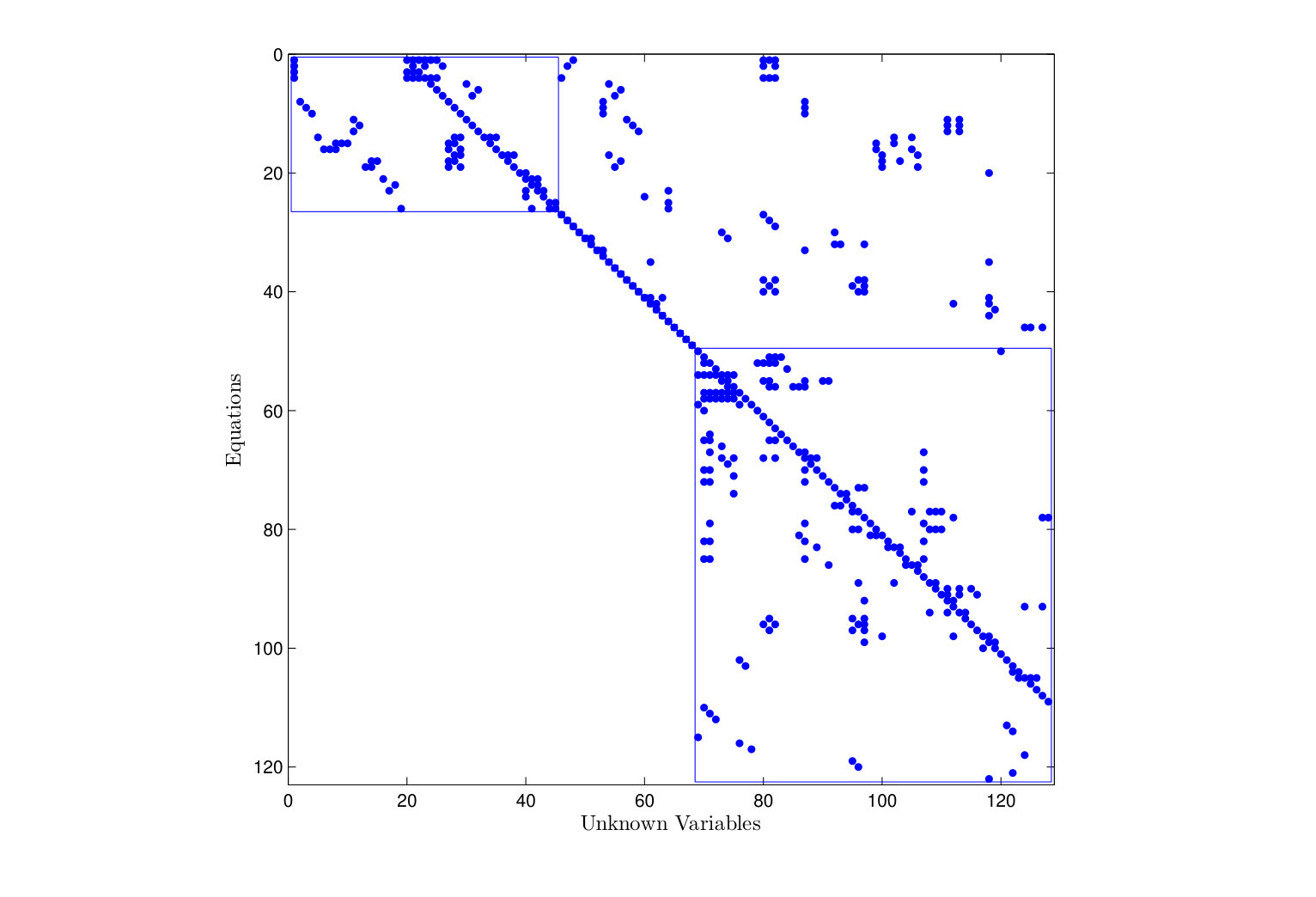 Figure 3
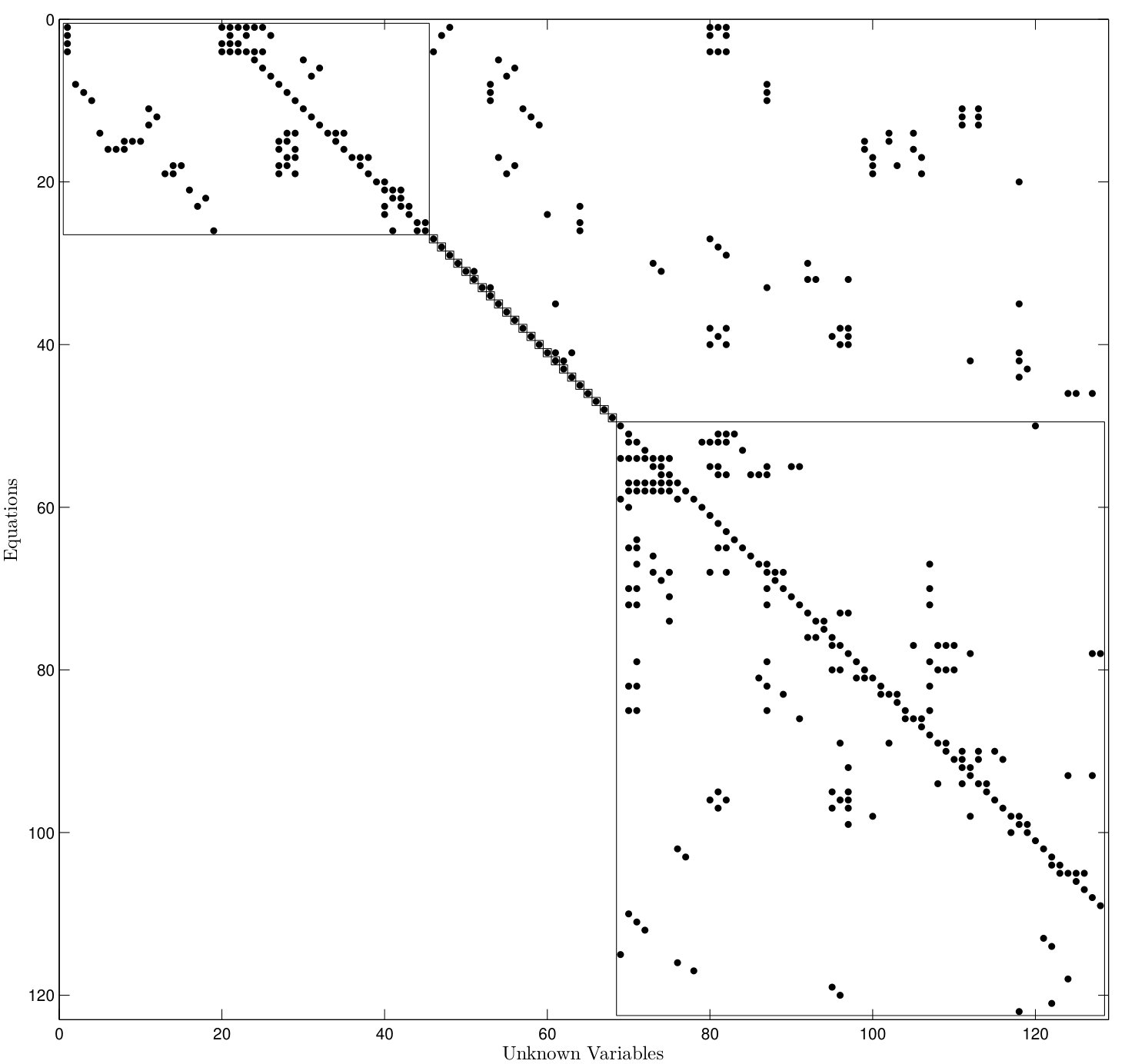 Figure 4
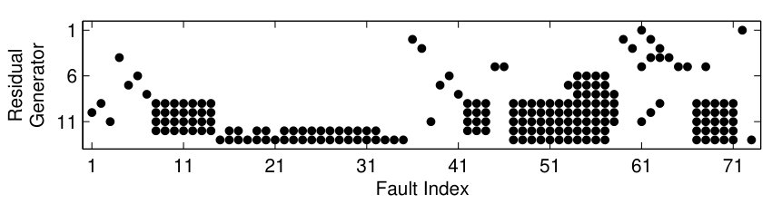 Figure 5
| Generator | s26 | d1 | d2 | k4 | m2 | k6 | k5 |
|---|---|---|---|---|---|---|---|
| Cost | 2 | 3 | 3 | 4 | 6 | 205 | 206 |
| Generator | k7 | k2 | k1 | k3 | f12 | f12 | |
| Cost | 206 | 1356 | 1356 | 1556 | 2206 | 2218 |
Peer Reviews
No public reviews on file for this paper yet. If you reviewed it on a platform where reviews are public (OpenReview, ICLR, NeurIPS, ICML), you can paste yours below so the community can read it here.
Videos
No videos yet. Explain this paper in a talk, walkthrough, or lecture? Add one.
On the Selection of Calculable Residual Generators for UAV Fault Diagnosis
Georgios Zogopoulos Papaliakos and Kostas J. Kyriakopoulos The authors are with Control Systems Lab, School of Mechanical Engineering, National Technical University of Athens, Greece {gzogop, kkyria}@mail.ntua.gr
Abstract
Structural Analysis is an established method for Fault Detection and Identification (FDI) in large-scale systems, enabling the discovery of Analytical Redundancy Relations (ARRs) which serve as residual generators. However, most techniques used to enumerate ARRs do not specify the matching used to calculate each of those ARRs. This can result in non-implementable or unusable residual generators, in the presence of non-invertibilities in the equations involved or in lack of computational tools. In this paper, we propose a methodology which combines a priori and a posteriori information in order to reduce the time required to find implementable, usable residual generators of minimum cost. The method is applied to a fixed-wing Unmanned Aerial Vehicle (UAV) model.
I INTRODUCTION
Even though there exist well-established algorithms for the control of commercial Unmanned Aerial Vehicles (UAVs), they are rarely designed to handle faults. Notably, faults are most common in commercial UAVs, since such vehicles are manufactured to lower quality standards, compared to military and aerospace applications.
A fault is a deviation of the system parameters or the system structure from the nominal condition. Most of the times, if faults are allowed to go unchecked, they will eventually result to failures, rendering the system inoperable. Hence, it is important to detect faults as early as possible and take counter-measures against them, in order to maintain system health and ensure its operational status.
It is reasonable to expect from modern UAVs to exhibit fault-tolerance to a certain degree and, to that goal, Fault Detection is indispensable. Fault Detection involves setting up mathematical and physical structures that are able to detect when a fault occurs in a system. Afterwards, Fault Isolation can be performed, in order to identify the system component which is under fault. This is an important piece of information, since it allows us to locate the source and nature of a fault [1].
In consistency-based diagnosis for continuous-time systems, the difference between a measured quantity and a quantity estimate based on the nominal system behaviour is used to perceive faults. Under no-fault conditions, should hold and vice versa. Such difference functions are called residuals. Ultimately, a residual can be formulated as , i.e. as a function of continuous-time measurements. is called a residual generator function. The required information to perform FDI can be provided either by hardware redundancy or analytical redundancy. The first approach places multiple, redundant sensory equipment on the aircraft which contribute in validity checks. However, this is not a lucrative option in small UAVs, where low weight, cost and power consumption are desired features. Thus, the second approach, where redundant information is introduced by mathematical models, stands out as a prominent field of research. Finding Analytical Redundancy Relations (ARRs) which can be used as residual generators is a primary goal [1, 2, 3].
In order to perform model-based FDI at the component level, it is necessary to enumerate and take into account the equations which make up the mathematical model of the UAV down to that level. However, such detailed representations will yield hundreds of equations, rendering the process of finding consistency checks very hard to do by hand. Formal, scalable methods are required to achieve this. Structural Analysis (SA) provides such methods [1, 4] and has been used in linear systems [5]. Still, SA is not yet able to extract consistency checks for generic, non-linear systems automatically as well as in real-time, a prerequisite for UAS with high autonomy and reconfigurable controllers.
In this paper, we propose a methodology reducing the time needed to perform the residual selection task, by using a weighted bipartite graph structure and combining information available both a priori and a posteriori of the analysis.
In section II, SA is presented in the context of residual generator extraction. In section III, limitations in current SA techniques are mentioned. In section IV, we introduce the concept of a weighted structural graph. In section V, our proposed methodology is expanded upon. In section VI, an application example on a fixed-wing UAV model is presented. Finally, section VII concludes this work.
II STRUCTURAL ANALYSIS
SA is a qualitative modeling methodology which, given a mathematical model, captures only whether there exist relations between equations (also referred to as constraints) and variables. The resulting structure, although abstract, provides information on component interaction and facilitates FDI methods. The structure can be represented as a bipartite graph and graph-theoretic methods can be used to extract results in a methodical manner [1],[4].
II-A The Structural Model
We construct the set of model constraints , with elements , corresponding to each of the equations comprising the mathematical model of our system. In this work, we choose to expand by adding the differentiation constraints separately for all differentiated variables, instead of inserting differentiated versions of existing constraints; we treat a variable and its derivative as structurally different [1]. Given the set of available model constraints , we construct the structural model of the system in the form of an undirected bipartite graph [1, 4, 6]. is the set of involved variables, composed by the set of known variables (such as inputs and measurements) and the set of unknown variables . We can write that , and to denote all, known and unknown variables in . is the set of edges connecting and , .
A bipartite graph can also be represented as a biadjacency matrix, whose rows correspond to constraints and columns to variables. The biadjacency matrix is defined as
[TABLE]
Without loss of structural information we can use only to populate the columns.
II-B Solving the System Graph
While searching for ARRs, it is of interest to solve as many equations for one of their variables as possible. Structurally, this is equivalent to assigning each variable vertex to one constraint vertex, respecting the edge set. The notion of matching of a graph is very useful for that purpose.
Matching is a subset of such that [7], i.e. given the set of edges , we select edges so that no two edges have a common vertex. If the cardinality of is the maximum possible for a given , then the matching is called maximal. If or , then the matching is called complete with respect to or to respectively. If then the matching is perfect. For a given graph, the maximal matching may not be unique. Unless the matching is complete on , then no variable in is guaranteed to be calculable.
After a matching has been found, we can create a directed graph , with its edges defined as \mathcal{E}_{d}{=}\{e_{i,j}{=}(c_{i},x_{j})$$:$$e_{i,j}{\in}\mathcal{M}\} \{e_{i,j}{=}(c_{i},x_{j})$$:$$(x_{j},c_{i}){\notin}\mathcal{M}\}, . The reverse of this graph is obtained by reversing the directionality of its edges and is denoted as .
Definition 1** (Reachability)**
Given an undirected (directed) graph and two vertices , is reachable from iff there is an undirected (directed) path in from to . A subset is reachable from iff there is an undirected (directed) path from to . A subset is reachable from subset iff there is an undirected (directed) path from to , .
For any given bipartite graph, a unique decomposition on is defined, called the Dulmage-Mendelsohn (DM) decomposition. It identifies three (possibly empty) subgraph components: , and . The decomposition guarantees that there exists a complete matching on in , a perfect matching in and a complete matching on in . Thus, is called the under-constrained part of , just-constrained and over-constrained [8]. The decomposition can take a block-triangular form (Figure 1). The diagonal line represents the matchings between and .
Since fault detection uses analytical redundancy in the form of unmatched constraints, which exist only in it is evident that the only faults that can be detected are those which affect constraints belonging in .
II-C Matching Algorithms
There are several matching algorithms for undirected bipartite graphs, but two of them are the most common in SA applications.
The first one is the Ranking algorithm, which was presented in [1] and propagates an ”information front” based on known variables. It has the property that every constraint it matches has exactly one variable unknown at that time, which is then solved for. The complexity of this algorithm is O() [9]. It is fast and can easily produce an acyclic calculation order, but cannot guarantee a complete matching when applied on cyclic graphs.
Another, more classical algorithm is the Hungarian method. The original algorithm [10] and its multiple improvements [11] have been a standard tool in graph theory and specifically for calculating maximum matchings in undirected bipartite graphs. They have low, polynomial computational cost, and are applicable for weighted undirectional graphs as well. They can extract maximal matchings for cyclic graphs but may contain cycles.
II-D MSOs
Each unmatched constraint in can be used as residual generator to detect faults in equations reachable from , in . In order to minimize the fault candidates for each triggered residual, it is of interest to find residuals which are sensitive to as few faults as possible.
The notion of Minimal Structurally Overdetermined sets (MSOs) is useful for that purpose [6]. An MSO is a set of equations whose corresponding graph has the following properties:
2. 2.
3. 3.
4. 4.
With a slight abuse of notation, we will denote the corresponding graph of an MSO, as .
From each MSO we can extract different residual generators, one for each . The rest of the equations in form a just-constrained system for which a perfect matching can be found. This matching provides a calculation method for all the variables used by that residual generator. It should be noted that the number of possible MSOs grows exponentially large with the number of redundant equations in the initial system [6].
In order to reduce the number of candidate MSOs, it is beneficial to consider only MSOs with at least one equation which can fail. A residual generator which involves only constraints which cannot fail is not useful and clutters the residual selection procedure [12].
III Causality and Calulability
The previously mentioned structural methods, regarding the selection of residual generators in large scale systems, provide only best-case results. During the creation of the structural graph crucial information is lost and structural analysis may yield residual generators which are unusable or at least, non-optimal according to certain criteria.
Factors which can affect the feasibility and quality of the extracted residual generators are presented in this section. Namely, we will focus on the topics of causality, calculability and calculation cost.
III-A Causality
Given an analytical equation, we might deny the ability to solve it for a specific variable. Such a decision might stem from poor sensitivity, the existence of multiple solutions or simply the absence of an inverse function.
The existence of dynamic equations raises another concern, regarding the ability of the actual, automated FDI system to perform either numerical differentiation or integration [13, 9]. If our FDI system has the ability to perform numerical differentiation but not integration, then it is said that it operates under differential causality. If the inverse is true, e.g. due to unacceptable noise amplification, it is said that it operates under integral causality. The combination of the above, which allows for both differentiations and integrations is called mixed causality [14]. Differential and integral causalities pose restrictions in the admissible structural graph edges which can be incorporated in a matching set.
Causality restrictions can be applied and visualized by adding directionality in the related edges of the graph, resulting in a partially-directed causal bipartite graph . Yet, this poses a serious limitation, since most computationally cheap matching tools are applicable only to undirected bipartite graphs.
III-B Calculability
The available computational solution tools also pose a constraint to the admissible matchings. Differentiators and integrators have already been mentioned in the previous subsection, but more types exist. The DM decomposition of any just-constrained system may yield König-Hall components of size larger than 1, as seen in Fig. 1, denoted by . Any matching spanning those components will produce a directed graph with cycles, also known as Strongly Connected Components (SCCs). Since equations belonging in the same cycle have to be solved simultaneously, simultaneous equation solver tools must be available [14, 15]. If a König-Hall component contains only linear equations, then a Linear Algebraic Equation solver is required. If it contains at least one non-linear algebraic equation, then a Nonlinear Algebraic Equation solver is required. If it contains at least one dynamic equation, then a Differential Equation solver is required. Thus, depending on the available tool set in our FDI system, some matchings may be rejected.
III-C Additional Issues
Even under differential (or mixed) causality, differential edges which belong in a loop (i.e. cycle) cannot be part of a calculable matching: Differential Equation solvers propagate the state variables by integration, not differentiation [16]. Also, even under mixed causality, for practical applications, it is not desirable to add integral edges in a matching when they do not belong in a König-Hall component, i.e. they are edges in a path of ; noise bias will quickly invalidate the integration result. We propose the term calculation causality to capture the above restrictions.
The final remark concerns the Ranking matching algorithm, which is a lucrative algorithm thanks to its low computational cost. As mentioned, the Ranking method is not guaranteed to find a complete matching on in cyclic graphs. However, it is worth considering since there are cases where it can produce complete matchings, as seen in Fig. 2.
IV A Weighted Graph Approach
As was previously mentioned, matching a variable with a constraint implies solving the constraint for that variable. It may be easier, from a computational standpoint, to solve one constraint for one of its variables than for another. Encoding this kind of information in the structural model in the form of weighted edges provides a compact and easily manipulable data structure, which can then be used to discourage matchings of high computational cost and shorten the iteration time of a real-time FDI system. The costing information can be encoded in the structural graph in the form of edge weights. Let an edge be assigned with a weight , via the weight function , representing the cost of solving constraint for variable .
Let there be a graph with a perfect matching , a weight function and a variable .
Definition 2** (Matching Cost)**
The cost of the matching is
[TABLE]
Definition 3** (Residual Generation Cost)**
Let there be a residual generator , the matching-induced graph and its inverse . Let the reachable variable set from in be . Take the subset . The cost of the residual calculation is:
[TABLE]
where is the evaluation cost of a residual generator from its variables.
In [2] a weight function was used to compare residual generators, but by pricing the operators in the analytical residual generator expression, not the structural graph edges.
A comparison among matching costs can be done in several levels:
Each residual is assigned a residual generation cost, which constitutes a selection criterion for the composition of the FDI scheme. 2. 2.
Within , for residual generator , comparing matching costs for all feasible matchings can lead to the selection of the cheapest calculation order. Let that cost be . 3. 3.
Within , comparing the cheapest matching cost of each potential residual generator produces the cheapest residual generator for . Let that cost be .
The actual costing information may be derived from computer science resources, engineering expertise or symbolic mathematics software.
Commonly in computing systems, addition and subtraction are of equal computational cost, multiplication is less ten times more expensive, division is about ten times more expensive and trigonometric functions and powers are almost 100 times more expensive. Square root cost varies with implementation but is generally expensive.
Regarding causality, edges which imply integration can be assigned greater cost, since integration requires storage space to hold the integrator state. Differentiation may be assigned an even greater cost, since it has the undesired effect of noise amplification.
Finally, information on sensor noise can be inserted in the structural graph by weighting corresponding edges proportionally to the noise variance of the corresponding sensor discouraging the use of a high-noise sensor.
V Proposed Residual Generation Method
Existing methods perform post-processing of results to obtain maximal, calculable matchings of minimum cost in cyclic graphs. That requires the whole set of possible matchings be enumerated and then post-processed. This is problematic, since the number of different possible matchings grows exponentially with the number of vertices. Even by examining the over-constrained part only, the problem of choosing out of constraints to match variables of equal number can yield as many as matchings [3]. MSOs help reduce the number of candidate matchings, but the pool can still remain significantly large.
We propose a method for shortening the time required to produce the set of candidate residual generators and select the optimal ones, through a combination of a priori and a posteriori graph processing.
V-A Step 1: DM Decomposition
Conventionally, a DM decomposition is applied on the undirected system graph to extract the over-constrainted part. This provides the best-case detectability possibilities.
V-B Step 2: A Priori Matching Propagation
Next, a maximal, calculable, loop-less matching of minimum cost is sought. Weights are applied to graph edges, as was discussed in the previous section. For this step, differential causality is enforced to avoid open-loop integrations. The Weighted Elimination matching algorithm is introduced to find a matching with the aforementioned properties. This algorithm is similar to the Ranking algorithm, in that it matches a variable to a constraint only if all the other variables of that constraint are known.
is the pool of candidate matching extensions . In line 3 is initialized. While there exist candidate matching extensions (line 4), the cost contribution of each new matching extension is calculated (line 5). The matching extension with the smallest cost is selected (line 6) and added to the matching. The selected matching extension is removed from , along with other candidate extensions that would match the same variable (line 10). New, feasible matching extensions are added to and the loop repeats. inline]Investigate on the naming ”elimination”
After WeightedElimination is completed, some unmatched constraints with all of their variables matched may exist. These constitute residual generators and are added to the candidate residual generator pool.
inline]Present the algorithm properties
V-C Step 3: A-Posteriori Matching Selection
Commonly, König-Hall blocks will exist and WeightedElimination will not return a maximal matching. The variables which are matched so far are considered known and the remaining subgraph can now be searched for MSOs.
Each MSO is searched for the cheapest, calculable residual generator evaluation. In order to find the minimum cost matching efficiently, we implemented Murty’s algorithm [17] to obtain all possible matchings in order of increasing cost.
The algorithm GetOptimalResidual finds the cheapest, calculable residual generator expression which respects calculability constraints for a given .
The function Murty returns the set of all the perfect matchings of the provided just-constrained graph, sorted by increasing cost. IsCalculable is given a just-constrained graph, a matching and a set of solver tools and answers whether this matching can be calculated based on those tools.
GetOptimalResidual is given an MSO set and for every candidate residual generator (line 2) it uses Murty to obtain all perfect matchings in ascending cost. The first calculable matching is selected (line 6). Once all residual generators have been examined, the one with the smallest cost is selected for the input MSO (line 13).
As matchings are examined in increasing cost order, if at least one calculable matching exists for the residual generator , it is found in at most iterations and the cheapest residual will be available in at most iterations, where is the number of constraints in said MSO.
Each MSO is examined and one residual generator is extracted from it. Afterwards, residual generators are selected in ascending cost order, until the specified detectability or isolability criteria are met.
VI Application Example
A dedicated Matlab class for graph representation and manipulation was created, preserving the partially directed graph structure instead of the biadjacency matrix representation, which cannot hold directionality information.
VI-A The System Model
We applied the proposed method on the mathematical model of a fixed-wing UAV, comprized of 122 equations and 162 variables. The equations describe a multitude of submodels, ranging from the standard rigid-body kinematics, to aerodynamics, to propeller dynamics, to electric motor dynamics, to sensor models. In total, there are 26 equations denoted as for the rigid body kinematics, 48 equations for the rigid body dynamics, 13 equations state explicitly the differentiated states, 6 equations for the atmosphere model and 29 equations for the measured quantities. A full equation list wouldn’t fit in this paper.
Out of the complete equation set, we allowed only 58 equations to be subject to faults. Namely, , , , , , , , , .
We evaluated the addition and subtraction operations with a weight of 1 cost unit, multiplication with 5, division with 10, roots, powers, and trigonometric functions with 100, integration with 100 and differentiation with 200. The weight assigned to each edge is equal to the total cost of the corresponding mathematical expression.
We assumed that integrators, differentiators, linear, non-linear and differential equations systems solvers were available.
VI-B Results
Initially, DM decomposition of the undirected system graph was performed, as shown in Fig. 3.
26 equations and 45 unknown variables belong to the under-constrained part, 23 equations and unknown variables belong to the just-constrained part and 73 equations and 60 unknown variables belong to the over-constrained part. Thus, out of the possible 58 faults, only the 34 ones which correspond to can be detected in the best case.
By applying the WeightedElimination algorithm to the resulting over-constrained part, we were able to match 42 variables and 50 equations. The 8 extra equations were assigned as candidate residual generators. The remaining graph is of much smaller size, and hence, lower complexity.
Then, we extracted all the MSO sets from the remaining graph. The analysis showed that out of 350 MSOs, 349 involved equations with potential faults. The cheapest, feasible residual generators of each MSO were stored, along with their corresponding cost.
The residual selection criterion was maximum detectability, but maximum isolability would be valid as well. In increasing cost order, the residual generators which extended fault detectability of the FID system were chosen. Table I shows the resulting fault signatures matrix.
In total, 13 residual generators were needed to achieve full fault detectability. Their costs are presented in Table II.
Two selected residuals are presented in detail. Residual generator uses only 2 matching edges to evaluate the residual. The reachable subgraph from , involving equations and does not form any loops, hence no simultaneous equation solving tools are required to calculate the residual. This expected, since this residual generator was found during the application of WeightedElimination.
The affecting equations, involving part of a GPS sensor measurements are:
[TABLE]
where is the Northwards position. This residual generator can be used to monitor the GPS sensor health.
[TABLE]
Another residual generator is . It was found during the MSO search phase and spans both the initial matching produced by WeightedElimination as well as the matching selected for its MSO. 28 equations are involved in its calculation: 8 as part of the MSO (, , , , , , , ) and the rest as part of the initial matching (, , , , , , , , , , , , , , , , , , ).
The constraints which where matched during WeightedElimination can be calculated by substitution. The remaining 8 equations need to be solved simultaneously.
[TABLE]
-, and are part of the standard rigid-body kinematics equation set. - are measurements from a 3-axis accelerometer, solved for the force component. This is a dynamic system which can be solved by a differential equations solver.
VII Conclusions
In this paper, SA methods were employed to perform fault diagnosis in large-scale systems. Previous similar works were presented, which employed graph-theoretical methods to investigate the existence of analytical redundancy relations used as residual generators for fault diagnosis. Yet, those approaches did not take into account the implementation issues stemming from either causality restrictions, or calculability problems, or the existence of sets of simultaneous equations.
We introduced a method for finding causal, calculable residual generators of minimum cost, based on a novel, weighted bipartite graph representation. The combination of a priori and a posteriori information allows us to produce results in reduced time.
We applied the proposed method onto an example, large-scale model of a fixed-wing UAV and showed that different types of residual generators can be obtained, depending on the specified search criteria.
The reference list from the paper itself. Each links out to its DOI / PubMed record.
- 1[1] M. Blanke, M. Kinnaert, J. Lunze, and M. Staroswiecki, Diagnosis and fault-tolerant control , 2nd ed. Springer Berlin Heidelberg, 2006.
- 2[2] M. Fravolini, V. Brunori, G. Campa, M. Napolitano, and M. La Cava, “Structural Analysis Approach for the Generation of Structured Residuals for Aircraft FDI,” IEEE Transactions on Aerospace and Electronic Systems , 2009.
- 3[3] M. Krysander and J. e. a. Aslund, “An Efficient Algorithm for Finding Minimal Overconstrained Subsystems for Model-Based Diagnosis,” IEEE Transactions on Systems, Man, and Cybernetics , 2008.
- 4[4] R. Izadi-Zamanabadi, “Structural analysis approach to fault diagnosis with application to fixed-wing aircraft motion,” in Proceedings of the 2002 American Control Conference , 2002.
- 5[5] T. Boukhobza, F. Hamelin, and C. Simon, “A graph theoretical approach to the parameters identifiability characterisation,” International Journal of Control , 2013.
- 6[6] M. Krysander and J. Aslund, “An Efficient Algorithm for Finding Over-constrained Sub-systems for Construction of Diagnostic Tests,” in 16th International Workshop on Principles of Diagnosis) , 2005.
- 7[7] K. Murota, Matrices and matroids for systems analysis . Springer, 2000.
- 8[8] a. L. Dulmage and N. S. Mendelsohn, “Coverings of bipartite graphs,” Canadian Journal of Mathematics , 1958.