Effect fusion using model-based clustering
Gertraud Malsiner-Walli, Daniela Pauger, Helga Wagner

TL;DR
This paper introduces a Bayesian model-based clustering method for effect fusion in categorical variables, enabling automatic grouping of levels with similar effects to improve regression analysis.
Contribution
It proposes a novel Bayesian prior that encourages effect fusion and uses model-based clustering during MCMC to identify similar effect levels and irrelevant variables.
Findings
Effective in simulation studies for grouping effects
Identifies non-influential variables automatically
Improves effect estimation accuracy in high-dimensional data
Abstract
In social and economic studies many of the collected variables are measured on a nominal scale, often with a large number of categories. The definition of categories is usually not unambiguous and different classification schemes using either a finer or a coarser grid are possible. Categorisation has an impact when such a variable is included as covariate in a regression model: a too fine grid will result in imprecise estimates of the corresponding effects, whereas with a too coarse grid important effects will be missed, resulting in biased effect estimates and poor predictive performance. To achieve automatic grouping of levels with essentially the same effect, we adopt a Bayesian approach and specify the prior on the level effects as a location mixture of spiky normal components. Fusion of level effects is induced by a prior on the mixture weights which encourages empty components.…
Click any figure to enlarge with its caption.
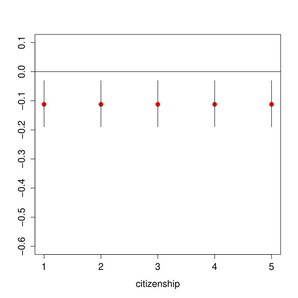 Figure 1
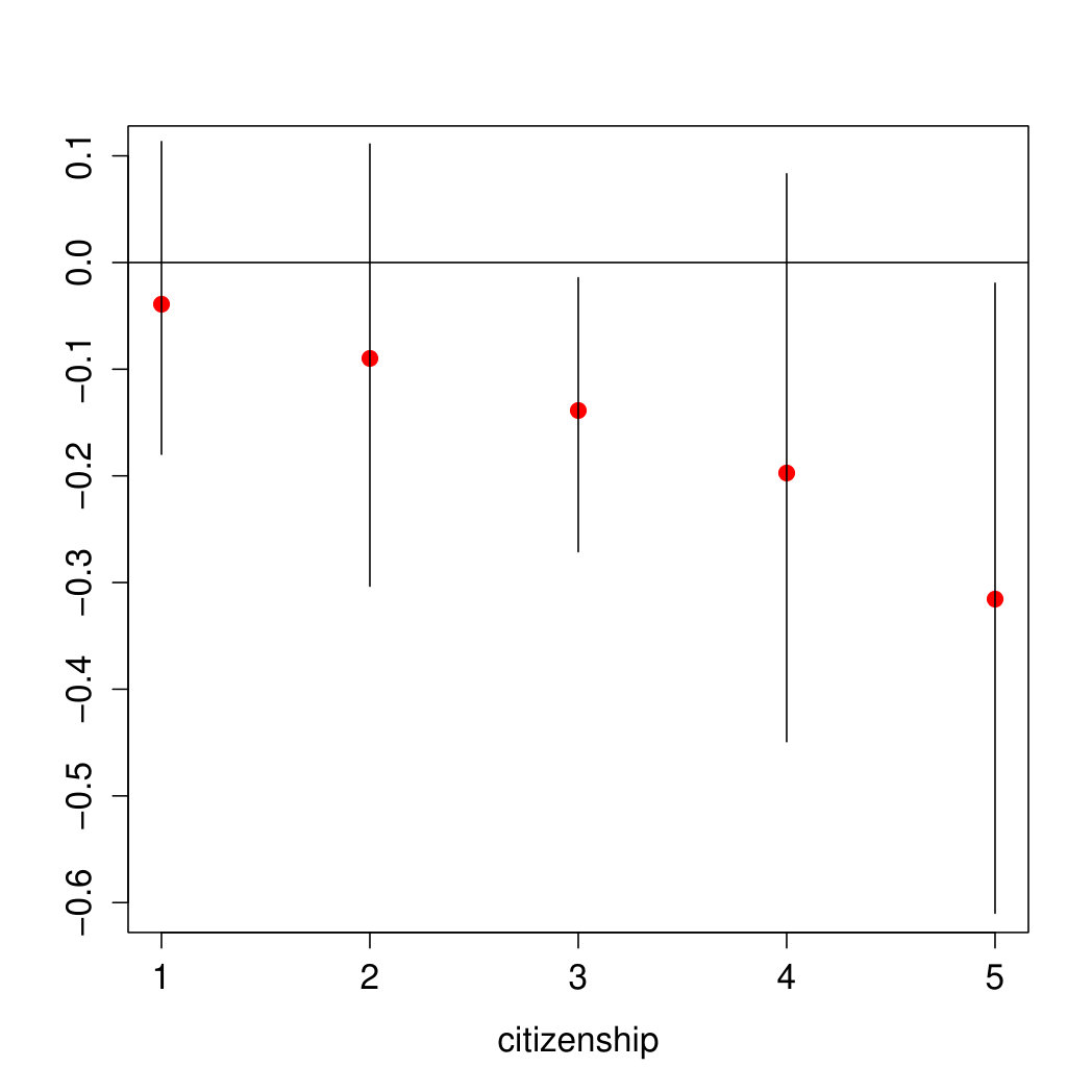 Figure 2
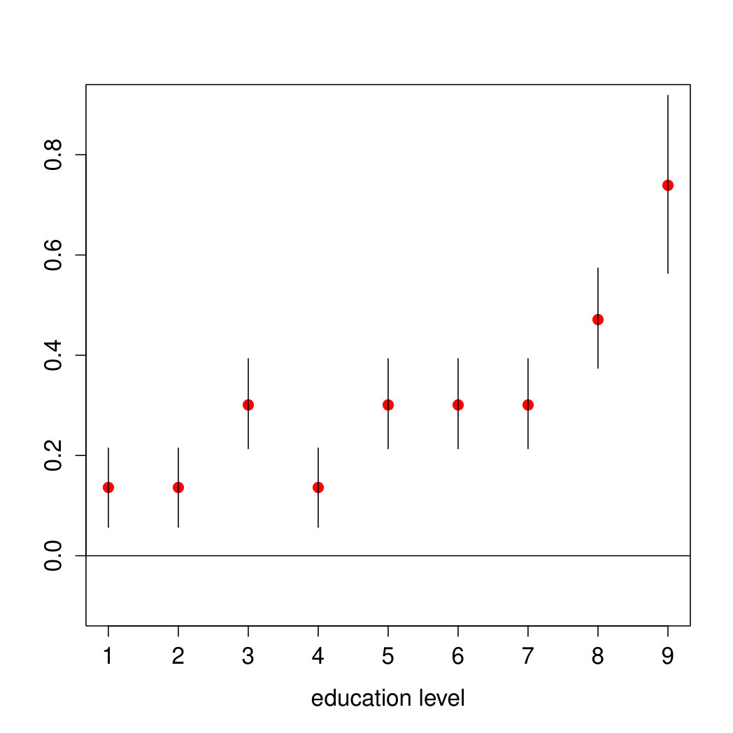 Figure 3
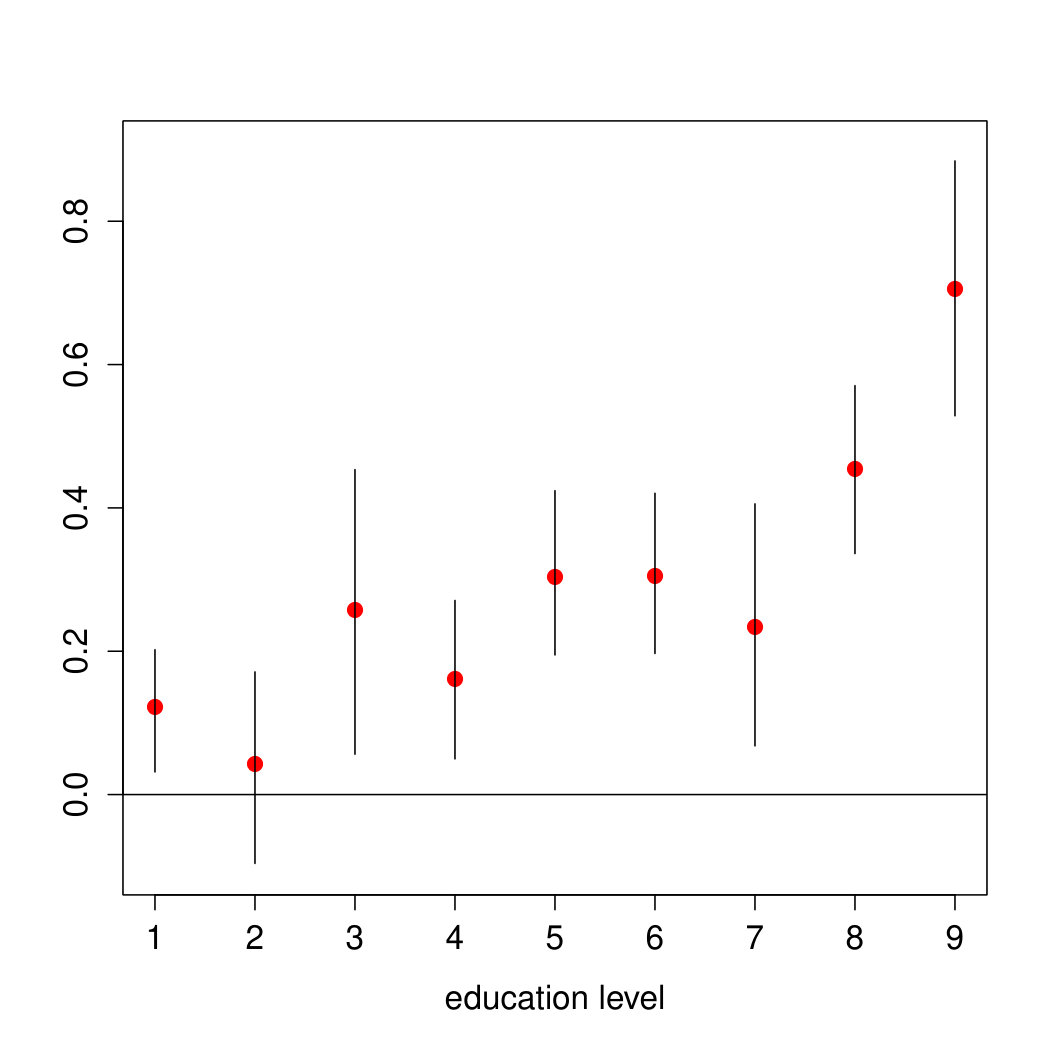 Figure 4
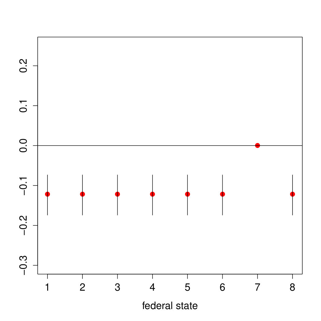 Figure 5
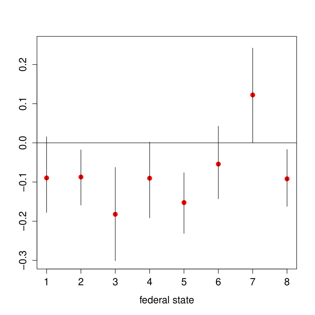 Figure 6
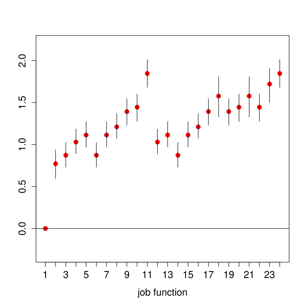 Figure 7
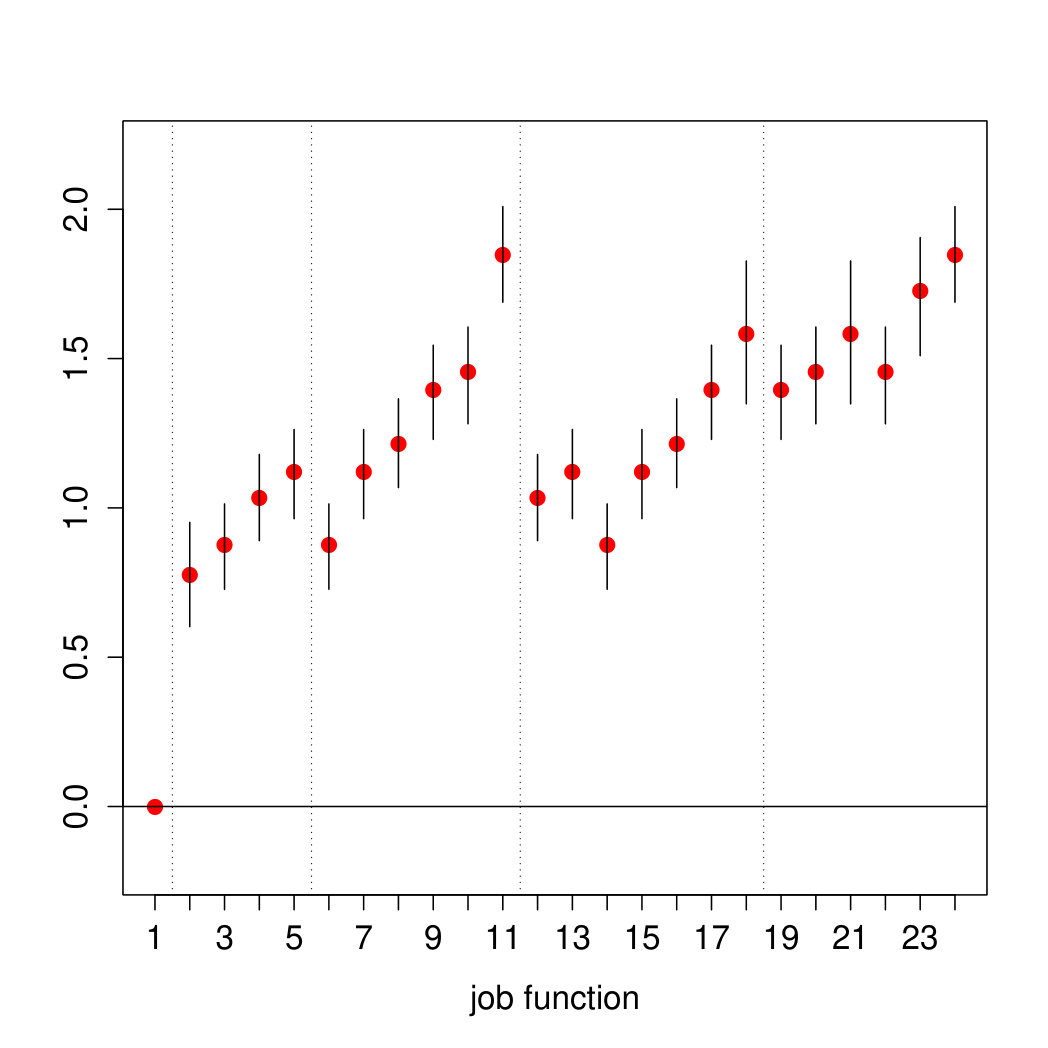 Figure 8
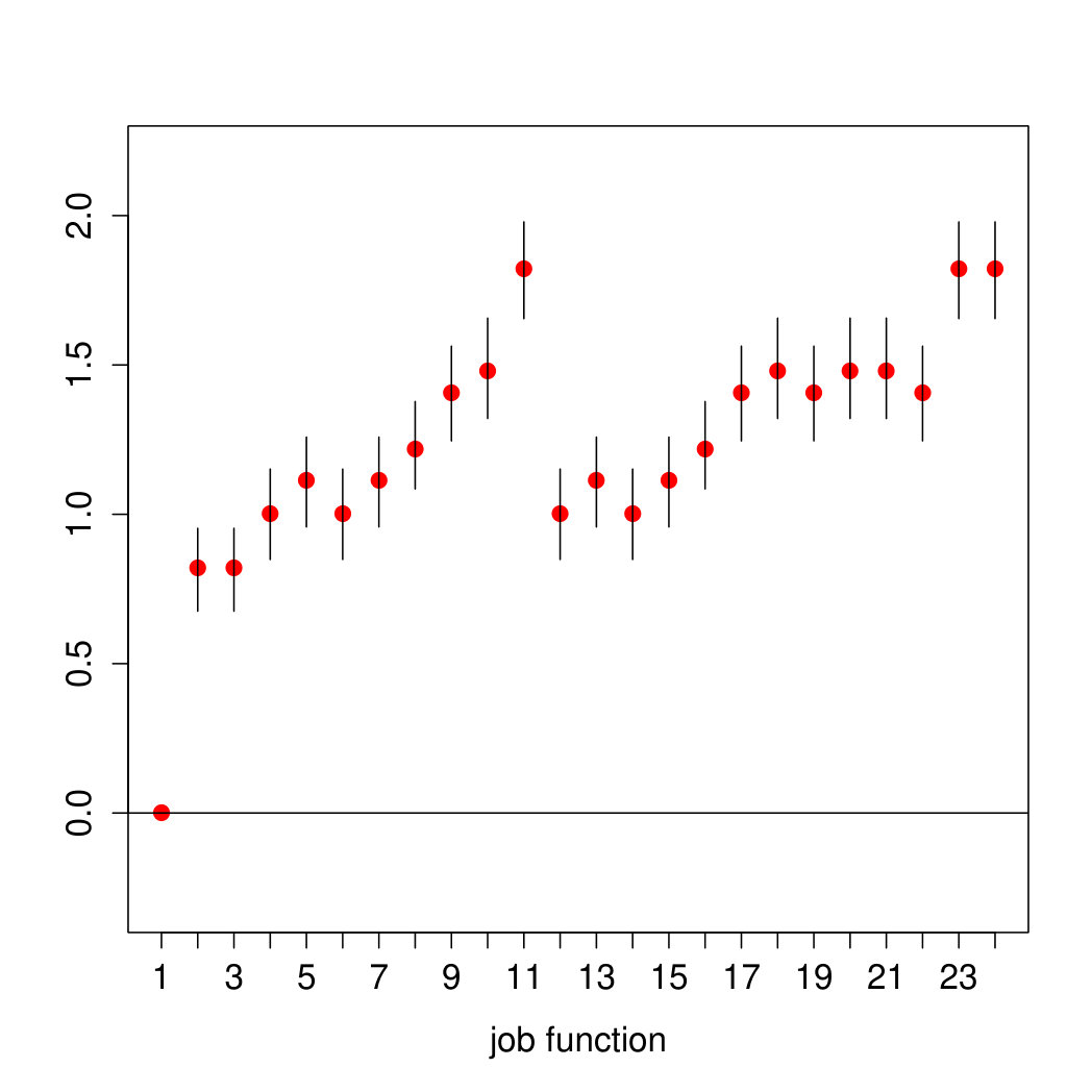 Figure 9
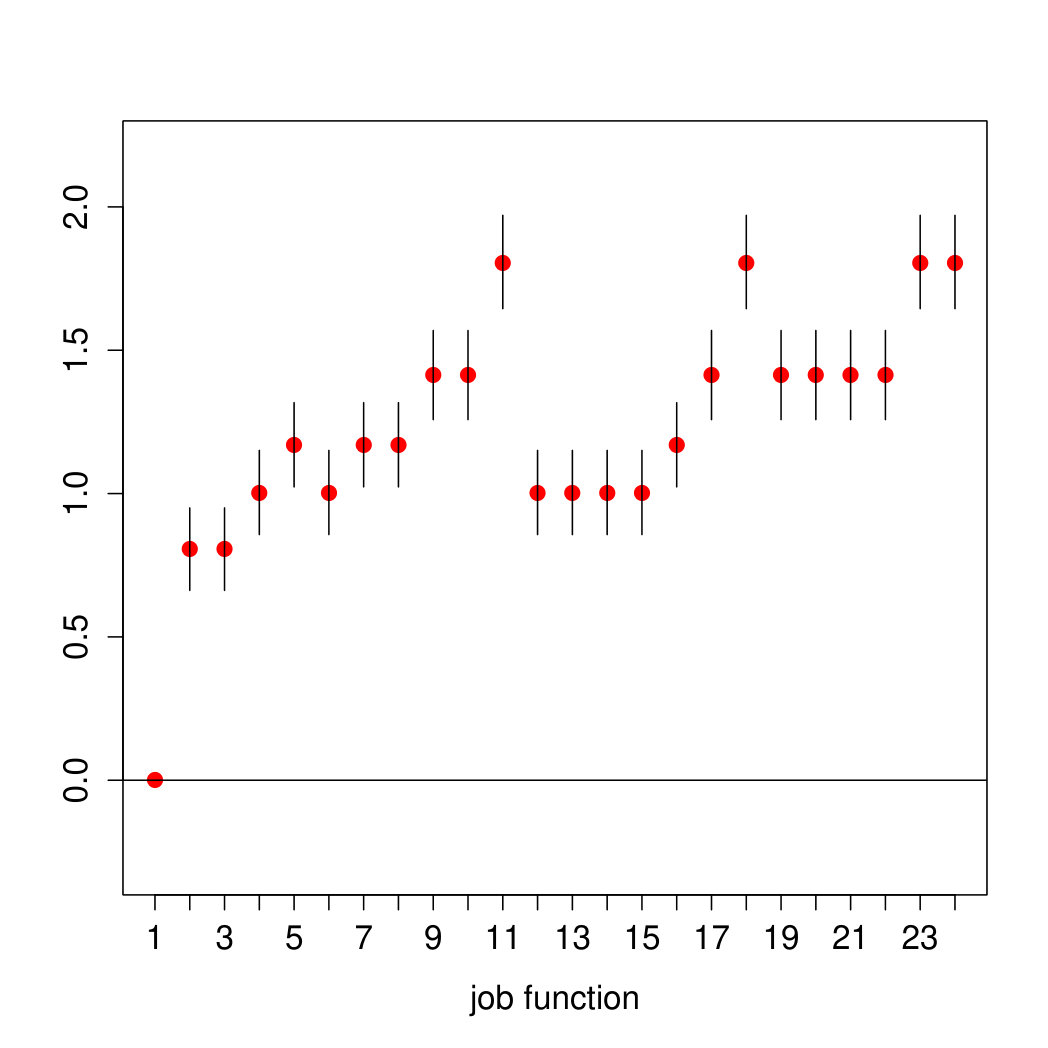 Figure 10
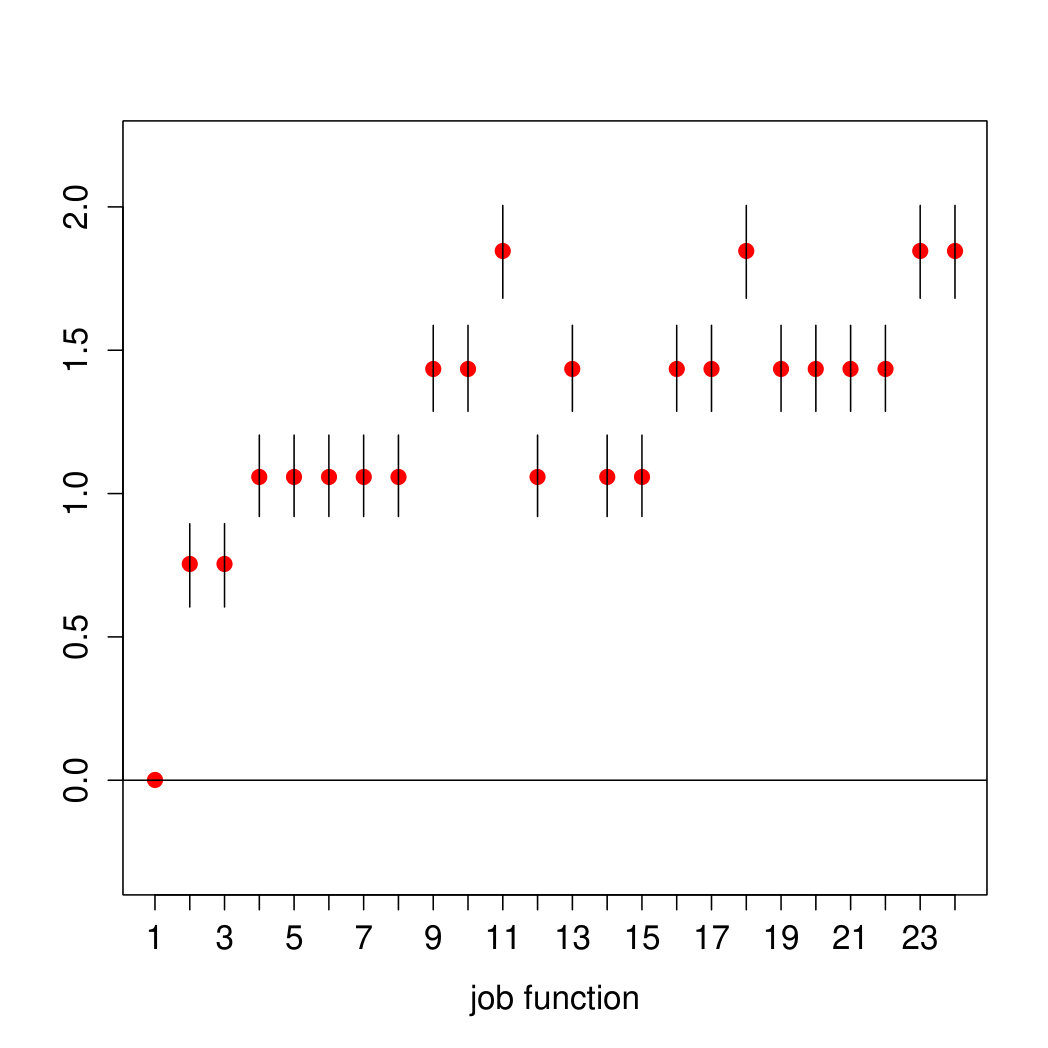 Figure 11
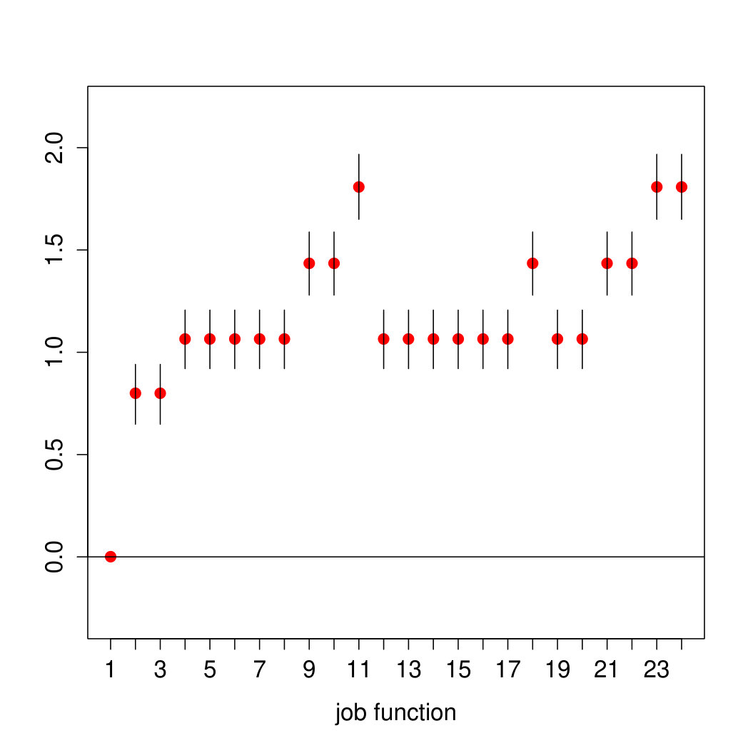 Figure 12
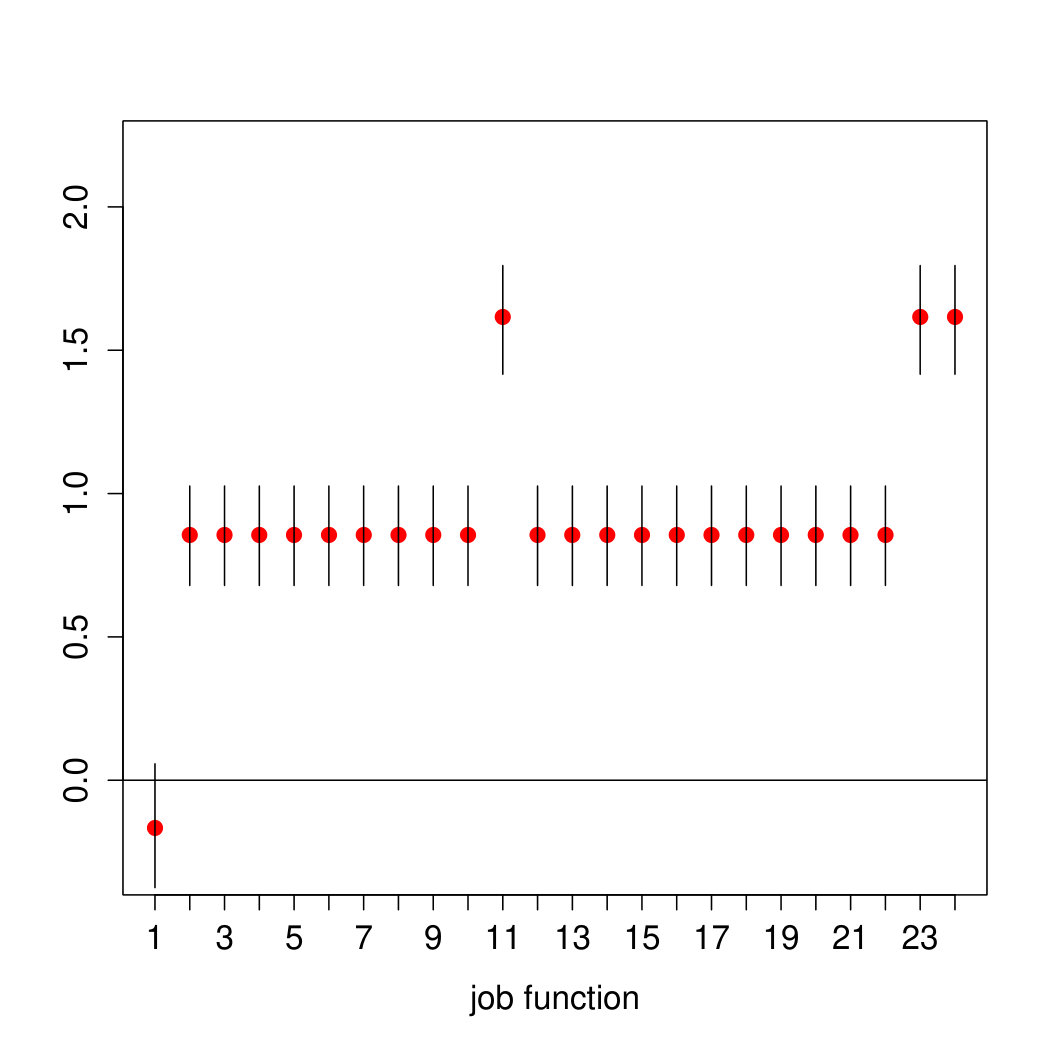 Figure 13
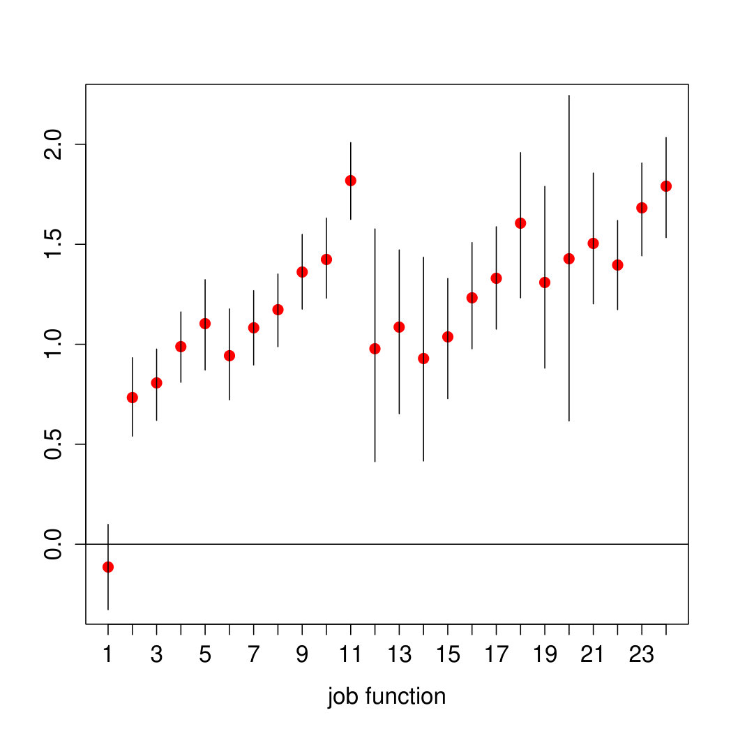 Figure 14
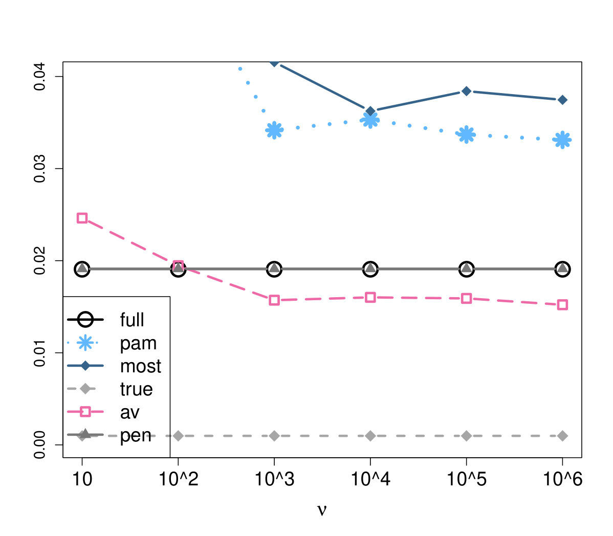 Figure 15
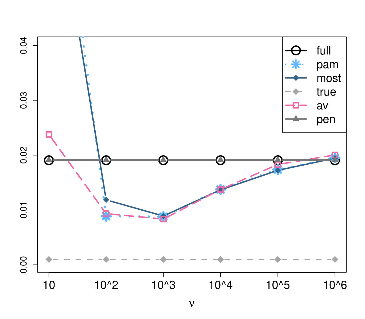 Figure 16
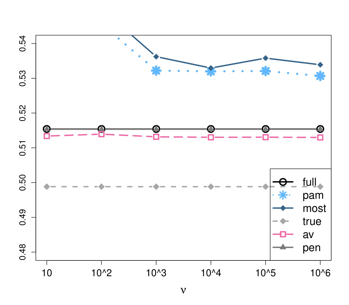 Figure 17
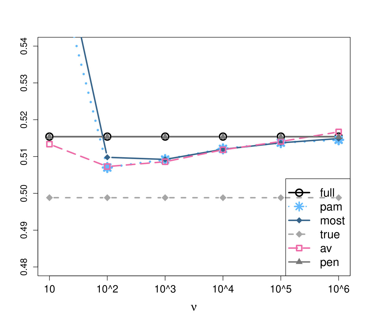 Figure 18
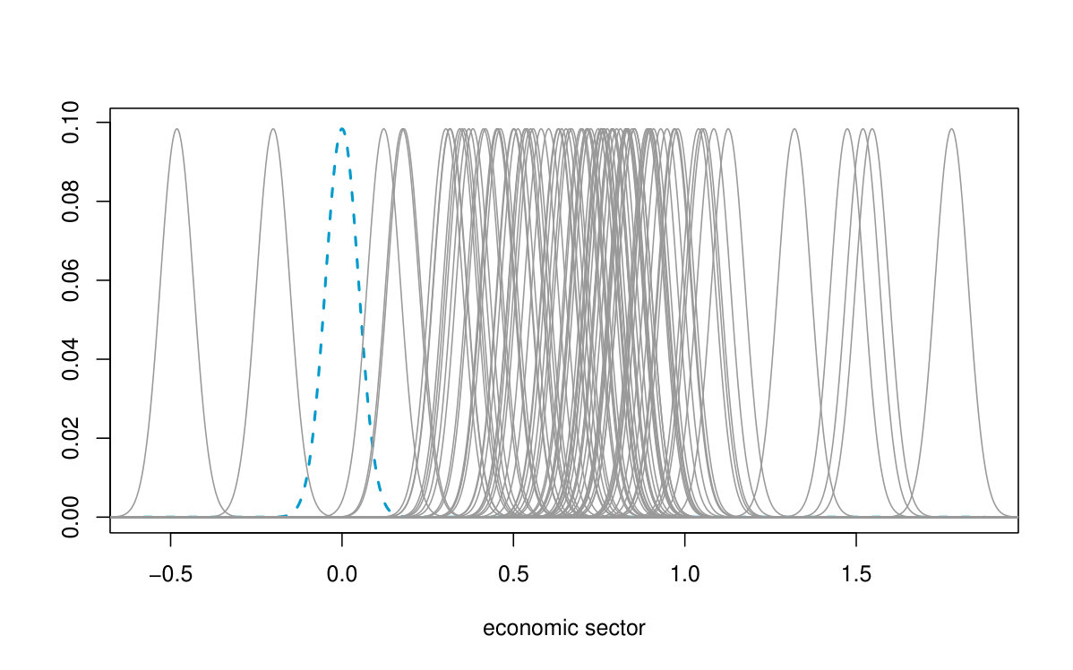 Figure 19
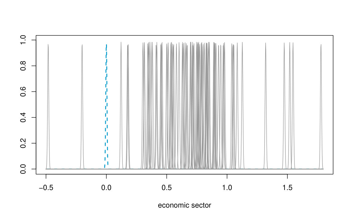 Figure 20
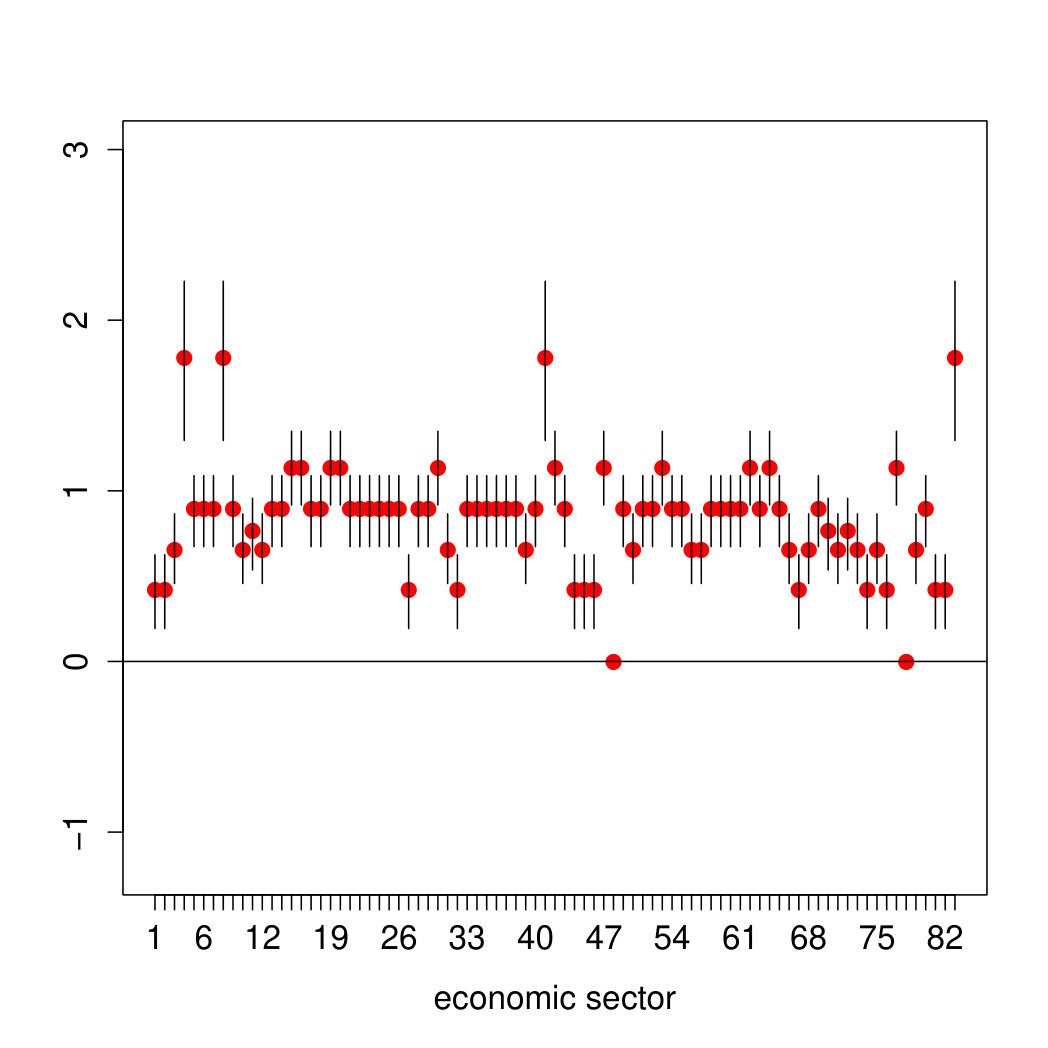 Figure 21
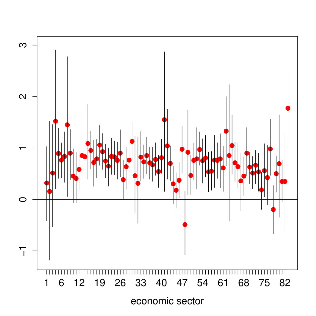 Figure 22
| Variable | freq | groups | AR | err | FPR | FNR | ||||||
|---|---|---|---|---|---|---|---|---|---|---|---|---|
| true | most | pam | most | pam | most | pam | most | pam | most | pam | ||
| 1 | 14844 | 3 | 3.0 | 3.0 | 1.00 | 1.00 | 0.00 | 0.00 | 0.00 | 0.00 | 0.00 | 0.00 |
| 2 | 14970 | 2 | 2.0 | 2.0 | 1.00 | 0.99 | 0.00 | 0.00 | 0.00 | 0.00 | 0.00 | 0.00 |
| 3 | 11897 | 1 | 1.8 | 2.0 | 0.26 | 0.00 | 0.23 | 0.28 | 0.33 | 0.41 | - | - |
| 4 | 11044 | 6 | 6.0 | 6.2 | 0.91 | 0.90 | 0.04 | 0.04 | 0.08 | 0.08 | 0.02 | 0.02 |
| Var | true | groups | AR | err | FPR | FNR |
|---|---|---|---|---|---|---|
| 1 | 3 | 9.0 | 0.12 | 0.60 | 0.91 | 0.00 |
| 2 | 2 | 7.7 | 0.03 | 0.66 | 0.92 | 0.00 |
| 3 | 1 | 7.2 | 0.00 | 0.74 | 0.92 | - |
| 4 | 6 | 59.8 | 0.05 | 0.83 | 0.96 | 0.01 |
| freq | groups | AR | Error | FPR | FNR | |||||||
|---|---|---|---|---|---|---|---|---|---|---|---|---|
| most | pam | most | pam | most | pam | most | pam | most | pam | |||
| fixed | 10 | 9 | 3.8 | 3.4 | 0.52 | 0.53 | 0.49 | 0.49 | 0.06 | 0.04 | 0.21 | 0.20 |
| 54 | 6.1 | 6.1 | 0.91 | 0.93 | 0.04 | 0.03 | 0.07 | 0.06 | 0.02 | 0.01 | ||
| 11044 | 6.0 | 6.2 | 0.91 | 0.90 | 0.04 | 0.04 | 0.08 | 0.08 | 0.02 | 0.02 | ||
| 8077 | 6.7 | 7.0 | 0.87 | 0.86 | 0.09 | 0.09 | 0.14 | 0.15 | 0.02 | 0.01 | ||
| 7159 | 11.0 | 11.6 | 0.69 | 0.68 | 0.28 | 0.30 | 0.40 | 0.42 | 0.01 | 0.01 | ||
| 6800 | 19.6 | 20.6 | 0.46 | 0.44 | 0.50 | 0.53 | 0.65 | 0.68 | 0.00 | 0.00 | ||
| random | 10 | 9 | 3.7 | 3.4 | 0.52 | 0.53 | 0.49 | 0.49 | 0.06 | 0.04 | 0.21 | 0.20 |
| 46 | 4.2 | 4.3 | 0.62 | 0.64 | 0.35 | 0.30 | 0.07 | 0.10 | 0.14 | 0.12 | ||
| 38 | 4.7 | 4.8 | 0.70 | 0.73 | 0.26 | 0.21 | 0.06 | 0.09 | 0.11 | 0.08 | ||
| 42 | 4.9 | 4.9 | 0.73 | 0.73 | 0.24 | 0.21 | 0.06 | 0.09 | 0.09 | 0.08 | ||
| 44 | 4.8 | 4.9 | 0.72 | 0.73 | 0.25 | 0.21 | 0.05 | 0.09 | 0.10 | 0.08 | ||
| 45 | 4.8 | 4.9 | 0.72 | 0.74 | 0.24 | 0.20 | 0.06 | 0.09 | 0.10 | 0.08 | ||
| BICmcmc | DIC | ||||
| most | pam | most | pam | ||
| true | 8501 | 8445 | |||
| fixed | 9154 | 9089 | 9043 | 9113 | |
| 8644 | 8643 | 8579 | 8587 | ||
| 8643 | 8645 | 8581 | 8582 | ||
| 8646 | 8648 | 8570 | 8571 | ||
| 8655 | 8657 | 8535 | 8536 | ||
| 8735 | 8731 | 8527 | 8527 | ||
| random | 9154 | 9091 | 9046 | 9114 | |
| 8915 | 8850 | 8799 | 8864 | ||
| 8836 | 8771 | 8716 | 8782 | ||
| 8814 | 8768 | 8713 | 8759 | ||
| 8826 | 8768 | 8713 | 8772 | ||
| 8826 | 8768 | 8713 | 8772 | ||
| penalty | 9365 | 8692 | |||
| full | 9579 | 8703 | |||
| citizen | federal state | education | sector | job function | |||||||||
| most | pam | most | pam | most | pam | most | pam | most | pam | most | pam | ||
| fixed | 2 | 2 | 2 | 2 | 2 | 2 | 3 | 2 | 4 | 3 | 8774 | 8520 | |
| 2 | 2 | 2 | 2 | 3 | 3 | 3 | 2 | 5 | 5 | 8294 | 8275 | ||
| 1 | 3 | 3 | 2 | 3 | 5 | 4 | 4 | 5 | 5 | 8193 | 8165 | ||
| 2 | 2 | 2 | 2 | 5 | 5 | 7 | 7 | 6 | 6 | 8114 | 8117 | ||
| 2 | 2 | 4 | 4 | 5 | 5 | 13 | 13 | 8 | 8 | 8174 | 8171 | ||
| 3 | 3 | 4 | 4 | 6 | 6 | 17 | 20 | 11 | 11 | 8231 | 8255 | ||
| random | 2 | 2 | 2 | 2 | 2 | 2 | 3 | 2 | 3 | 2 | 9204 | 9189 | |
| 2 | 2 | 2 | 2 | 3 | 3 | 3 | 2 | 4 | 3 | 8621 | 8451 | ||
| 2 | 2 | 2 | 2 | 3 | 3 | 3 | 2 | 4 | 3 | 8563 | 8451 | ||
| 2 | 2 | 3 | 3 | 3 | 3 | 3 | 3 | 4 | 3 | 8559 | 8448 | ||
| 2 | 2 | 3 | 3 | 3 | 3 | 3 | 2 | 4 | 3 | 8559 | 8440 | ||
| 2 | 2 | 3 | 3 | 3 | 3 | 3 | 2 | 4 | 3 | 8558 | 8440 | ||
| pen | – | 5 | 8 | 9 | 7 | 21 | 8445 | ||||||
| full | – | 6 | 9 | 10 | 84 | 25 | 9047 | ||||||
| freq | groups | AR | Error | FPR | FNR | |||||||
|---|---|---|---|---|---|---|---|---|---|---|---|---|
| most | pam | most | pam | most | pam | most | pam | most | pam | |||
| fixed | 10 | 8324 | 2.8 | 3.0 | 0.89 | 0.99 | 0.07 | 0.00 | 0.00 | 0.01 | 0.07 | 0.00 |
| 14466 | 3.0 | 3.0 | 1.00 | 1.00 | 0.00 | 0.00 | 0.00 | 0.00 | 0.00 | 0.00 | ||
| 14844 | 3.0 | 3.0 | 1.00 | 1.00 | 0.00 | 0.00 | 0.00 | 0.00 | 0.00 | 0.00 | ||
| 14847 | 3.0 | 3.0 | 1.00 | 1.00 | 0.00 | 0.00 | 0.00 | 0.00 | 0.00 | 0.00 | ||
| 14604 | 3.2 | 3.2 | 0.97 | 0.97 | 0.02 | 0.02 | 0.04 | 0.05 | 0.00 | 0.00 | ||
| 13673 | 4.3 | 4.4 | 0.78 | 0.77 | 0.15 | 0.15 | 0.28 | 0.30 | 0.00 | 0.00 | ||
| random | 10 | 8054 | 2.8 | 3.0 | 0.90 | 0.99 | 0.07 | 0.00 | 0.00 | 0.00 | 0.06 | 0.00 |
| 13940 | 3.0 | 3.0 | 1.00 | 1.00 | 0.00 | 0.00 | 0.00 | 0.00 | 0.00 | 0.00 | ||
| 14250 | 3.0 | 3.0 | 1.00 | 1.00 | 0.00 | 0.00 | 0.00 | 0.00 | 0.00 | 0.00 | ||
| 14343 | 3.0 | 3.0 | 1.00 | 1.00 | 0.00 | 0.00 | 0.00 | 0.00 | 0.00 | 0.00 | ||
| 14308 | 3.0 | 3.0 | 1.00 | 1.00 | 0.00 | 0.00 | 0.00 | 0.00 | 0.00 | 0.00 | ||
| 14308 | 3.0 | 3.0 | 1.00 | 1.00 | 0.00 | 0.00 | 0.00 | 0.00 | 0.00 | 0.00 | ||
| freq | groups | AR | Error | FPR | FNR | |||||||
|---|---|---|---|---|---|---|---|---|---|---|---|---|
| most | pam | most | pam | most | pam | most | pam | most | pam | |||
| fixed | 10 | 14047 | 2.0 | 2.0 | 1.00 | 1.00 | 0.00 | 0.00 | 0.00 | 0.00 | 0.00 | 0.00 |
| 14601 | 2.0 | 2.0 | 1.00 | 0.99 | 0.00 | 0.00 | 0.00 | 0.00 | 0.00 | 0.00 | ||
| 14970 | 2.0 | 2.0 | 1.00 | 0.99 | 0.00 | 0.00 | 0.00 | 0.00 | 0.00 | 0.00 | ||
| 14929 | 2.0 | 2.0 | 0.99 | 0.99 | 0.00 | 0.00 | 0.00 | 0.01 | 0.00 | 0.00 | ||
| 14263 | 2.4 | 2.5 | 0.75 | 0.70 | 0.10 | 0.13 | 0.17 | 0.21 | 0.00 | 0.00 | ||
| 14095 | 3.4 | 3.5 | 0.30 | 0.28 | 0.33 | 0.35 | 0.52 | 0.54 | 0.00 | 0.00 | ||
| random | 10 | 13789 | 2.0 | 2.0 | 0.99 | 0.99 | 0.00 | 0.00 | 0.00 | 0.00 | 0.00 | 0.00 |
| 13651 | 2.0 | 2.0 | 1.00 | 1.00 | 0.00 | 0.00 | 0.00 | 0.00 | 0.00 | 0.00 | ||
| 13711 | 2.0 | 2.0 | 1.00 | 1.00 | 0.00 | 0.00 | 0.00 | 0.00 | 0.00 | 0.00 | ||
| 13856 | 2.0 | 2.0 | 1.00 | 1.00 | 0.00 | 0.00 | 0.00 | 0.00 | 0.00 | 0.00 | ||
| 13915 | 2.0 | 2.0 | 1.00 | 1.00 | 0.00 | 0.00 | 0.00 | 0.00 | 0.00 | 0.00 | ||
| 13678 | 2.0 | 2.0 | 1.00 | 1.00 | 0.00 | 0.00 | 0.00 | 0.00 | 0.00 | 0.00 | ||
| freq | groups | AR | Error | FPR | FNR | |||||||
|---|---|---|---|---|---|---|---|---|---|---|---|---|
| most | pam | most | pam | most | pam | most | pam | most | pam | |||
| fixed | 10 | 9154 | 1.1 | 2.0 | 0.86 | 0.00 | 0.01 | 0.10 | 0.03 | 0.20 | - | - |
| 12591 | 1.1 | 2.1 | 0.90 | 0.00 | 0.01 | 0.14 | 0.02 | 0.26 | - | - | ||
| 11897 | 1.8 | 2.0 | 0.26 | 0.00 | 0.23 | 0.28 | 0.33 | 0.41 | - | - | ||
| 12003 | 3.1 | 3.3 | 0.00 | 0.00 | 0.47 | 0.50 | 0.63 | 0.67 | - | - | ||
| 12402 | 4.9 | 4.6 | 0.00 | 0.00 | 0.63 | 0.64 | 0.82 | 0.81 | - | - | ||
| 12709 | 7.1 | 5.5 | 0.00 | 0.00 | 0.74 | 0.68 | 0.92 | 0.85 | - | - | ||
| random | 10 | 9027 | 1.1 | 2.0 | 0.87 | 0.00 | 0.01 | 0.10 | 0.03 | 0.21 | - | - |
| 10091 | 2.0 | 2.0 | 0.02 | 0.00 | 0.10 | 0.10 | 0.20 | 0.20 | - | - | ||
| 10079 | 2.0 | 2.0 | 0.01 | 0.00 | 0.10 | 0.10 | 0.20 | 0.20 | - | - | ||
| 10043 | 2.0 | 2.0 | 0.02 | 0.00 | 0.10 | 0.10 | 0.20 | 0.20 | - | - | ||
| 10132 | 2.0 | 2.0 | 0.01 | 0.00 | 0.10 | 0.10 | 0.20 | 0.20 | - | - | ||
| 10162 | 2.0 | 2.0 | 0.00 | 0.00 | 0.10 | 0.10 | 0.20 | 0.20 | - | - | ||
| Level I (contract type) | Level II (skills) | Number of observations |
|---|---|---|
| apprentice | for white-collar worker | 114 |
| for blue-collar worker | 66 | |
| blue-collar worker | unskilled worker | 143 |
| semi-skilled worker | 413 | |
| skilled worker | 555 | |
| foreman | 83 | |
| white-collar worker | simple activities | 85 |
| trained abilities/tasks | 300 | |
| medium abilities/tasks | 543 | |
| superior activities/tasks | 388 | |
| highly qualified activities | 250 | |
| leading activities | 358 | |
| contract staff | simple activities | 6 |
| craftsmanship activities | 13 | |
| auxiliary activities | 8 | |
| trained abilities/tasks | 31 | |
| medium abilities/tasks | 57 | |
| superior activities/tasks | 61 | |
| highly qualified or leading activities | 21 | |
| officials | craftsmanship activities | 10 |
| auxiliary activities | 3 | |
| trained abilities/tasks | 27 | |
| medium abilities/tasks | 137 | |
| superior activities/tasks | 112 | |
| highly qualified or leading activities | 81 | |
| 5 | 25 | 3865 |
Peer Reviews
No public reviews on file for this paper yet. If you reviewed it on a platform where reviews are public (OpenReview, ICLR, NeurIPS, ICML), you can paste yours below so the community can read it here.
Videos
No videos yet. Explain this paper in a talk, walkthrough, or lecture? Add one.
Taxonomy
TopicsStatistical Methods and Inference · Spatial and Panel Data Analysis · Statistical Methods and Bayesian Inference
\Author
Gertraud Malsiner-Walli\Affil2, Daniela Pauger\Affil1, and Helga Wagner\Affil1
\AuthorRunningGertraud Malsiner-Walli et al. \Affiliations Department of Applied Statistics, Johannes Kepler University Linz, Austria Institute for Statistics and Mathematics, Vienna University for Economics and Business, Austria \CorrAddressGertraud Malsiner-Walli, Institute for Statistics and Mathematics, WU Vienna University for Economics and Business, Welthandelsplatz 1, AT–1020 Wien, Austria \[email protected] \CorrPhone(+43) 1 31336 5595 \CorrFax– \TitleEffect fusion using model-based clustering \TitleRunningEffect fusion using model-based clustering \Abstract In social and economic studies many of the collected variables are measured on a nominal scale, often with a large number of categories. The definition of categories is usually not unambiguous and different classification schemes using either a finer or a coarser grid are possible. Categorisation has an impact when such a variable is included as covariate in a regression model: a too fine grid will result in imprecise estimates of the corresponding effects, whereas with a too coarse grid important effects will be missed, resulting in biased effect estimates and poor predictive performance. To achieve automatic grouping of levels with essentially the same effect, we adopt a Bayesian approach and specify the prior on the level effects as a location mixture of spiky normal components. Fusion of level effects is induced by a prior on the mixture weights which encourages empty components. Model-based clustering of the effects during MCMC sampling allows to simultaneously detect categories which have essentially the same effect size and identify variables with no effect at all. The properties of this approach are investigated in simulation studies. Finally, the method is applied to analyse effects of high-dimensional categorical predictors on income in Austria.
\Keywordscategorical covariate; sparse finite mixture prior; sparsity; MCMC sampling.
1 Introduction
Researchers in medicine, social and economic sciences routinely collect data measured on a nominal scale as potential predictors in regression models. The usual approach to include such categorical predictors in regression type models is to define one category as the baseline or reference category and use dummy variables for the effects of all other categories with respect to this baseline. Thus, the effect of one categorical covariate with categories is captured by a set of regression coefficients. This leads to several issues. Including such predictors even with a moderate number of categories can easily lead to a high-dimensional vector of regression coefficients. Further, only the subset of observations with a specific covariate level provides information on its effect which may result in high standard errors and unstable estimates for the effects of infrequent levels. These issues become even more pronounced if the researcher uses a fine classification grid when categorising the data. As often the definition of categories is not completely dictated by subject-specific matters, the scientist could categorise observations either finer or coarser when collecting the data. With both strategies she/he could run into problems when categorical variables are used as covariates in a regression model: fine categories can result in only a few subjects per category and imprecise estimates of the corresponding effects, whereas estimated effects using too coarse categories might be biased due to confounding effects of finer categories.
In order to avoid the risk of overlooking substantial differences in level effects it would be appealing to have a method which allows to start with a large regression model including categories on a very fine classification grid and to obtain a sparser representation of this model during estimation. Sparsity can be achieved whenever the effects of a categorical predictor can be represented by less than regression effects. Basically there are three different situations, where sparsity is an issue: First, if all level effects are zero, the whole covariate can be excluded from the model. Second, if some of the level effects are zero, the corresponding levels can be excluded from the model and finally if some levels have essentially the same effect on the response, sparsity is achieved by fusing the effects of these levels.
Usually, sparsity in regression type models is achieved by applying variable selection methods which allow to identify regressors with non-zero effects, i.e. lasso (Tibshirani, 1996) or the elastic net (Zou and Hastie, 2005) in the frequentist framework and shrinkage priors (Park and Casella, 2008; Griffin and Brown, 2010) or spike and slab priors (Mitchell and Beauchamp, 1988; George and McCulloch, 1997; Ishwaran et al., 2001) in the Bayesian framework. However, these methods are not appropriate for categorical covariates as only single level effects are selected or excluded from the model. Approaches that address exclusion of a whole group of regression effects have been proposed by Chipman (1996); Yuan and Lin (2006); Raman et al. (2009); Kyung et al. (2010), and recently by Simon et al. (2013) but none of these approaches allows also for effect fusion.
For metric predictors, effect fusion can be performed by the fused lasso (Tibshirani et al., 2005) and the Bayesian fused lasso (Kyung et al., 2010). Both methods assume some ordering of effects and shrink only effect differences of consecutive levels to zero and hence are not appropriate for nominal predictors where any pair of level effects should be subject to fusion. Explicit effect fusion for nominal predictors is considered in Bondell and Reich (2009) and by Gertheiss and Tutz (Gertheiss and Tutz, 2009; Gertheiss et al., 2011; Gertheiss and Tutz, 2010; Tutz and Gertheiss, 2016) who specify lasso-type penalties on effects and effect differences. In a Bayesian approach, recently Pauger and Wagner (2016) specified a prior distribution that can be interpreted as a spike and slab prior on effects and effect differences. However, these approaches are limited to covariates with a moderately large number of categories as for a covariate with categories possible differences have to be considered which inflates the large model even more.
An appealing approach for effect fusion which avoids classification of effect differences and allows to fuse effects directly is to use model-based clustering techniques which rely on mixture prior distributions. Sparse modelling of regression effects by specifying a mixture prior is so far primarily used for continuous variables. Yengo et al. (2014) and Yengo et al. (2016) define a normal mixture prior for the regression effects and determine the number of components, i.e. coefficient groups, using model choice criteria. In a nonparametric framework, MacLehose and Dunson (2010) use an infinite mixture of heavy-tailed double-exponential distributions on the coefficients of continuous predictors to allow groups of coefficients to be shrunk towards the same, possibly non-zero, mean. Only Dunson et al. (2008) consider categorical covariates. They propose a multi-level Dirichlet process prior (DP) on the effects of single nucleotide polymorphism (SNP) in genetic association studies. This prior takes the hierarchical structure of the predictors into account and allows clustering of SNPs both within and across genes. However, by considering 22 markers, each with three levels, only a small number of levels is investigated.
Following this line of research we propose to achieve model based clustering of level effects by specifying a finite normal mixture prior. Our approach is explicitly designed to address effect fusion for categorical covariates and has several advantageous features.
First, fusing the level effects directly instead of focusing on all effect differences enables us to handle categorical covariates with a large number of categories, e.g. 100 or more. Second, the specified mixture prior can be interpreted as a generalisation of the standard spike and slab prior (George and McCulloch, 1993) where a spike distribution at zero is combined with a rather flat slab distribution to allow selective shrinkage of effects, see Malsiner-Walli and Wagner (2011) for an overview. We replace the slab distribution by a location mixture distribution with different, non-zero means. This mixture prior allows to shrink non-zero effects to various non-zero values and introduces a natural clustering of the categories: if level effects are assigned to the same mixture component, they are assumed to be (almost) identical and can be fused.
Third, the hyperparameters of the mixture prior are chosen very carefully to achieve the modelling aims. Their specification is based on the data to yield recommendations that are applicable to a wide range of real data situations. The ’fineness’ of the estimated level classification can be guided by the size of the specified component variance, with smaller variances inducing a larger number of estimated effect groups. The prior on the mixture weights is specified following the concept of ’sparse finite mixture’ (Malsiner-Walli et al., 2016). Specifying a sparsity inducing prior on the weights in an overfitting mixture avoids unnecessary splitting of superfluous components and encourages concentration of the posterior distribution on a sparse cluster solution and thus allows to estimate the number of effect groups from the data.
Fourth, remaining in the framework of finite mixture of normals and conditionally conjugate priors avoids a computationally intensive estimation as standard Markov chain Monte Carlo (MCMC) methods can be used. The MCMC scheme for posterior inference basically combines a regression and a model-based clustering step, where in both only standard Gibbs sampling steps are needed.
Finally, model selection consists in the identification of the level groups and is based on the posterior draws of the partitions. Two strategies are pursued to select the final partition of the levels, by either selecting the most frequent sampled model or determining the optimal partition of the effects based on their joint posterior fusion probabilities.
The paper is organised as follows. In Section 2 the model and the prior distributions for the model parameters are introduced. Details on posterior inference and model selection are given in Section 3. The method is evaluated in a simulation study in Section 4 and applied to a regression model for income data in Austria in Section 5. Finally, Section 6 concludes.
2 Effect clustering prior
We consider a standard linear regression model with observations , , continuous response and categorical covariates with categories where . For each covariate, [math] is defined as the baseline category and denotes the dummy variable corresponding to the -th category of covariate . Hence, the regression model is given as
[TABLE]
where is a Normal error term, is the intercept, and , is the effect of the -th category of covariate with respect to the baseline category. We call the ’level effect’ of category .
To complete Bayesian model specification prior distributions have to be assigned to all model parameters. We assume that regression effects are independent between covariates and use a prior of the structure
[TABLE]
where denotes additional covariate-specific hyperparameters. A flat normal prior is assigned to the intercept, and an improper inverse gamma distribution with to the error variance.
Our goal is to specify a prior for the level effects of covariate which allows the identification of effect groups. Therefore, we specify a finite mixture of normal distributions as a prior on the level effects . In contrast to the popular spike and slab priors employed for selection of regression effects, we use a location mixture of more than two components which have a small variance, i.e. all components are spiky.
The prior on a regression effect is specified hierarchically as
[TABLE]
where is the number of normal mixture components for covariate with location parameters and scale parameter . For each covariate, the location parameter of the first component is fixed at 0 to allow identification of categories which have the same effect as the baseline category. If all level effects are assigned to this component, the covariate can be completely excluded from the model. We subsume in all other component means, which are assumed to be conditionally independent and follow a flat Normal hyperprior with location and scale parameters and . For each covariate, the variance is the same for all components in order to ensure that each level effect group has the same dispersion, however may vary between covariates. Finally, a symmetric Dirichlet distribution with parameter is specified for the mixture weights .
An alternative to our finite mixture approach would be to specify an infinite mixture based on a Dirichlet process prior for the level effects of covariate . In this case, the a-priori specification of the number of components – a well-known limitation of finite mixtures – would not be necessary as it can be estimated from the data. However, we overcome this weakness of finite mixtures by specifying a sparse finite mixture (Malsiner-Walli et al., 2016) as prior on the level effects. This allows to estimate the number of ’true’ components through the number of ’non-empty’ components in an overfitting mixture. More details on this strategy will be provided in Section 2.1.
Additionally, it has to be pointed out that the clustering behaviour of finite and infinite mixtures is quite different. For infinite mixtures the a priori expected number of level groups is proportional to (MacLehose and Dunson, 2010; Malsiner-Walli et al., 2016) which means that with increasing number of levels also the number of expected clusters increases. In contrast, for a finite mixture prior as proposed here, the a-priori number of non-empty level groups is asymptotically independent of the number of levels (Malsiner-Walli et al., 2016). Hence using a finite mixture prior for the effects of a categorical predictor seems more suitable, as one would expect that in a hierarchical categorisation scheme there exists a certain level of aggregation which is able to capture all relevant effect differences and the number of different effect sizes would not increase with a ’finer’ classification grid.
2.1 Choice of hyperparameters
The specification of the prior hyperparameters is crucial to achieve our modelling aims. To obtain recommendations that are applicable to a wide range of situations, we take an empirical approach and choose the hyperparameters depending on the data.
The location parameter of the first mixture component is fixed at [math] in order to allow fusion to the baseline. For the location parameters of all other components , we specify a normal hyperprior located at the ’centre’ of the effects and with large variance in order to induce only little shrinkage to the prior mean. Thus, we set the mean of the normal hyperprior to and the variance to the squared range of , i.e. , where is the estimated coefficient vector of covariate under flat prior.
Levels effects should be assigned to the same component only if the sizes of their effects are almost identical. Therefore, specification of the component variance is crucial as it reflects the notion of negligible/relevant effect differences. As the prior on the component variance should take into account the scaling of covariates, we allow to vary across covariates but not between levels of one covariate.
We define the component variance as some proportion from the variation of the estimated level effects under flat prior, i.e. , where and . With increasing the shapes of the mixture components become more spiky and more distinct groups of level effects will be identified. Thus, implicitly controls the ’fineness’ of the estimated partition of level effects and hence the size of the selected model. As mentioned above, the component variances are defined covariate-specific in order to account for the dispersion of the level estimates within a covariate. However, the component variances could also be specified globally, i.e. with the same spike size for all covariates, if interest lies in defining a ’global’ threshold for level effect differences across all covariates.
Figure 1 shows the prior distributions of the level effects of one of the covariates in our application, the covariate economic sector with 84 levels, for two values of the component variance . One mixture component is centred at zero and the others at the posterior means under a standard flat Normal prior.
Since the choice of the prior component variance influences effect fusion, as an alternative we consider to be random with a hyperprior . We expect to obtain more robust cluster solutions as the influence of a fixed parameter should be mitigated. For a given value of , we choose such that the a priori expected component variance matches a desired size, i.e. , and hence set . As the variance is given as , the scale parameter controls the deviation from the expected value. To allow only for small deviations from the expectation we set . Thus, a priori the standard deviation for is around of the expected mean. We investigate the influence of the variance parameter for fixed variance as well as under a hyperprior in the simulation study in Section 4.
We now turn to the specification of the number of mixture components . We set in order to capture the redundant case where all effects are different from each other (and from the baseline). Thus, our prior defines an overfitting mixture model, where the mixture distribution on the level effects has more components than level effects to be estimated. In order to achieve a sparser estimation of the overfitting mixture model by encouraging superfluous components to be emptied we follow Malsiner-Walli et al. (2016), who base their approach on Rousseau and Mengersen (2011).
Rousseau and Mengersen (2011) investigated the asymptotic behaviour of the posterior distribution of an overfitting mixture model and showed that the hyperparameter of the Dirichlet prior on the mixture weights determines whether superfluous components will be left empty or split in two or more identical components. Asymptotically, if , where is the dimension of the component-specific parameter, the posterior expectation of the weights converges to zero for superfluous components. In contrast, for the posterior distribution handles overfitting by defining at least two identical components with non-negligible weights. Hence, in order to encourage empty components in the overfitting mixture prior for the level effects, we specify a sparsity inducing prior on the mixture weights with , where is the dimension of . Then, superfluous mixture components should be emptied during MCMC sampling and the sampled partitions concentrate on the model space with sparse solutions. Following Malsiner-Walli et al. (2016), we choose very small, e.g. , to actually empty all superfluous components, also in covariates with many levels.
3 Posterior inference
The posterior distribution, which results from combining the likelihood derived from equation (1) with the prior distribution of specified in (2) - (6), is not of closed form and therefore MCMC methods are used for posterior inference. During MCMC sampling the whole model space will be explored, i.e. different clustering solutions for the covariate effects will be visited, which allows to assess model uncertainty and also to determine model averaged estimates.
However, though model averaged estimates of the coefficients may give good results in terms of prediction, researchers are often interested in selection of a final model and interpretation of its results. In regression models with categorical predictors, model selection is more involved than in standard variable selection, as the problem is to determine an appropriate clustering of level effects, which means that both the number of clusters as well as the members of each cluster have to be determined. We address this problem in Section 3.3, where we present two different strategies for model selection for the effects of a categorical covariate.
3.1 MCMC sampling
Parameter estimation is performed through MCMC sampling based on data augmentation (Diebolt and Robert, 1994; Frühwirth-Schnatter, 2006). For each covariate , latent allocation variables are introduced to indicate the component a regression effect is assigned to. takes values in . Conditional on , the prior distribution for is the normal mixture component distribution
[TABLE]
MCMC sampling is basically performed by iterating two steps: the regression step, where the level effects and the error variance are sampled conditional on knowing the components the effects are assigned to, and the model-based clustering step, where the parameters of the mixture components and the latent allocation variables are sampled. In the starting configuration, each level effect is assigned to a separate component , where both the component mean and the effect are estimated under flat prior. The component located at zero is left empty.
The MCMC sampling scheme iterates the following steps:
- Regression steps
Sample the regression coefficients conditional on the latent allocation variable from the Normal posterior . 2. 2.
Sample the error variance from its full conditional posterior distribution .
- Model based clustering steps
For sample the component weights from the Dirichlet distribution . 2. 4.
For ; sample the mixture component means from their Normal posterior . 3. 5.
If a hyperprior is specified on , sample the mixture component variances from their inverse gamma posterior for ; otherwise this step is omitted. 4. 6.
Sample the latent allocation indicators from their full conditional posterior
[TABLE]
More details on the sampling steps are given in Appendix A.1. The method is implemented in the R package effectFusion (Pauger et al., 2016) which is available on CRAN.
3.2 Model averaged estimates
MCMC draws approximate the whole posterior distribution taking into account model uncertainty: e.g. for a regression effect the posterior is the mixture distribution
[TABLE]
where the mixture components are model-specific posterior distributions and the mixture weights are the posterior model probabilities. Hence, the mean over all MCMC draws for should be a robust, model-averaged estimator. Its predictive performance is investigated in Section 4.
3.3 Model selection
To perform model selection, generally the sampled mixture models have to be identified. In the Bayesian framework, identification of a finite mixture model requires handling the ’label switching’ problem (Redner and Walker, 1984) which is caused by the invariance of representation (3) with respect to reordering the components:
[TABLE]
where is an arbitrary permutation of . Practically, it may happen, that during MCMC sampling the labels associated with the components change, which impedes component-specific inference from the MCMC output. The label switching problem is usually solved by post-processing the MCMC output in order to obtain a unique labelling of the draws. We avoid the label switching problem by basing model selection on the information whether a pair of level effects is assigned to the same or to different clusters. For each iteration and each covariate , we construct the matrix with entry 1 if the two corresponding levels and belong to the same cluster, and 0 otherwise, i.e.
[TABLE]
This matrix is independent of the component labelling and therefore invariant to label switching. It contains the clustering information for covariate , i.e. all information regarding number of effect groups and group memberships.
After MCMC sampling, there are several options to summarise the posterior clustering distribution and to select a final partition of the level effects of covariate . One possibility is to choose the partition that was selected most often during MCMC sampling. Since the parameter of the Dirichlet distribution is specified very small, according to Rousseau and Mengersen (2011) ’true’ clusters should not be split. The posterior distribution will concentrate on parsimonious partitions of the effects and the number of clusters will depend only on the specified spike variance size. Thus, the posterior mode estimate, i.e the model sampled most frequently during MCMC sampling should be a good choice for the final model.
Another option to select the final partition is to average the matrix over all MCMC iterations yielding the matrix . Its entries correspond to the relative frequency with which effects of two levels and are assigned to the same cluster and approximate the posterior probability that and are members of the same cluster. Hence, each matrix can be interpreted as a ’similarity’ matrix: a value of close to indicates that the two level effects are almost identical. To find a clustering of the levels effects which corresponds most closely to the similarity matrix, we follow Molitor et al. (2010) and use -medoids clustering.
Similar to -means clustering, -medoids clustering aims at clustering points by minimising the distances between points assigned to a cluster and the point defined as the centre of the cluster. -medoids always chooses a data point as centre of a cluster (’medoid’) and works with arbitrary distance metrics between the data points. This feature makes it attractive for our approach since the similarity matrix can easily be transformed to a distance matrix , where is a matrix with elements . We use the clustering algorithm Partitioning Around Medoids (PAM) proposed by Kaufman and Rousseeuw (2005) which yields an optimal partition for a specified number of clusters. The final partition is chosen by comparing partitions with different numbers of clusters by their silhouette coefficients (Rousseeuw, 1987). The definition of the silhouette coefficient is given in Appendix A.2.1.
An advantage of this approach is that level effect clusters are correctly identified even if distances are high, i.e. joint inclusion probabilities are rather small. This can happen if the number of categories is large and the strong overlapping of the mixture components induces a frequent switching of the levels between the components, so that the inclusion probability of any two level effects become small, and the most frequent model is not a good representative of the sampled models. However, a drawback of this approach is that the silhouette coefficient can not be computed for a one-cluster solution. Therefore, with this strategy it is not possible to identify the case where all level effects are assigned to the zero component and the corresponding predictor can be excluded from the model.
4 Simulation study
A sparser representation of the effects of a categorical covariate is possible when 1) some or 2) all of the levels have no effect at all or 3) some levels have the same effect and hence can be fused. To investigate the performance of the proposed prior distribution in these situations, we perform a simulation study where categorical covariates with moderate as well as large number of levels represent the various types of sparsity. We evaluate both model selection strategies proposed in Section 3.3, i.e. using either the most frequent sampled partition or the partition selected by performing PAM and the silhouette coefficient, with respect to correct model selection. Further, we determine estimation accuracy and predictive performance of the estimates based on the selected models as well as the model averaged estimates.
4.1 Set-up
We define a regression model according to (1) with four independent categorical predictors, the first three predictors having 10 and the forth 100 categories. All categories have uniform prior class probabilities. The level effects of the first covariate have three different values (), for the second covariate only one level has a non-zero effect on the outcome (), the levels of the third variable have no effect at all, and levels of the last covariate has six different effects () equally distributed among the levels. The intercept is set to zero. 100 data sets, each consisting of observations, a random design matrix and a Normal error , are generated. The regression model with prior specifications as described in Section 2.1 and flat prior on the intercept is fitted to the data sets. In order to investigate the influence of the component variance, the simulations are performed with varying sizes of the variance parameter , i.e. , and fixed as well as random component variance specifications.
MCMC sampling is run for 15,000 iterations after a burn-in of 15,000. The final model is chosen by employing both model selection strategies suggested in Section 3.3. The selected models are then refitted under a flat Normal prior with on all level effects. For the refit, MCMC is run for 3,000 iterations after a burn-in of 1,000.
In order to compare the different final models, two model choice criteria, the Deviance Information Criterion (DIC), proposed by Spiegelhalter et al. (2002), and the BICmcmc, suggested by Frühwirth-Schnatter (2011), are performed. Both measures rely on the MCMC output and can be easily computed. BICmcmc is determined from the largest log-likelihood value observed across the MCMC draws. Whereas the classical BIC is independent from the prior, BICmcmc depends also on the prior of the regression parameters.
4.2 Model selection results
The model selection results are evaluated by reporting the estimated number of level effect groups. Additionally, the clustering quality is assessed by calculating the adjusted Rand index (Hubert and Arabie, 1985), the error rate, false negative and false positive rate.
The adjusted Rand index (Hubert and Arabie, 1985) allows to quantify the similarity between the true and estimated partition of the level effects. It is a corrected form of the Rand index (Rand, 1971), adjusted for chance agreement. A value of corresponds to perfect agreement between two partitions whereas an adjusted Rand index of [math] corresponds to results no better than expected by randomly drawing two partitions, each with a fixed number of clusters and a fixed number of elements in each cluster. A formal definition of the index can be found in Appendix A.2.2.
The error rate (err) of the clustering result is the number of misclassified categories divided by all categories. It should be as small as possible. Since interest mainly lies in avoiding incorrect fusion of categories rather than unnecessary splitting of ’true’ groups, additionally false negative rate (FNR) and false positive rate (FPR) are reported. They are defined as
[TABLE]
where is the number of levels incorrectly fused, is the number of levels incorrectly split, and and are the number of levels fused and split correctly, respectively.
Table 1 shows the clustering results for all four covariates using both model selection strategies, i.e. the most frequent model (’most’) and the model selected using PAM (’pam’), for fixed component variance and . ’Freq’ reports the number of iterations (out of 15,000) where the most frequent model is sampled, and ’groups’ reports the estimated number of clusters. All results are averaged over 100 data sets. Obviously, sparsity is achieved for all covariates. The true number of clusters is correctly identified for both strategies, except for covariate 3, where ’pam’ is not able to select the one-cluster solution with all level effects being [math]. Also ’most’ has some difficulty to fuse all levels to the baseline. However, using a broader variance by setting to or , fusion to the baseline is perfect for this variable, as can be seen in Table 6 in the Appendix. The selected partitions under both model selection strategies show high values of AR and low error rate indicating that the identified clusters capture the true group structure of level effects well. Notably, fusion is almost perfect also for the 100 categories of covariate , with an average error rate of .
In order to compare our clustering results to those obtained following the approach proposed by Gertheiss and Tutz (2010) and Oelker et al. (2014), we use the R package gvcm.cat to fit a regression model with a regularising penalty term on the level effect differences. The penalty parameter is chosen via cross-validation. Table 2 reports the classification results. The approach yields large models where level effects are fused very cautiously, resulting in small AR and FNR values and high values for error rate and FPR.
To investigate the impact of the component variances on model selection, we ran MCMC for various values of for fixed as well as random component variance . In Table 3 we report the results for covariate 4 which is of special interest due to its large number of levels, results for all other covariates are reported in Appendix A.3. For fixed , as expected, the number of identified groups increases with as the spike variance decreases. To detect the ‘true’ effect clusters, a good choice for is a value in the range of to , also AR and error rate are good for this choice. Larger values of lead to a finer classification of the level effects. The number of estimated effect groups increases up to for the very small spike variance (), with and error rate . However, the relatively high values of FPR and low values of FNR indicate that groups are split into subgroups while almost no levels of truly different groups are combined to new groups.
With a hyperprior on the component variances specified as described in Section 2.1, the true number of effects is captured well for variables 1 to 3, where the true number of clusters is at most three, see Tables 6, 7, 8 in the Appendix. However, for covariate 4 with six different effects, the true number of effect groups is underestimated using both model selection strategies. The number of estimated components is almost constant in , particularly for large values, where more (splitted) groups would be expected. This results suggests that a hyperprior on the component variance cannot be recommended, if a larger number of level effect groups is expected.
Table 4 shows that all models with fixed or random component variance outperform the full model with respect to the BICmcmc; models with a fixed component variance outperform the full model even in terms of DIC unless the component variance is large (i.e. for ). Thus, with a ’reasonable’ variance, i.e. between and , a good fit of the models can be obtained with a small number of coefficients.
4.3 Parameter estimation accuracy and predictive performance
To evaluate the performance of the proposed approach with respect to estimation accuracy of the parameters we compute the mean squared error (MSE) of the coefficient estimates by averaging over all data set-specific mean squared errors
[TABLE]
where is the number of the data set and is the dimension of the vector of regression coefficients in the full model.
In Figure 2 the MSE of the parameter estimates based on both model selection strategies as well as the MSE for the model averaged estimates (‘av’) are shown for different values of , and fixed and random spike variances. For comparison, also the MSE of the penalized ML-estimates (‘pen’) and the estimates of the full model (‘full’) with a distinct effect for each level, and the true model (‘true’) with correctly fused levels, both under a flat Normal prior, are shown.
For a fixed spike variance (plot on the left-hand side), the MSE for the selected models under both strategies is lower than for the full model and penalized regression. MSE is lowest for and increases with larger , but never exceeds the MSE of the full model. Notable, the model averaged coefficient estimates (’av’), which do not rely on the selection of a specific model but rather average over all sampled models, outperform the full model estimates under flat prior for each specification. Even if the hyperprior on the the variance is specified (plot on the right-hand side) and the estimates of the selected models are worse than the full model (due to the sparse estimation of level groups in variable four, see Table 3), the averaged estimates have smaller MSE than the full model. This indicates that the proposed mixture prior can also be used as an alternative to a non-informative prior in standard regression analysis, when just accurate parameter estimation (and not model selection) is the aim of the analysis and more robust results in regard to prior specifications are desired.
Finally, to investigate the predictive performance of our approach, we generate 100 new data sets with observations and compute predictions of the response vector based on and the estimates of each of the 100 original data sets. The mean squared predictive error (MSPE) is computed as average of
[TABLE]
where is the estimate in data set . The average MSPE is displayed in Figure 3 for the different estimates. For fixed component variances, predictions from the selected models under the effect fusion prior (‘most’ and ‘pam’) and also using the model averaged estimates (‘av’) outperform those using the estimates from the full model and the regularised estimates (‘pen’). For estimates from the selected models with a hyperprior on the component variance the MSPE is larger than for those from the full model. Note, that again model averaged estimates perform well yielding smaller prediction errors for values of thus outperforming estimates from the full model.
5 Application
We illustrate the proposed approach for effect fusion in an application to data from EU-SILC data set (= Statistics on Income and Living Conditions) 2010 in Austria. Relying on a questionnaire, the EU-SILC data are the main source for statistics on income distribution and social inclusion at the European level, see web page of Statistics Austria. We use a linear regression model to analyse the effects of socio-demographic variables on the (log-transformed) annual income and aim at identifying levels of categorical covariates which account for income differences.
As potential regressors we consider the continuous covariate age (as linear and squared term) and the categorical predictors gender, citizenship, federal state of residence in Austria, highest education level a person achieved, the economic sector a person is working and the job function.
The economic sector is classified using the classification scheme NACE (statistical classification of economic activities in the European Community), whereas job function is determined by using a two-level scheme. Both classifications have a hierarchical structure with 21 and 5 categories on the first level and 84 and 25 categories on the second level of aggregation, respectively. The definition of the categories of the two levels of the covariate job function are given in more detail in Table 9 of Appendix A.4.
We use the finer second level of aggregation and specify the effect fusion prior on the categories to achieve a sparser representation of the effects. We standardise the response and restrict the analysis to observations of full time employees with a minimum annual income of EUR 2,000. After removing observations with missing values in the response and/or the predictors the data set consists of observations from 3,865 people. As baseline categories we choose the categories with the lowest labels in the classification schemes, except federal state where the baseline is Upper Austria. Figure 4 shows the 95% HPD intervals for the level effects under a flat Normal prior.
We fit regression models with prior specifications as described in Section 2, with fixed and random component variances, , and perform model selection as described in Section 3.3. MCMC sampling is run for 15,000 iterations after a burn-in of 25,000 iterations. Table 5 reports the estimated number of level effects for each of the categorical covariates under both model selection strategies and for the different variance specifications. Also the results for fitting a regularized regression using gvcm.cat are reported. Finally, in order to evaluate the selected models, the BICmcmc of the refitted models is shown.
For fixed , as expected, the number of effect clusters increases if the component variances decreases. Again, both model selection strategies yield similar clustering results. BICmcmc is smallest for with 2 effect groups for citizen and federal state, 5 for education, and 7 and 6 effect groups for sector and job function, respectively. The posterior means and the 95 %HPD intervals of the refitted model are plotted in Figure 5.
To visualize the cluster solutions for different values of , the estimated effects of the (refitted) selected models for variable job function are plotted in Figure 6. Obviously with decreasing spike variance the clustering of the level effects gets ’finer’. With a higher resolution of the effects (e.g. ) an interesting structure is revealed: as levels are ordered by hierarchy function within each contract type (see Table 9 in Appendix A.4) obviously effects are fused across contract types. This structure would have been missed by using the coarser classificaton level, whereas on the other hand even for the very fine resolution with the number of estimated effects is less than half compared to the full model.
With a hyperprior on the component variance the selected models are very sparse and the number of effect clusters is almost constant, see Table 5. This is in agreement with the results from the simulation study and the considerably higher values of BICmcmc indicate that a prior with fixed component variances should be prefered.
6 Discussion
In this paper, we proposed to specify finite normal mixture priors on the level effects of a categorical predictor to obtain a sparse representation of these effects. The mixture specification allows to shrink non-zero effects to different non-zero locations and introduces a natural clustering of the level effects. Level effects assigned to the same mixture component are fused, i.e. their effects are replaced by the same joint effect. The number of components as well as their locations are treated as unknown and estimated from the data. A sparse prior on the mixture weights helps to avoid unnecessary splitting of non-empty components and to concentrate the posterior distribution on a sparse cluster solution. The number of estimated level groups can be guided by the size of variance of the mixture components, with a smaller variances inducing a larger number of estimated effect groups.
We noted that surprisingly the specification of a hyperprior on the component covariances did not work well. In contrast to the common clustering of data, we aim at clustering of regression effects, which are not fixed but have to be estimated from the data. Assigning an effect to a mixture component corresponds to selecting a particular prior distribution for its estimation and hence has an impact on its value in the next model based clustering step. Thus additional uncertainty is introduced which results in the estimation of large component variances and only few effect groups. Therefore, we recommend to fix the variance of mixture component and investigate the resolution of level effects with different values. To select the final model model choice criteria can be used. A strength of our approach is that the spike variance specification can vary across the variables, which allows the researcher to obtain a ’finer’ clustering for effects of particular interest.
We investigated two different model selection strategies, either to select model sampled most frequently (‘most’) or to apply PAM to the matrix of posterior inclusion probabilities and select the final model using the silhoutte coefficient (‘pam’). Both strategies have shown to perform similar. An advantage of the ’most’ strategy is, that also a one-group solution can be selected, which is not possibel for the ‘pam’ strategy, but the later is robust against the switching of single effects between groups.
The approach works well even if the number of categories is high, e.g. around 100. For Gaussian response regression models the computational effort is low as a standard Gibbs sampling scheme can be used for MCMC estimation. However the method is not at all restricted to Gaussian regression models. It can be easily implemented as an ”add-on” to an MCMC sampling scheme for any regression type model with a multivariate Normal prior on the regression effects, as in each MCMC iteration only the steps for model based clustering as well as the update of the prior parameters of the regression effects is required.
Acknowledgements
This research was financially supported by the Austrian Science Fund FWF (P25850, V170 and P28740) and the Austrian National Bank (Jubiläumsfond 14663). We want to thank Bettina Grün from the Department of Applied Statistics, Johannes Kepler University Linz, for many fruitful discussions.
Appendix A Appendix
A.1 MCMC sampling
Let and denote the mean vector and the covariance matrix of the vector of all regression effects conditional on their component indicators , i.e.
[TABLE]
where and is a diagonal matrix with entries . Posterior inference using MCMC sampling iterates the following steps:
- Regression steps
Sample the regression coefficients conditional on from the normal posterior , where
[TABLE] 2. 2.
Sample the error variance from its full conditional posterior distribution , where
[TABLE]
- Model based clustering steps
For sample the component weights from the Dirichlet distribution, , where
[TABLE]
and is the number of regression coefficients of covariate assigned to mixture component . 2. 5.
For ; sample the mixture component means from their normal posterior , where
[TABLE]
and is the mean of all elements of assigned to component . 3. 6.
If a hyperprior is specified on the mixture component variances , sample for from its inverse Gamma posterior , where
[TABLE] 4. 7.
Sample the vector of the latent allocation indicators from the full conditional posterior
[TABLE]
and update and for .
A.2 Definitions
A.2.1 Silhouette coefficient
The silhouette coefficient in Rousseeuw (1987) is defined as follows. Let be any object in the data set and is the cluster to which it has been assigned. If cluster contains other objects apart from , then is the average dissimilarity of to all other objects of . is the average dissimilarity of to all objects in cluster which represents any cluster different from . Compute for all clusters and denote by . The silhouette coefficients is then computed as
[TABLE]
A.2.2 Adjusted Rand index
The adjusted Rand index (Hubert and Arabie, 1985) is a form of the Rand index (Rand, 1971) which is adjusted for chance agreement. If is the number of elements and and are two clusterings of these elements, the adjusted Rand index is defined as
[TABLE]
where and are the number of objects in and , respectively and is the number of objects in .
A.3 Further simulation results
We report simulation results for covariates 1 to 3 of the simulation study in Tables 6 to 8.
A.4 SILC data
Table 9 describes the two-level classification scheme of the variable job function and the frequencies of the categories.
The reference list from the paper itself. Each links out to its DOI / PubMed record.
- 1Bondell and Reich (2009) Bondell, H. D. and Reich, B. J. (2009). Simultaneous factor selection and collapsing levels in ANOVA. Biometrics , 65 , 169–177.
- 2Chipman (1996) Chipman, H. (1996). Bayesian variable selection with related predictors. Canadian Journal of Statistics , 1 , 17–36.
- 3Diebolt and Robert (1994) Diebolt, J. and Robert, C. P. (1994). Estimation of finite mixture distributions through Bayesian sampling. Journal of the Royal Statistical Society B , 56 , 363–375.
- 4Dunson et al. (2008) Dunson, D., Herring, A., and Engel, S. (2008). Bayesian selection and clustering of polymorphisms in functionally related genes. Journal of the American Statistical Association , 103 (482), 534–546.
- 5Frühwirth-Schnatter (2006) Frühwirth-Schnatter, S. (2006). Finite Mixture and Markov Switching Models . Springer, New York.
- 6Frühwirth-Schnatter (2011) Frühwirth-Schnatter, S. (2011). Label switching under model uncertainty. In Mengerson, K., Robert, C., and Titterington, D., editors, Mixtures: Estimation and Application , pages 213–239. Wiley.
- 7George and Mc Culloch (1993) George, E. I. and Mc Culloch, R. (1993). Variable selection via Gibbs sampling. Journal of the American Statistical Association , 88 , 881–889.
- 8George and Mc Culloch (1997) George, E. and Mc Culloch, R. (1997). Approaches for Bayesian variable selection. Statistica Sinica , 7 , 339–373.