Nonlinear Stark-Wannier equation
Andrea Sacchetti

TL;DR
This paper investigates how nonlinear effects influence the energy spectrum of a one-dimensional Schrödinger equation with a periodic potential and external field, revealing complex bifurcation phenomena as nonlinearity increases.
Contribution
It introduces a detailed analysis of bifurcations in nonlinear Stark-Wannier equations, highlighting the transition from discrete ladders to dense spectra in large potential regimes.
Findings
Dense energy spectrum due to bifurcations
Nonlinear effects cause cascade phenomena
Transition from discrete to continuous spectra
Abstract
In this paper we consider stationary solutions to the nonlinear one-dimensional Schroedinger equation with a periodic potential and a Stark-type perturbation. In the limit of large periodic potential the Stark-Wannier ladders of the linear equation become a dense energy spectrum because a cascade of bifurcations of stationary solutions occurs when the ratio between the effective nonlinearity strength and the tilt of the external field increases.
Click any figure to enlarge with its caption.
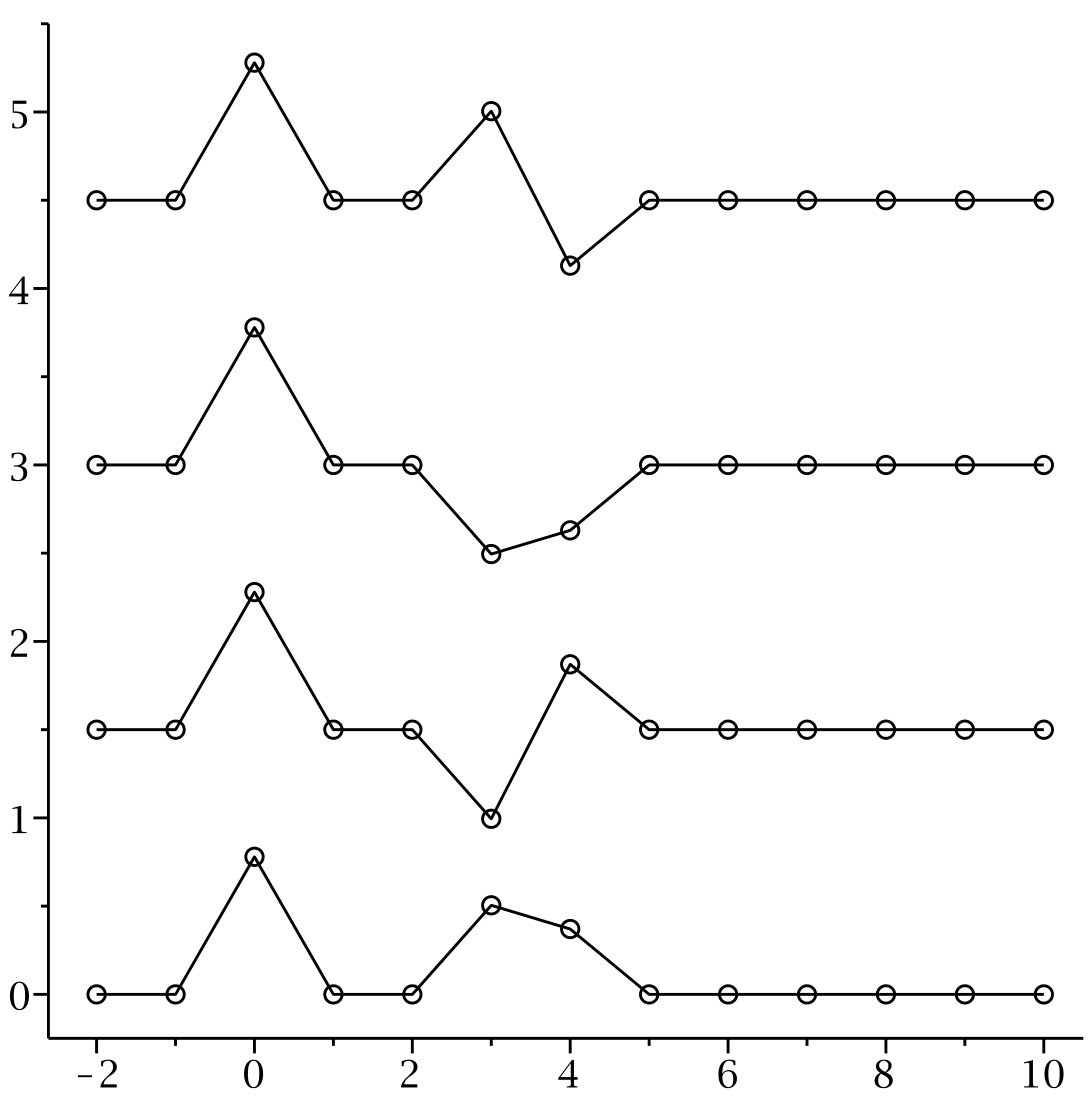 Figure 1
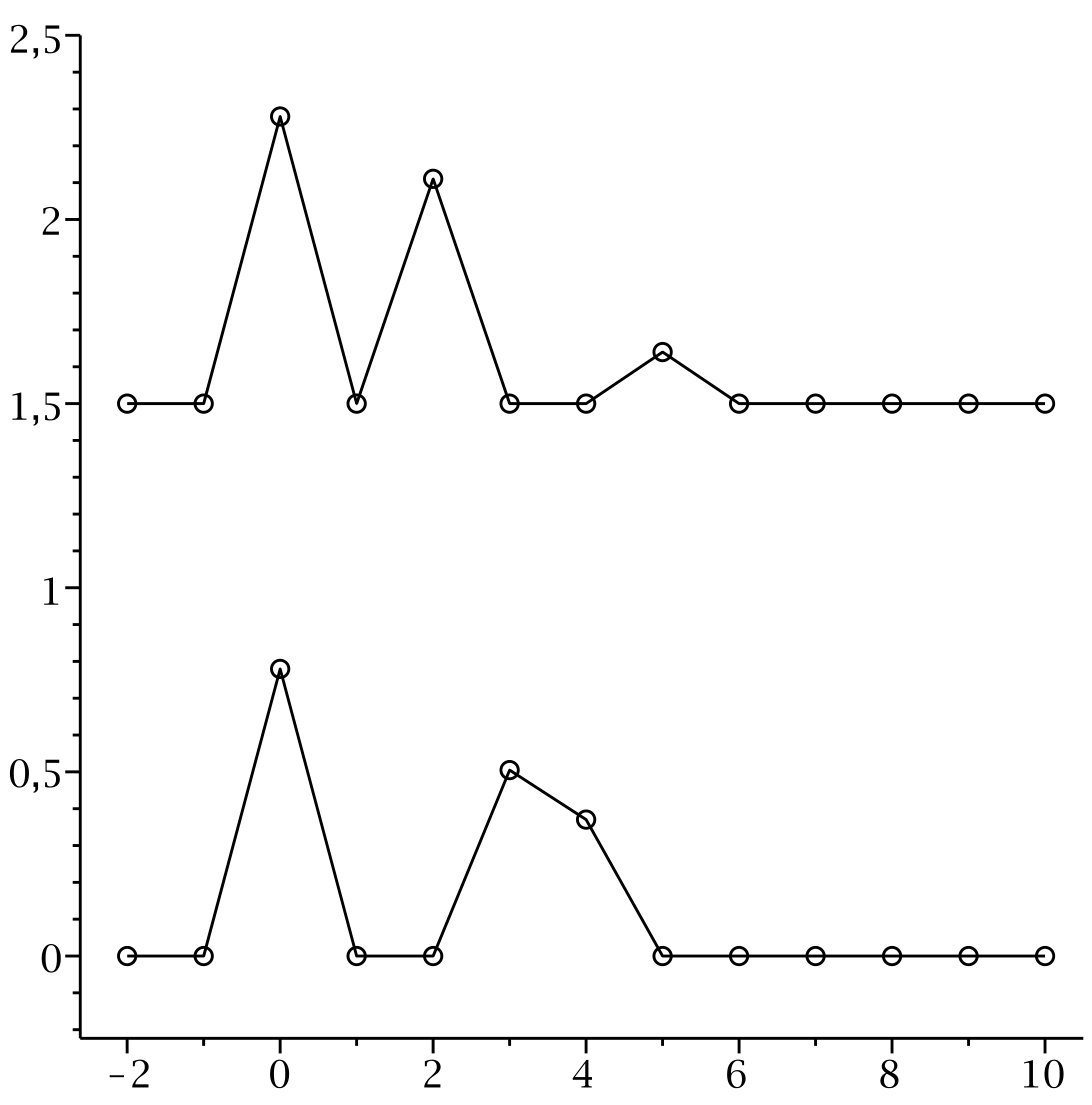 Figure 2
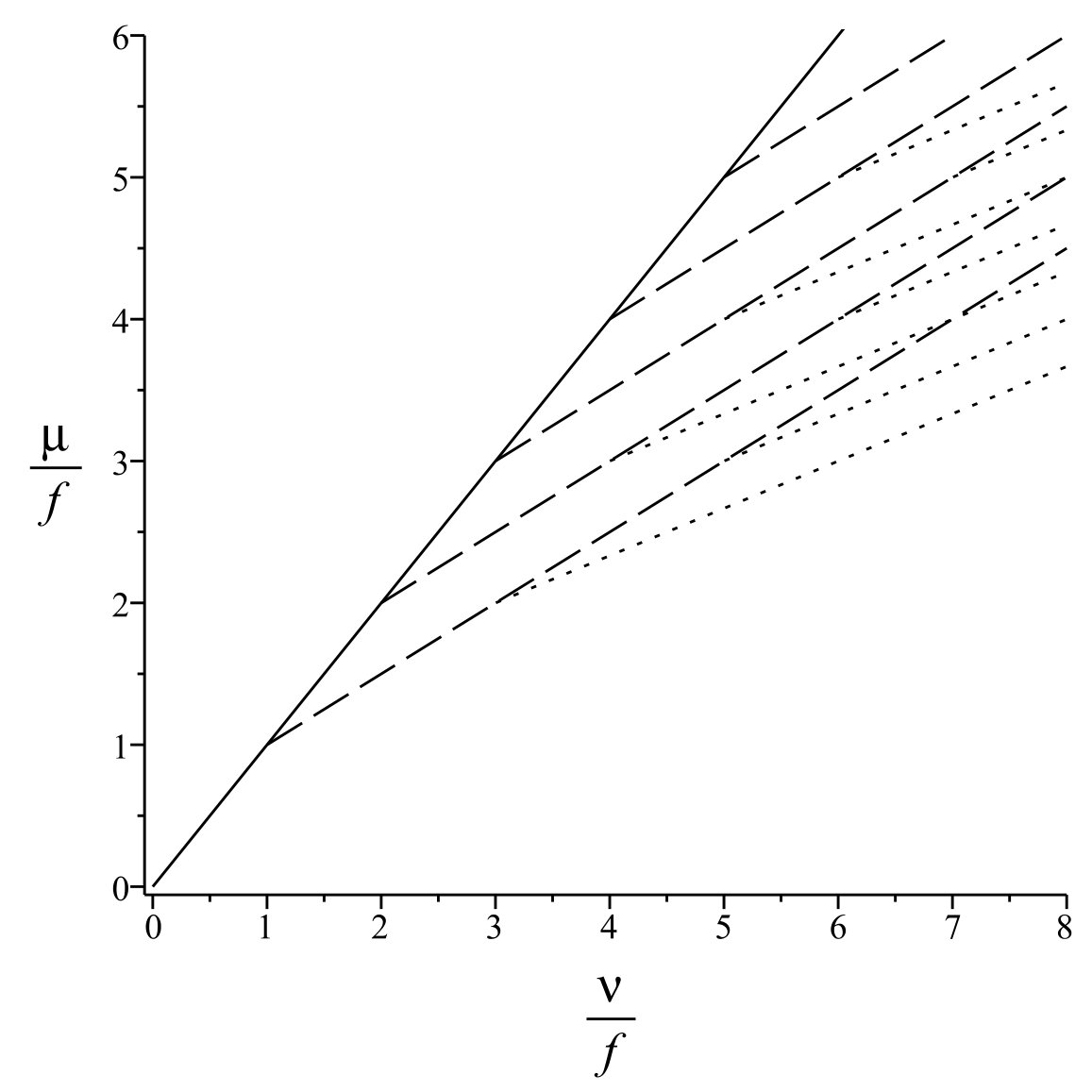 Figure 3
Peer Reviews
No public reviews on file for this paper yet. If you reviewed it on a platform where reviews are public (OpenReview, ICLR, NeurIPS, ICML), you can paste yours below so the community can read it here.
Videos
No videos yet. Explain this paper in a talk, walkthrough, or lecture? Add one.
Taxonomy
TopicsQuantum chaos and dynamical systems · Nonlinear Photonic Systems · Nonlinear Dynamics and Pattern Formation
Nonlinear Stark-Wannier equation
Andrea SACCHETTI
Department of Physics, Informatics and Mathematics, University of Modena e Reggio Emilia, Modena, Italy.
Abstract.
In this paper we consider stationary solutions to the nonlinear one-dimensional Schrödinger equation with a periodic potential and a Stark-type perturbation. In the limit of large periodic potential the Stark-Wannier ladders of the linear equation become a dense energy spectrum because a cascade of bifurcations of stationary solutions occurs when the ratio between the effective nonlinearity strength and the tilt of the external field increases.
Ams classification (MSC 2010): 35Q55, 81Qxx, 81T25.
This paper is partially supported by GNFM-INdAM. I deeply thank R. Fukuizumi for useful discussions about nonlinear Schrödinger equations.
1. Introduction
The dynamics of a quantum particle in a periodic potential under an homogeneous external field is one of the most important problems in solid-state physics and, more recently, in the theory of Bose Einstein Condensates (BECs). Because of the periodicity of the potential, it is expected the existence of families of stationary (metastable) states with associated energies displaced on regular ladders, the so-called Stark-Wannier ladders [15, 17, 27], and the wavefunction would perform Bloch oscillations.
Quantum dynamics becomes more interesting when we take into account the interaction among particles. In fact, in the framework of BECs accelerated ultracold atoms moving in an optical lattice [4, 5, 22, 26, 29] has opened the field to multiple applications, as well as the measurement of the value of the gravity acceleration using ultracold Strontium atoms confined in a vertical optical lattice [11, 21], direct measurement of the universal Newton gravitation constant [24] and of the gravity-field curvature [25].
Motivated by such physical applications we study, as a model for a confined accelerated BECs in a periodic optical lattice under the effect of the gravitational force, the nonlinear one-dimensional time-dependent Schrödinger equation with a cubic nonlinearity, a periodic potential and an accelerating Stark-type potential
[TABLE]
in the limit of large periodic potential, i.e. ; that is equation (1) is the so called Gross-Pitaevskii equation. Here, is the Planck’s constant, is the mass of the atom and is the strength of the nonlinearity term; the real valued parameters , , and are assumed to be fixed. In particular is a Stark-type potential with strength , that is it is locally a linear function: for any belonging to a fixed interval large enough.
We name equation (1) nonlinear Wannier-Stark equation. The well-known Wannier-Stark equation, where , has been extensively studied since the papers by Bloch [3] and Zener [37]. Assuming that the periodic potential is regular enough, then the spectrum of the associated operator covers the whole real axis. On the other side, if we neglect the coupling term between different bands, then it turns out that the spectrum of such a decoupled band approximation consists of a sequence on infinite ladders of real eigenvalues [30, 31]. The crucial point is to understand what happen to these eigenvalues when we restore the interband coupling term [32, 35, 36]. This question has been largely debated and it has been proved that these ladders of real eigenvalues will turn into ladders of quantum resonances, the so-called Wannier-Stark resonances (see [27] and the references therein). Analysis of the nonlinear Wannier-Stark equation, where , is a completely open problem and it is motivated by recent experiments of BECs in accelerating optical lattices.
By means of a simple recasting we swap the limit of large potential to a semiclassical equation (see eq. (3) below) where the strength of the Stark-type potential and the nonlinearity strength will depend on a semiclassical parameter . In the semiclassical limit of we will show that the time-independent nonlinear Schrödinger equation may be approximated by means of a discrete time-independent nonlinear Schrödinger equation which stationary solutions may be explicitly calculated. In particular, a cascade of bifurcations occurs when the ratio between the nonlinearity strength and the strength of the Stark-type potential increases; in the opposite situation, that is when this ratio goes to zero, we recover a local Wannier-Stark ladders picture.
Existence and computation of stationary solutions to equation (1) has been already considered by [13, 19, 20] when ; in these papers the authors reduce the problem of the existence and calculation of stationary solutions to the one related to a discrete nonlinear Schrödinger equation. In this latter problem has been observed by [2] that stationary solutions may bifurcate when some parameters of the model assume critical values. Here, we extend such analysis to the case where an external Stark-type potential is present, that is when . To this end we must introduce some technical assumptions on , that is must be a locally linear bounded function with compact support; in fact in the case of a true Stark potential where some basic estimates useful in our analysis don’t work because is not a bounded operator. Some results, like the occurrence of a cascade of bifurcations for the discrete nonlinear Schrödinger equation in the anticontinuous limit has been already announced in a physics-oriented paper [28] without mathematical details. We should also mention a recent paper [14] where bifurcations are observed in rotating Bose-Einstein condensates.
The paper is organized as follows: in §2 we introduce the model and we state our assumptions; in §3 we recall some technical results obtained by [13]; in §4 we derive the discrete nonlinear Schrödinger Wannier-Stark equation; in §5 we compute the finite-mode stationary solutions of the discrete nonlinear Schrödinger Wannier-Stark equation in the anticontinuous limit, it turns out that a bifurcation tree picture occurs; in §6 we prove the stability of these stationary solutions when we recover the discrete nonlinear Schrödinger Wannier-Stark equation; finally, in §7-8 we prove that stationary solutions to the complete equation (6) can be approximated by means of the finite-mode solutions derived in §5.
Notation
By we denote the space of vectors such that are real valued. Similarly,
[TABLE]
Let and two vectors belonging to a normed space with norm , and depending on the semiclassical parameter . By the notation , as , we mean that for any there exist a positive constant (independent of ) such that
[TABLE]
for some . By the notation , as , we mean that for some . By the notation , as , we mean that there exists and a positive constant independent of such that for any .
By we denote a generic positive constant independent of whose value may change from line to line.
2. Description of the model and assumptions
Here we consider the nonlinear Schrödinger equation (1) where the following assumptions hold true.
Hyp.1 * is a smooth, real-valued, periodic and non negative function with period , i.e.*
[TABLE]
and with minimum point such that
[TABLE]
For argument’s sake we assume that and .
In the following let us denote by .
Remark 1**.**
In physical experiments [11, 21] on accelerated BECs in optical lattices the periodic potential has the form for some ; hence has a unique minimum point in the interval . However, we could, in principle, adapt our treatment to a more general case where has more than one absolute minimum point in such interval.
Hyp.2 * is a smooth real-valued function such that*
[TABLE]
for some . Furthermore has compact support
Remark 2**.**
We require that is a bounded function with compact support for technical reasons; indeed, this assumption will play a crucial role in order to prove the results given in §6, 7, 8. However, in practical experiments [11, 21] on accelerated BECs in optical lattices it is expected that BECs perform Bloch oscillations in a finite region; hence, a model where the external field has a compact support and it is locally linear in the finite region where Bloch oscillations occur would fit the physical device.
By recasting
[TABLE]
then the above equation takes the form
[TABLE]
and the limit of large periodic potential is equivalent to the semiclassical limit where
[TABLE]
We recall here some results by [7, 8, 9] concerning the solution to the time-dependent nonlinear Schrödinger equation (3). Let be the Bloch operator formally defined on as
[TABLE]
For any , , the linear operator , formally defined as
[TABLE]
on the Hilbert space , admits a self-adjoint extension, still denoted by . The following estimate hold true (see Proposition 2.1 by [9]): let be an admissible pair with . Let , then there exists such that
[TABLE]
In order to discuss the local and global existence of solutions to (3) [9] introduced the following set in a more general situation where the potential is not bounded
[TABLE]
Then (see Theorem 4.2 by [9]), if there exists a unique solution to (3) with initial datum , such that
[TABLE]
for some depending on . We must underline that in our case because and are bounded functions.
In fact, this solution is global in time for any because , where is the spatial dimension, and (3) enjoys the conservation of the mass
[TABLE]
and of the energy
[TABLE]
where
[TABLE]
We may remark that such results hold true even when the Stark-type potential is replaced by an actual Stark potential, i.e. . In such a case .
Here, we look for stationary solutions to equation (3) of the form
[TABLE]
for some energy and wave function . Hence, equation (3) takes the form
[TABLE]
Remark 3**.**
We must underline that when a stationary solution to equation (6) is regular enough then is, up to a phase factor, a real-valued function (see Lemma 3.7 by [18] adapted to (6)). Hence, equation (6) can be replaced by the following equation
[TABLE]
where is real-valued.
Our aim is to look for real-valued stationary solutions to (7) with associated energy .
Remark 4**.**
Let be the translation operator. Since and then the stationary solutions to (7) when is a Stark potential, i.e. , have associated energies displaced on regular ladders; that is, if is a solution to (7) associated with , then is a solution to the same equation associated with . From this fact we expect that, under some circumstances, the dominant term of the energies associated to stationary solutions to (7) are displaced on ladders for some range of values of , even when is a Stark-type potential satisfying Hyp.2.
3. Preliminary results. Bloch functions in the semiclassical limit
3.1. Bloch Decomposition and Wannier functions
Here, we briefly resume some known results by [6, 23] concerning the spectral properties of the self-adjoint realization, still denoted by , of the Bloch operator formally defined on as (5). Its spectrum is given by bands. Let , where and is the period of the periodic potential , be the Brillouin zone, the elements of the Brillouin zone are denoted by and they are usually named quasi-momentum (or crystal momentum) variable.
Let denote the Bloch functions associated to the band functions , . Here, we collect some basic properties about the Bloch and band functions. The band and Bloch functions satisfy to the following eigenvalues problem
[TABLE]
with quasi-periodic boundary conditions
[TABLE]
The Bloch functions may be written as
[TABLE]
where is a periodic function with respect to : . For any fixed the spectral problem (8) has a sequence of real eigenvalues
[TABLE]
such that . As functions on , both Bloch and band functions are periodic with respect to :
[TABLE]
and they satisfy to the following properties for any real-valued :
[TABLE]
Furthermore, if is an even potential, i.e. , then , are even functions while are odd functions. The band functions are monotone increasing (resp. decreasing) functions for any if the index is an odd (resp. even) natural number. The spectrum of is purely absolutely continuous and it is given by bands:
[TABLE]
In particular we have that
[TABLE]
The intervals are named gaps; a gap may be empty, that is , or not. It is well known that, in the case of one-dimensional crystals, all the gaps are empty if, and only if, the periodic potential is a constant function. Because we assume that the periodic potential is not a constant function then one gap, at least, is not empty. In particular when is small enough then we have that the following asymptotic behavior [16, 33, 34]
[TABLE]
holds true for some ; hence,the first gap between and is not empty in the semiclassical limit. Furthermore, the first band turns out to be exponentially small, i.e.
[TABLE]
in (14) we will give an expression for such a constant .
The Bloch functions are assumed to be normalized to on the interval :
[TABLE]
where when and when (see Eq. (4.1.8) by [6]). Furthermore, the Bloch functions are such that (see Eq. (4.1.6a) by [6])
[TABLE]
and (see Eq. (4.1.10) by [6])
[TABLE]
where denotes the Dirac’s . From the Bloch decomposition formula it follows that any vector can be written as (see Eq. (5.1.5) by [6] or Theorem XIII.98 by [23])
[TABLE]
The family of functions is called the crystal momentum representation of the wave function and it is defined as
[TABLE]
By construction any function is a periodic function and the transformation
[TABLE]
is unitary:
[TABLE]
Let be the basic Wannier function associated to the -th band, that is
[TABLE]
We define a family of Wannier functions as
[TABLE]
Basically, in the semiclassical limit of small, the Wannier function is localized on the -th well, that is in a neighborhood of . The following properties hold true
[TABLE]
and we have the following relation between the Wannier and the Bloch functions:
[TABLE]
If we set
[TABLE]
then we may represent a wave function as
[TABLE]
Such a transformation is unitary
[TABLE]
with inverse
[TABLE]
Remark 5**.**
The standard “tight binding” model is obtained by substituting (13) in (3), and it reduces (3) to a discrete nonlinear Schrödinger equation. In fact, in order to improve the estimate of the remainder terms of the discrete nonlinear Schrödinger equation we decompose the wave function on a different base where the vectors of such a base are obtained by means of the single well semiclassical approximation described in §3.2.
3.2. Semiclassical construction
Here we restrict our attention to just one band, say the first one . By assuming small enough then the gap between the first band and the remainder of the spectrum is open, see equation (10). Let be the spectral projection of on the first band; by [10] we can find a “good” orthonormal basis of .
In one dimension let
[TABLE]
be the Agmon distance between and (associated to the energy level corresponding to the minimum value of the potential ) and let
[TABLE]
be the Agmon distance between two adjacent wells; by periodicity of the potential then is independent of the index .
Here we summarize some important properties of (see [10] and Appendix A by [13]). Let be the “single well potential” obtained by filling all the well, but one; that is where is a smooth and non negative function such that in a small neighborhood of and for any for some and is fixed. Then the operator has discrete spectrum in the interval and we call such eigenvalues single well states. We denote by the first one, the so called “single well ground state”, and by the associated eigenvector.
Remark 6**.**
By means of semiclassical arguments it follows that [16, 33, 34]
[TABLE]
Furthermore,
[TABLE]
for some .
If we denote then the family is a family of linearly independent vectors localized on the th well. Then, taking their projection on and orthonormalizing the obtained family we finally get the base of .
Lemma 1**.**
The vectors of the orthonormal base of are such that:
- i.
The matrix with real-valued elements can be written as
[TABLE]
where is the tridiagonal Toeplitz matrix, i.e.,
[TABLE]
* is such that for any then*
[TABLE]
for some positive constant , and the remainder term is a bounded linear operator from to with bound
[TABLE]
for some positive constant independent of and , and for some positive constant which depends only on .
- ii.
Let be the translation operator , where is the period of . Then, .
- iii.
All the functions can be chosen to be real-valued by means of a suitable gauge choice.
- iv.
For any and for some positive constant independent on the indexes and , we have that
[TABLE]
- v.
There exists a constant independent of such that
[TABLE]
- vi.
For any , , and where the constants are independent of and .
4. Construction of the discrete nonlinear Stark-Wannier equation
Let the projection operator associated to the first band of (see §3.1) and let . Let
[TABLE]
By the Carlsson’s construction resumed in §3.2 we may write by means of a linear combination of a suitable orthonormal base of the space , that is
[TABLE]
where and
[TABLE]
because , and then , is a real-valued function by Remark 3 and are real valued too since Lemma 1.iii. In fact, when we make use of the fixed point argument in §7 and when we prove the existence result of stationary solutions in §8 we work with vectors ; then in the sequence we may assume that for any .
Remark 7**.**
By construction
[TABLE]
Remark 8**.**
We must underline that the standard tight-binding model is constructed by making use of the Wannier functions (see (13)) instead of (18) and (19). In fact, the decomposition (13) turns out to be more natural and it has the advantage to work for any range of ; decompositions (18) and (19) are more powerful than (13) in the semiclassical regime of and they have the great advantage that the vectors are explicitly constructed by means of the semiclassical approximation (see Lemma 1).
By inserting (18) and (19) in equation (7) then it takes the form
[TABLE]
where and are such that
[TABLE]
The following result immediately follows by Lemma 1.
Lemma 2**.**
We have that
[TABLE]
where satisfies (16) and
[TABLE]
where is defined by Lemma 1.i and it satisfies to the following estimate for some : let and , then
[TABLE]
for some positive constant .
Let be the Agmon distance between two points and let , , be the Agmon distance between the bottoms and of two adjacent wells of the periodic potential (for further details see §3.2); by periodicity does not depend on the index .
Lemma 3**.**
We have that
[TABLE]
where for any there exists such that
[TABLE]
and there exists such that
[TABLE]
Furthermore, for any because is bounded, and
[TABLE]
where is a bounded function such that
[TABLE]
where are such that and ; by construction .
Proof.
By inserting (18) and (19) in one gets
[TABLE]
Now, we set
[TABLE]
Estimates of and directly come from the properties collected in Lemma 1. Indeed
[TABLE]
for any and some , because is bounded; hence the estimate
[TABLE]
follows. Similarly,
[TABLE]
where is the characteristic function and where is the compact support of . Concerning estimate (23) we consider the term when ; let
[TABLE]
where
[TABLE]
because , Lemma 1.ii and Lemmata 4.iii and 7 by [13]. More precisely, let then
[TABLE]
where is the characteristic function on . Then (the properties below concerning are given in Lemma 4.iii by [13], where is the single well ground state defined in §3.2)
[TABLE]
Hence,
[TABLE]
Concerning the estimate of the remainder terms we have that
[TABLE]
because is bounded and by making use of the same arguments as before. Similarly we get the same estimate for . ∎
Remark 9**.**
By construction and since is normalized to one it follows that for some positive constant independent of .
Finally, concerning the nonlinear term we recall the following result which follows by [13] (where we choose , for the purpose of completeness the detailed proof is given in a separate appendix).
Lemma 4**.**
We have that
[TABLE]
where
[TABLE]
and
[TABLE]
satisfies to the following estimate: let , then for any there exists such that
[TABLE]
Remark 10**.**
By Lemma 1.vi it follows that as goes to zero.
Therefore, equation (22) takes the form
[TABLE]
where
[TABLE]
Definition 1**.**
We define the discrete nonlinear Stark-Wannier equation (hereafter DNLSWE) as
[TABLE]
where .
As already explained in Remark 2 we expect that the solutions to equation (28) are displaced, when (corresponding to the case ), on regular ladders, that is the solutions are of the form for some and any . We will call, hereafter, the value as the -th rung of the ladder connected to . In the case that is a linear function on an interval , according with Hyp. 2, then we will see that the structure of the ladder locally occurs, so even in such a case we may speak of rungs of such a kind of ladders of stationary solutions.
5. Anticontinuous limit of the DNLSWE
Let us set
[TABLE]
where
[TABLE]
since Remark 10 and Lemma 1.i. For argument’s sake, we assume that . Hence (28) takes the form
[TABLE]
and in the anticontinuous limit then (31) becomes
[TABLE]
5.1. Finite-mode solutions to the anticontinuous limit equation (32)
Here, we look for stationary solutions to (32) under the normalization condition
[TABLE]
Definition 2**.**
We say that the anticontinuous limit equation (32), under the normalization condition , has a one-mode solution if there exists a set , hereafter called solution-set, with finite cardinality, a real value and a normalized vector where and solve
[TABLE]
and where if . The real value is hereafter called the “energy” associated to the stationary solution .
When then we simple recover a (kind of) Stark-Wannier ladder, that is the solution-sets are given by simple sets of the form for any and we have a family of admitted “energies” with associated stationary solutions . In fact, it is an exact Stark-Wannier ladder when .
Assume now that the effective nonlinearity strength is not zero, that is for argument’s sake. In such a case, equation (33) has finite mode solutions , associated to sets with finite cardinality , given by
[TABLE]
with the condition
[TABLE]
because we have assumed that and . The normalization condition reads
[TABLE]
In the case then again for any and (38) reduces to
[TABLE]
where condition (37) holds true because we have assumed that ; the associated stationary solution takes the form:
[TABLE]
That is we recover a kind of (perturbed) Stark-Wannier ladder.
Remark 11**.**
From this fact we can conclude that the anticontinuous limit (32) always admits a ladder-type family of normalized one-mode solutions.
5.2. Finite-mode solutions to equation (33) associated to solution-sets with finite cardinality bigger that 1
In order to look for finite-mode solutions with the normalization condition (38) implies that
[TABLE]
5.2.1. Existence of finite-mode solutions.
Stationary solutions associated to the energy (40) are given by
[TABLE]
In the case let with . The eigenvalue equation (40) becomes
[TABLE]
where condition becomes
[TABLE]
that is
[TABLE]
In conclusion, if
then (45) is not satisfied and there are no stationary solutions associated to solution-sets of the form with cardinality ;
- -
we have a family of two-mode solutions associated to solution-sets with given by (44) and where
[TABLE]
Finally, we can extend such an argument to any integer number obtained the following result.
Theorem 1**.**
Let , with and positive integer numbers such that
[TABLE]
Then is a solution-set connected to the -th rung of a (kind of) Stark-Wannier ladder and equation (33) has a -mode solution with
[TABLE]
and associated normalized stationary solution given by (43).
Remark 12**.**
We should underline that some of such a solution may be associated to the same “energy” . For instance let and let us consider the sets and . Recalling that is a linear function in both sets and then they are associated to the same value (where we assume, for argument sake, that and ) of energy
[TABLE]
In Figure 1 - left panel - we plot the 4 solutions (43) corresponding to the set . In Figure 1 - right panel - we plot the solutions (43) with sign , corresponding to the sets and .
Remark 13**.**
If the solution-set then , , is linear and thus we locally recover a Stark-Wannier ladder structure. That is is a solution-set too, provided that , and . We will say that is connected with the [math]-th rung of the ladder, and that is connected with the -th rung of the ladder.
Remark 14**.**
In the limit of small enough then since Remark 10 and (30); therefore the stationary solutions takes the value if and if , and the energy belongs to an interval with center , for some , and with amplitude of order .
5.2.2. Bifurcation of stationary solutions
We consider solution-sets associated to a given rung of the (kind of) Stark-Wannier ladder satisfying the condition where is a linear function. That is we consider energies in the interval . We can see that stationary solutions to equation (33) associated to such solution-sets may bifurcate when the ratio is a positive integer number.
In order to count how many stationary solutions we have let us introduce the following function (see Abramowitz and Stegun [1], p. 825).
Definition 3**.**
Let , , be the number of ways of writing the integer number as a sum of positive integers without regard to order, with the constraint that all integers in a given partition are distinct.
E.g.: , , and .
Theorem 2**.**
When takes the value of a positive integer number then stationary solutions to (33), associated to solution-set , bifurcate. Furthermore, the total number of solutions-sets associated to a given rung of the (kind of) Wannier-Stark ladder, assuming that all these sets are contained in the interval , is given by
[TABLE]
Proof.
First of all, because the stationary problem (33) is translation invariant and , provided that the solution-sets are contained in the interval , then we can always restrict ourselves to the [math]-th rung of the ladder such that , that is the solution-set has the form with positive and integer numbers. Hence, (40) becomes
[TABLE]
and condition (37) implies the following condition on the solution-set
[TABLE]
where
[TABLE]
Let be the collection of sets satisfying (50), and let be the collection of sets of all non negative integer numbers, including the number [math], which sum is equal to , without regard to order with the constraint that all integers in a given partition are distinct; e.g. , and . Hence, by construction
[TABLE]
In conclusion, we have shown that the counting function defined as the number of solution-sets of integer numbers satisfying the conditions (50) and such that , is given by
[TABLE]
Theorem 2 is so proved. ∎
Remark 15**.**
A cascade of bifurcation points, when takes the value of any positive integer, occurs; indeed, when the ratio becomes larger than a positive integer then new stationary solutions appear. This fact can be seen in Figure 2, where we plot the values of , when belongs to the interval , associated to solution-sets such that , that is we plot the value of energies associated to the [math]-th rung of the (kind of) Wannier-Stark ladder. By translation , , and thus this picture occurs for each rung of the ladder and then the collection of values of associated to stationary solutions is going to densely cover intervals of the real axis.
Remark 16**.**
One can see that grows quite fast, indeed the following asymptotic behavior holds true [1]:
[TABLE]
Hence
[TABLE]
as goes to infinity, where is the imaginary error function. In particular, because (see Remark 14) , then we have that the energy lies in an interval with center at and amplitude of order , and the number of stationary solutions is of order
[TABLE]
for some positive constant . That is the energy spectrum densely fill the interval when goes to zero.
Remark 17**.**
Since we assumed that the parameters , , and are fixed and that then the rescaling (2) immediately implies that the effective nonlinear coupling strength parameter is of order , where plays the role of a semiclassical parameter. Hence, the bifurcation parameter is such that
[TABLE]
and we have a dense energy spectrum. One can also consider the case where the parameters depend on ; a similar approach has been used, e.g., by [12]. If the nonlinear coupling strength parameter depends on some power by then for some power and
[TABLE]
If then we have a dense energy spectrum as in the case above; if then we have a single Stark-Wannier ladder; if then we observe the bifurcation phenomenon.
5.2.3. When do -mode stationary solutions arise from -mode stationary solutions?
If one looks with more detail the bifurcation cascade one can see that we have -mode solutions for any value of , provided that for some large enough. Let us restrict our analysis, for sake of simplicity, to solution-sets contained in the interval where is a linear function.
As said above, -mode stationary solutions are associated to solution-sets of the form
[TABLE]
under condition (37). Now, let us consider, as a particular family of -mode solutions, solution-sets of the form (51) for any and , assuming that . They are associated to
[TABLE]
and then condition (37) implies that
[TABLE]
Hence, we can observe a second bifurcation phenomenon: stationary solutions associated to solution-sets with elements arise from stationary solutions associated to solution-sets with elements when becomes bigger than the critical value .
We can summarize such a result as follows
Theorem 3**.**
If then stationary solutions to (32), associated to solution-sets , are localized on a number of sites less than , at a stationary solution localized on sites bifurcates and a new stationary solution localized on sites arises.
6. Existence of solutions to the DNLSWE
Let and b a finite-mode solution to (32) associated to a solution-set given by Theorem 1. Now, we will prove, by a stability argument, that this solution becomes a solution to (31) when is small enough. To this end we have to remind that goes to zero when goes to zero according with Lemma 1.i.
Theorem 4**.**
Let . Let be a solution-set to (32) with associated energy and normalized stationary solution given by (36). We assume that . Then, if is small enough there exists a stationary solution to the DNLSWE (31) associated to and such that
[TABLE]
Proof.
First of all let us recall that from Remark 14 then . In the following let us omit the upper letters in and for sake of simplicity. If we rescale and , and if we set and then equations (31) and (32) take the form
[TABLE]
with anticontinuous limit
[TABLE]
Therefore, any solution and to (31) is associated to a solution to (52), and all the solutions to (53) associated to the values given by Theorem 1 are isolated in by construction when there are no bifurcations, that is for .
Let be the map defined as
[TABLE]
We are going to look for solutions to equation ; where we already know that equation has solutions associated to the ones given by Theorem 1. We may extend the solutions to (53), obtained in the anticontinuous limit , to the solutions to equation (52) for small enough if the tridiagonal matrix
[TABLE]
obtained deriving the previous equation by , is not singular at , where takes the value of a solution to (43) obtained for . The linearized map can be written as , where
[TABLE]
Hence
[TABLE]
Lemma 5**.**
Let be small enough, then it follows that
[TABLE]
Proof.
Assume at first that . In this case for any such that and
[TABLE]
as goes to zero, because of Lemma 3. Hence
[TABLE]
Recalling now that and then . Similarly, we can easily extend such arguments to any integer number . In this case , for and such that , , . Then
[TABLE]
hence
[TABLE]
The proof of the Lemma is so completed.
∎
Now we are ready to conclude the proof of Theorem 4. Indeed, by Lemma 5, the linearized map is invertible with inverse uniformly bounded. Therefore, by the Implicit Function Theorem, there exists a neighborhood of [math] such that if belongs to such a neighborhood then there exists a unique solution to equation in a -neighborhood of , where is an isolated solution to because bifurcations occur at . Since , for any small enough, then for any for some . From this fact and because the map is then we can conclude that when is small enough then there exists a solution to equation such that
[TABLE]
By construction it follows also that when then
[TABLE]
hence
[TABLE]
from (58). Then the proof of the Theorem is given. ∎
Remark 18**.**
Since we can always normalize to by means of suitable rescaling of the nonlinearity parameter we can conclude that is a normalized solution to (31) associated to for some . Furthermore, by construction (see §3.2), the map is when we are far form the bifurcation points ; then we can conclude that for any fixed and such that then equation (31) has a solution and where is normalized and it satisfies (58) and .
7. Fixed point argument
Here, we go back to equation (22) and, at first, we justify the existence of by means of a fixed point argument. Recalling that and where and where , then the value of corresponding to is such that . Hence, we consider the second equation of (22) for in a neighborhood of with width of order .
Theorem 5**.**
Let , , where and , let small enough. Let be any fixed real and positive number, then for any , with , there exists a unique smooth map
[TABLE]
such that is a solution to the second equation of (22) for small . Moreover, is small as in the sense that there exists a positive constant , dependent on and independent of , such that
[TABLE]
Proof.
We make use here of same ideas already developed by [13] adapted to the case of a tilted periodic potential. Let be defined as in §3.2 and let be fixed. Note that the operator on has inverse operator for sufficiently small provided that
[TABLE]
and thanks to the fact that the , that is a bounded operator, and that from (4). Precisely, there exists a constant independent of such that
[TABLE]
Then the second equation of (22) may be written as
[TABLE]
where is fixed and where we set , and
[TABLE]
We are going to show that is a contraction map in
[TABLE]
for some . Indeed, let , and let and , we have
[TABLE]
since Remark 7 and (4). Then, by the Gagliardo-Nirenberg inequality, it follows that
[TABLE]
since , and because by Remark 7 and Lemma 1.vi
[TABLE]
Hence
[TABLE]
for some small enough. Furthermore
[TABLE]
hence
[TABLE]
where
[TABLE]
since
[TABLE]
Then there exists a unique solution to equation (60) for small . Moreover, by construction the solution is given by
[TABLE]
where and . Hence
[TABLE]
and thus
[TABLE]
for some positive constant . This fact completes the proof. ∎
We must underline that linearly depends on and thus the map is a smooth map. In particular the following result holds true.
Lemma 6**.**
Let be such that , where is any fixed and positive number. Then for any such that then there exists and it is such that
[TABLE]
Proof.
Indeed, equation (60) becomes
[TABLE]
where we set
[TABLE]
A straightforward computation gives that
[TABLE]
where
[TABLE]
and (62) reduces to
[TABLE]
The same arguments used in the proof of Theorem 5 yields to the following estimate
[TABLE]
because and (4). Then immediately follows. ∎
Remark 19**.**
From Lemma 6 it follows that the linear map satisfies the estimate
[TABLE]
8. Existence of stationary solutions
Theorem 6**.**
Let and let small enough. Let be a finite-mode normalized solution associated to a solution-set satisfying the assumption of Theorem 4. Then there exists a stationary solution to equation (26) such that
[TABLE]
Proof.
Let us omit, for the sake of simplicity, the upper letter . We have to consider the first equation of (26) where , and are defined by (29):
[TABLE]
where is defined by (27) and where the map
[TABLE]
is norm bounded by (see Lemma 2, Lemma 3, equation (30), Lemma 4 and Theorem 5)
[TABLE]
for some and for any , where is a positive constant and is a positive constant depending on .
Now, let us consider the following mapping
[TABLE]
defined as
[TABLE]
where and where is the solution to the second equation of (26) for small given by Theorem 5.
By construction, coincides with the discrete nonlinear Schrödinger equation DNLSWE (28), while coincides with equation (64).
Lemma 7**.**
* is a map in . In particular:*
- i.
for any fixed there exists a positive constant such that: he map satisfies
[TABLE]
- ii.
the maps and are linear maps such that
[TABLE]
- iii.
the map does not directly depend on and it is such that
[TABLE]
for any such that .
- iv.
the map satisfies
[TABLE]
In conclusion
[TABLE]
Proof.
Estimate (66) has been already proved (see estimate (37) by [13]). Concerning we recall that it is the linear map defined in Lemma 3, hence is independent of and such that (see Lemma 1.iv): , Similarly for as defined by (27). Concerning we recall that is is defined in Lemma 3 and it does not directly depend on , furthermore the estimate (67) on the -norm comes from the fact that linearly depends of and from Lemma 6. Concerning the term it is defined as ; then immediately follows that the map is smooth. Furthermore, a straightforward calculation yields to the following expression
[TABLE]
where we set . Since by Lemma 1.iv then the leading term in is given by
[TABLE]
From this fact and because (Theorem 5), (Remark 19), (Lemma 1.vi) and Lemma 1.v then it follows that the leading term in is estimated by
[TABLE]
By collecting all these facts and since (4) the the proof follows. ∎
Now, we fix , then
[TABLE]
Lemma 8**.**
Let and be a solution to equation , as given by Theorem 4; the linear map is one-to-one and onto.
Proof.
Again, let us omit the upper letter when this does not cause misunderstanding. By construction, the linear map
[TABLE]
is associated to a tridiagonal matrix defined as
[TABLE]
Here, we make use of the result given in Appendix A by [2]; in particular, because is exponentially small as goes to zero we only have to check that
[TABLE]
uniformly holds true with respect to , where is close to and is close to . Indeed, the left hand side of (71) turns out to be close to , where is given by (56) and, by Lemma 5, it is such that for any ; furthermore . From this fact and from the argument given in Appendix A by [2] then the linear map is one-to-one and onto. ∎
Now, we are ready to conclude the proof of Theorem 6. Le be the solution to (28) associated to the finite-mode solution satisfying the assumptions of Theorem 6. By the Implicit Function Theorem, there exist an -independent such that if then there exists a unique solution in a -neighborhood of satisfying . Then we can conclude that there exists such that for any there is a unique solution to , and it is such that
[TABLE]
since and (70). Then the Theorem follows where , and , furthermore
[TABLE]
because of Theorems 4, 5, equation (72) and Lemma 1.vi. Theorem 6 is so proved. ∎
Appendix A Proof of Lemma 4
Let us recall that satisfies to the following estimates (see (28) and (29) in [13])
[TABLE]
and
[TABLE]
Moreover, from Lemma 1, the following inequalities hold true:
[TABLE]
[TABLE]
[TABLE]
Furthermore, we recall also the following Sobolev inequality (see Theorem 8.8 in Brezis)
[TABLE]
Now, let
[TABLE]
where we set
[TABLE]
and
[TABLE]
By the proof of Lemma 3 in [13] we have that for any there exists such that the vector can be estimated as follows
[TABLE]
For what concerns the term we observe that
[TABLE]
where
[TABLE]
[TABLE]
[TABLE]
Therefore
[TABLE]
Hence,
[TABLE]
The reference list from the paper itself. Each links out to its DOI / PubMed record.
- 1[1] Abramowitz M., and Stegun I.A., Handbook of Mathematical Functions , National Bureau of Standards (1972).
- 2[2] Alfimov G.L., Brazhni V.A., and Konotop V.V., On classification of intrinsic localized modes for the discrete nonlinear Schrödinger equation , Phys. D: Nonlinear Phenomena 194 , (2004) 127.
- 3[3] Bloch F., Über die Quantenmechanik der Elektronen in Kristallgittern , Z. Phys. 52 (1928) 555
- 4[4] Bloch I., Ultracold quantum gases in optical lattices , Nature Phys., 1 , (2005) 23.
- 5[5] Bloch I., Quantum choerence and entanglement with ultracold atoms in optical lattices , Nature, 453 (2008) 1016.
- 6[6] Callaway J., Quantum Theory of the Solid State: Part A and B , (New York and London: Academic Press) (1974).
- 7[7] Carles R., On the Cauchy problem in Sobolev spaces for nonlinear Schrödinger equations with potential , Portugal Math. (N.S:) 65 (2008) 191.
- 8[8] Carles R., Nonlinear Schrödinger equation with time dependent potential , Commun. Math. Sci. 9 (2011) 937.