Cut and compute: Quick cascades with multiple amplitudes
Joydeep Chakrabortty, Anirban Kundu, Rinku Maji, Tripurari, Srivastava

TL;DR
This paper extends a previously proposed method for calculating decay widths in cascade decays to include multiple cascades and interference effects, providing a faster alternative with results matching standard Monte Carlo methods.
Contribution
The authors develop an extended algorithm for cascade decay calculations that handles multiple cascades and interference, broadening the method's applicability.
Findings
Algorithm shows excellent agreement with Monte Carlo simulations.
Efficient computation of complex decay chains with interference effects.
Applicable to both symmetric and asymmetric four-body decays.
Abstract
In an earlier paper we have proposed a novel method to compute the decay width for a general cascade decay where the propagators are off-shell and may be of different spins. Here, we extend our algorithm to accommodate those decays that are mediated by more than one such cascades. This generalizes our prescription and widens its applicability. We compute the three- and four-body toy decay chains where identical final states appear through different cascades. Here, we also provide the algorithm to calculate the interference terms. For four-body decays we discuss both symmetric and asymmetric cascades, providing the expressions for the detailed phase space structure in each case. We find that the results obtained with this algorithm have a very impressive agreement with those from standard softwares using a sophisticated Monte Carlo based phase space integration.
Click any figure to enlarge with its caption.
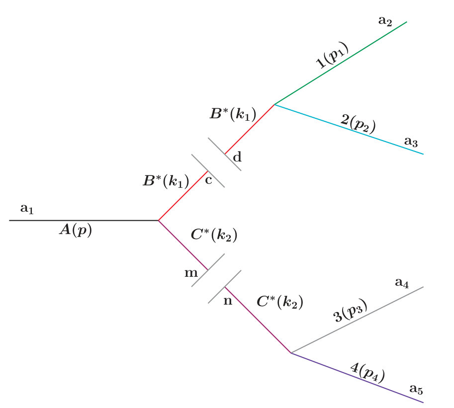 Figure 1
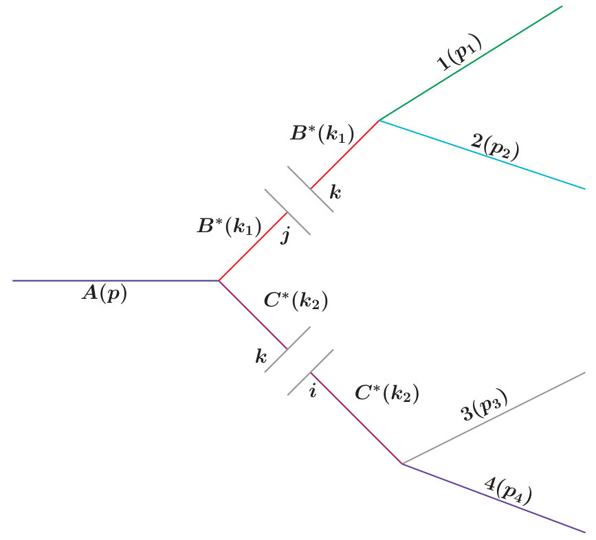 Figure 2
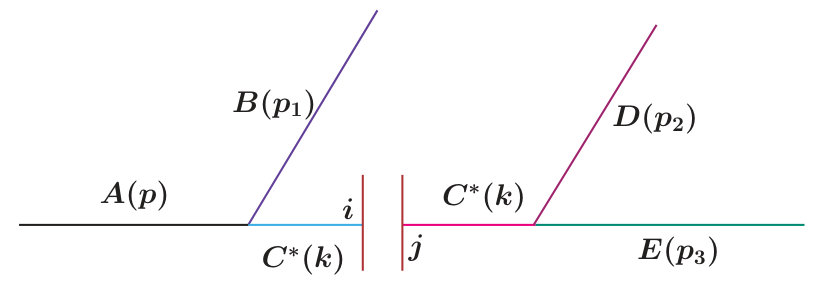 Figure 3
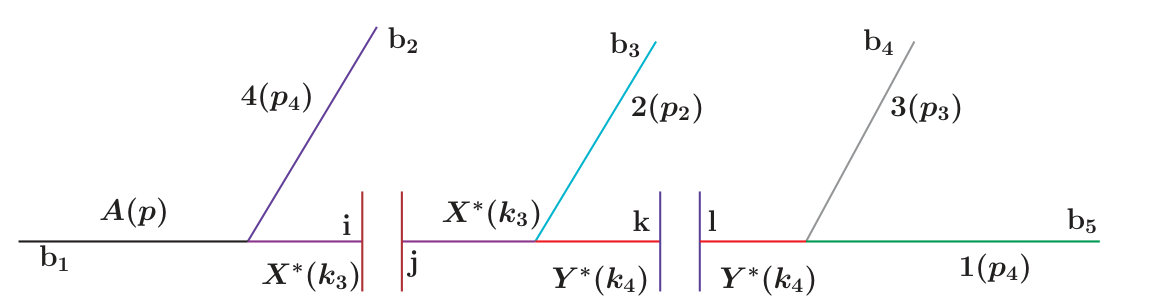 Figure 4
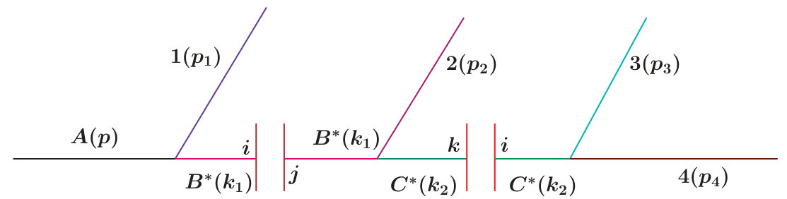 Figure 5
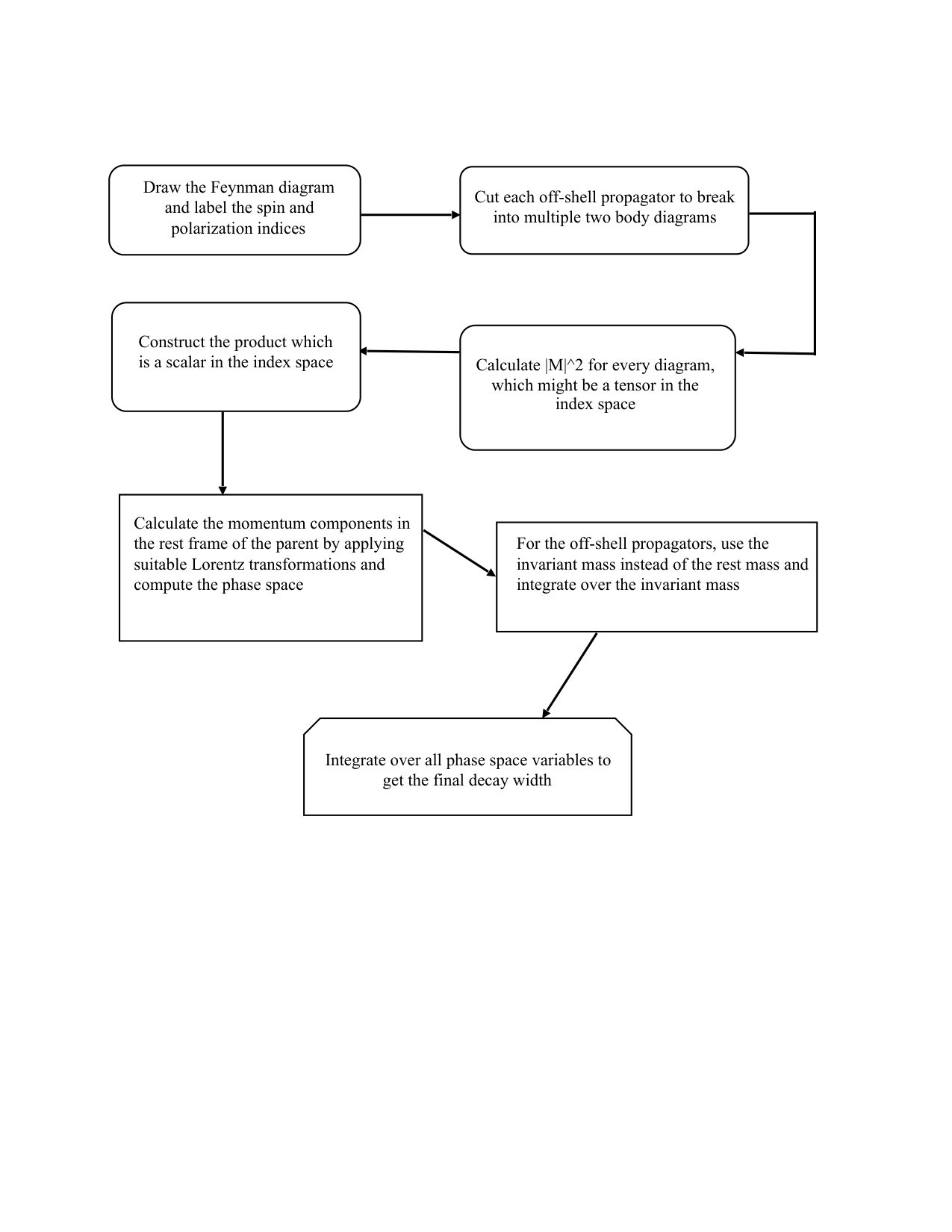 Figure 6
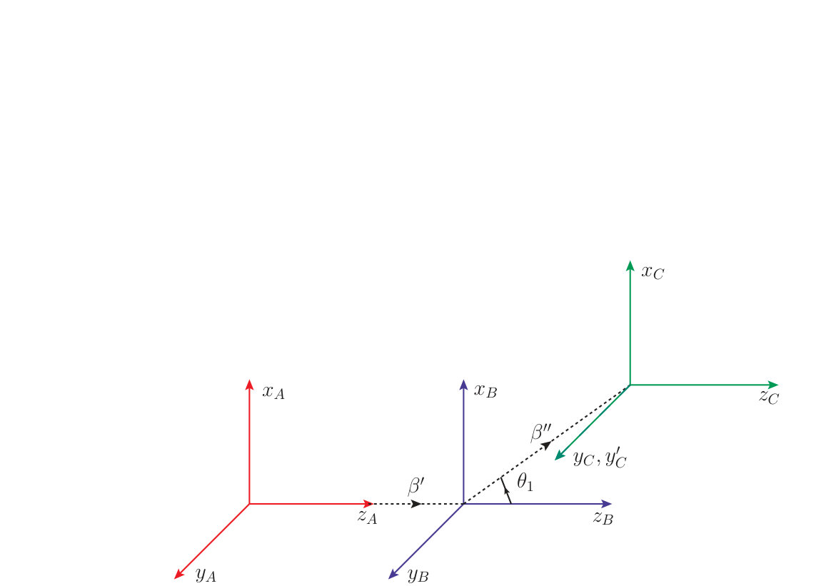 Figure 7
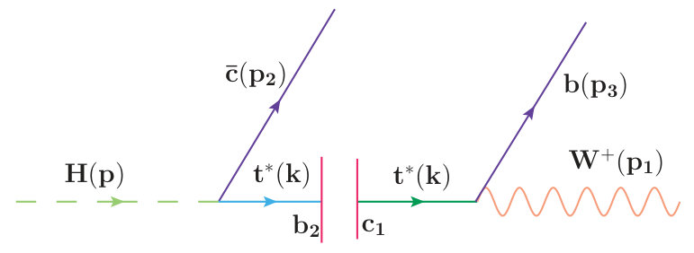 Figure 8
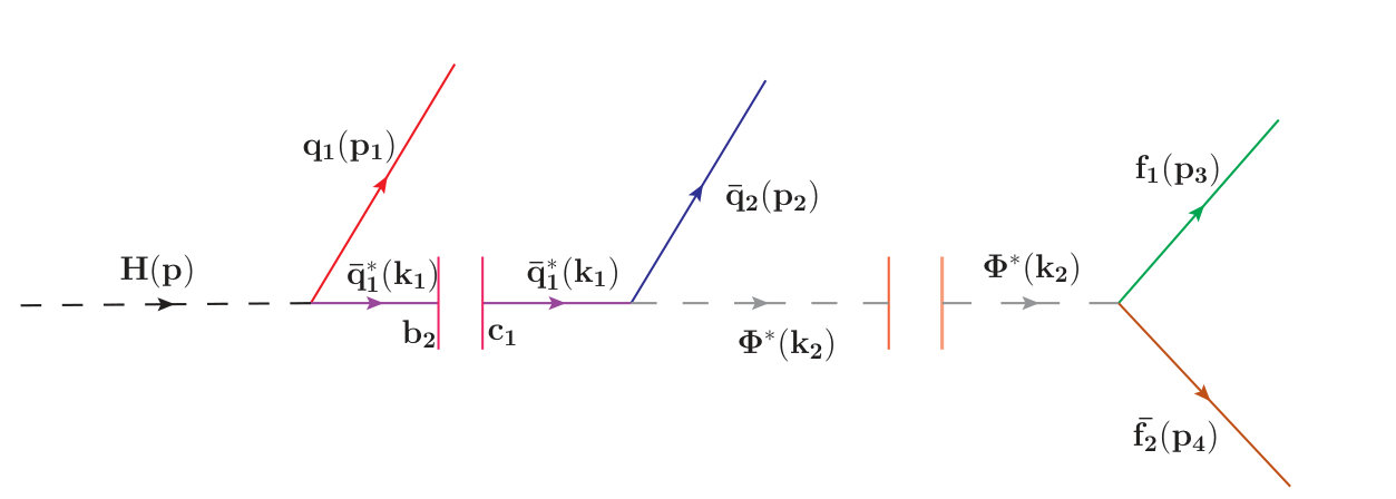 Figure 9
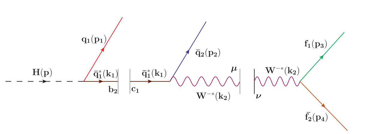 Figure 10
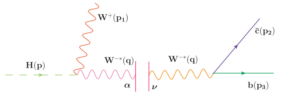 Figure 11
| (GeV) | (GeV) | (GeV) | (GeV) |
|---|---|---|---|
| (C1) | (C1) | (C1) | (C1) |
| (C2) | (C2) | (C2) | (C2) |
| (M) | (M) | (M) | (M) |
| 65 | 200 | ||
|---|---|---|---|
| 65 | 150 | ||
| 65 | 100 |
Peer Reviews
No public reviews on file for this paper yet. If you reviewed it on a platform where reviews are public (OpenReview, ICLR, NeurIPS, ICML), you can paste yours below so the community can read it here.
Videos
No videos yet. Explain this paper in a talk, walkthrough, or lecture? Add one.
Taxonomy
TopicsParticle physics theoretical and experimental studies · Quantum Chromodynamics and Particle Interactions · Nuclear physics research studies
Abstract
In an earlier paper [1], we have proposed a novel method to compute the decay width for a general cascade decay where the propagators are off-shell and may be of different spins. Here, we extend our algorithm to accommodate those decays that are mediated by more than one such cascades. This generalizes our prescription and widens its applicability. We compute the three- and four-body toy decay chains where identical final states appear through different cascades. Here, we also provide the algorithm to calculate the interference terms. For four-body decays we discuss both symmetric and asymmetric cascades, providing the expressions for the detailed phase space structure in each case. We find that the results obtained with this algorithm have a very impressive agreement with those from standard softwares using a sophisticated Monte Carlo based phase space integration.
**Cut and compute: Quick cascades with multiple amplitudes
**
Joydeep Chakrabortty a[email protected], Anirban Kundu b†††[email protected], **Rinku Majia*‡‡‡[email protected], Tripurari Srivastava a§§§[email protected]
a Department of Physics, Indian Institute of Technology, Kanpur 208016, India
b Department of Physics, University of Calcutta,
92 Acharya Prafulla Chandra Road, Kolkata 700009, India
PACS no.: 2.20.Ds, 14.80.-j, 12.90.+b
1 Introduction
Field theoretic calculation of the decay width for processes gets complicated as increases, unless the Feynman diagram can be decomposed into smaller parts by cutting through the on-shell lines. While it is not allowed to cut the off-shell lines, one may ask whether it is possible to find some algorithm where the diagrams can be effectively decomposed in a number of subdiagrams with possible off-shell incoming and outgoing legs.
We have addressed this issue and come up with such an algorithm in our earlier paper [1], also tested against the standard numerical packages for simulating the multibody phase space. We have defined a modified which is a matrix spanned over the bases of quantum numbers being carried by the off-shell propagators. We have shown that one can decompose the full cascade into several -body decays, which may contain off-shell particles as incoming or outgoing legs. Thus, one needs to compute only the -body decays, which is a standard textbook exercise. Then, following our proposal, all those 2-body decays can be combined, leading to the result for the full -body decay. In essence, one has to remember two points: (i) In the calculation of the matrix element squared, for an off-shell field has to be replaced by its invariant mass squared and not its physical mass squared, and then one has to integrate over the entire range of the invariant mass, and (ii) For the spin sum, the completeness relation should contain the physical mass, and not the invariant mass.
In this paper, we extend our earlier proposal to include decays that proceed through more than one cascades leading to an identical final state. This necessitates the inclusion of interference diagrams, and we show how to take these diagrams systematically into account, even when the off-shell propagators have different spin (and other quantum numbers). For the help of the reader, we also compute some explicit examples of -body decays, and compare the results obtained using the software CalcHEP vis-a-vis our proposal. The results are in excellent agreement, but of course an implementation of our algorithm will be faster to execute. We have also shown how to deal with decays, with topologically different cascades.
For a generic -body decay with a single amplitude and multiple off-shell propagators, the algorithm can be found in Ref. [1], say in Eqs. (1) and (6). The essential trick is to write the body amplitudes in terms of the invariant masses of the off-shell legs and then integrate over all such invariant masses, with energy-momentum conservation. A flowchart is given in Fig. 1.
Let us also mention here that for particles with relatively large decay widths, the propagator should be written in the Breit-Wigner form and (where is the invariant mass and is the rest mass) should be replaced by , where is the decay width. The “decay width” is analogous to the actual decay width, , but this is not a number; rather, this is a matrix in the basis of the quantum numbers carried by the off-shell particles. Obviously, so are the “amplitudes” . This structure helps us to track the flow of those quantum numbers throughout the cascade. For a single cascade the footprints which need to be followed are structured in detail in Ref. [1].
In this paper, we generalize that idea, and also show how to take into account the full phase space, consistent with our factorized diagrams. Often there are multiple Feynman diagrams leading to the same final states, and for that we have to incorporate the interference amplitudes too. This has been the main motivation of this paper. In Sections 2 and 3, we discuss the three-body and four-body decays respectively, and conclude in Section 4. A lot of computational details have been relegated to the Appendix.
2 3-particle final states
As an example, let us first consider the 3-body decays of the neutral Higgs boson through off-shell top-quark and W-boson: H(p)\xrightarrow[{t}^{*}]{W^{-*}}W^{+}(p_{1})\ \overline{c}(p_{2})\ {b}(p_{3}). The relevant Feynman diagrams are shown in Figs. 2 and 3. While the first amplitude is allowed in the SM itself, we have to introduce a flavor-changing neutral current coupling for the Higgs boson to top and charm, given by , to introduce the second amplitude. The Yukawa coupling is fixed to such a value as to make the amplitudes comparable in magnitude and hence emphasize the effect of the interference term. We take the relevant quark mixing matrix elements, and , and also the new Yukawa coupling , to be real.
We will first discuss the individual contributions from these diagrams and then their interference contribution. The amplitude squared for the decay has been computed in [1] and the result is
[TABLE]
where is the colour factor, is the coupling, and is the vacuum expectation value of the Higgs field, given by . Furthermore,
[TABLE]
Note that we have used and the factors of come from the polarization sum of the -propagator.
Similarly, for the second amplitude, we get [1].
[TABLE]
where
[TABLE]
Let us now concentrate on the interference diagram. The heart of our proposal is to decompose every cascade into several body decays irrespective of the length of the decay chain. We stick to our prime intention, write down the amplitude for every two body decay, and then join them as shown below. The two body decay amplitudes for H(p)\xrightarrow[{t}^{*}]{W^{-*}}W^{+}(p_{1})\ \overline{c}(p_{2})\ {b}(p_{3}) through off-shell and , as shown in Figs. 2 and 3 are written as:
[TABLE]
The interference term can be written as
[TABLE]
Here, we have used the following polarization and spin sums
[TABLE]
One can easily check that this result is in complete agreement with that obtained using the full cascade without any decomposition.
This is, therefore, a good place to explain the interference algorithm. The entire matrix element squared computed in the canonical way without cutting any off-shell propagator is obviously a Lorentz and gauge scalar. Here, when one calculates the individual diagrams, the for the cut diagrams need not be a scalar; this can carry Lorentz or spin indices. The index contractions, as has been explained in Ref. [1] are performed in such a way that both the s are matrices in the index space but the product is a scalar. Schematically speaking, the combined looks like , which ensures the “index flow” through the cut propagator. For the interference diagrams, the Lorentz and spin indices are to be contracted in such a way that both and are matrices but their product is a scalar. The assignment can be followed in Eq. (6). In , the contraction of the index shows the “index flow” through the off-shell , and in , the spin index plays the same role. Note that is a matrix in both spin and Lorentz spaces. Another example of this “index flow” is shown in the next Section.
After implementing the three body phase space, as discussed in Section A.1, we can add up all three contributions and write down the full partial decay width as , where the interference contribution is
[TABLE]
where the notations have been explained in the Appendix.
We have computed the total decay width for this process, using Mathematica v10 [4] to integrate the phase space numerically. The couplings we use are given by111Those not shown here are fixed to their SM values. , , , and the masses (in GeV) are GeV, GeV, GeV, GeV, and GeV. The result has been compared with that obtained from CalcHEP v3.6.23 as well as v3.6.27 [5], which does the phase space integration with a numerical simulation. The comparison is shown in Table 1; we find an excellent agreement within the error margin.
3 4-particle final states
As an example of a decay, let us consider the decay where , , and are four fermions, possibly quarks. The first amplitude proceeds through , , . To get the second amplitude, we introduce a hypothetical charged scalar that replaces the boson in the first amplitude. The corresponding Feynman diagrams are shown in Figs. 4 and 5.
According to our proposal the decay width for the diagram in Fig. 4 can be written as:
[TABLE]
with
[TABLE]
where the squared amplitudes are
[TABLE]
We can now combine, at a step, two such squared amplitudes:
[TABLE]
and with
[TABLE]
one gets as:
[TABLE]
This expression completely agrees with the canonically computed expression, say as in Ref. [3]. The phase space is incorporated as shown in Eqs. (A.41), (A.42), (A.52), (A.53), (A.54) and (A.55).
The decay width is now trivial to write down:
[TABLE]
The second diagram, as shown in Fig. 5, is analogous with replaced by a hypothetical charged scalar , whose coupling to any fermionic pair is written as . As before,
[TABLE]
with
[TABLE]
These functions contain the squared amplitudes for the -body processes:
[TABLE]
As the scalar propagator does not carry any polarization index, is only a number. Combining all the squared amplitudes, we get
[TABLE]
The decay width, therefore, is
[TABLE]
The interference term has to be calculated following the “index flow” algorithm as discussed for the decays. The spin indices are assigned as shown in Figs. 4 and 5. The amplitudes are as follows:
[TABLE]
Combining all these contributions, the interference term comes out to be
[TABLE]
After incorporating the four-body phase space structure as shown in Section A.2.2, the contribution to the decay width from the interference diagram is
[TABLE]
The total decay width for the process is given by
[TABLE]
As an example, we consider the decay , keeping the top mass intentionally light enough for this decay to be kinematically possible but making sure that . The comparison with CalcHEP, as shown in Table 2, is quite impressive. For evaluation, we have used , , , GeV, GeV, and GeV, varying the mass of . Note that we could have had two amplitudes even without the introduction of through a symmetric cascade: , , , by suitable adjusting the masses. Such a symmetric cascade has already been discussed in Ref. [1].
4 Summary and conclusion
In this paper we extend and generalize our algorithm to extend its applicability to processes with multiple amplitudes and hence with interference contributions in squared amplitudes. One can decompose the entire chain in several decays with off-shell particles as incoming and/or outgoing legs. The algorithm for “index flow” for the interference diagrams has been exemplified by a and a decay process. The detailed calculation of the phase space has been discussed in the Appendix.
We find an impressive agreement with the results obtained with the software CalcHEP that calculates the phase space by Monte Carlo simulation. This shows that one can reach about the same level of accuracy with much less computer time. The present paper completes our discussion on tree-level decays.
Another advantage of the algorithm is the way one can reduce it to a limited number of elementary vertices. There are only six such types: , , , , and , where , , and stand for any generic spin-0, spin-1, and spin- particle. Once one specifies the particle content of each vertex and the momentum flow, the entire cascade can be built up using those diagrams as building blocks. Following this technique, we plan to automatize the algorithm in near future.
Acknowledgement
The authors would like to acknowledge Palash B. Pal for some interesting discussions which led to the present work. J.C. is supported by the Department of Science and Technology, Government of India, under the Grant IFA12-PH-34 (INSPIRE Faculty Award); and the Science and Engineering Research Board, Government of India, under the agreement SERB/PHY/2016348. A.K. acknowledges the Council for Scientific and Industrial Research, Government of India, for a research grant. R.M. acknowledges the University Grants Commission, Government of India, for providing financial support through UGC-CSIR NET JRF.
APPENDIX
Appendix A Phase space decomposition
Our proposal is based on the decomposition of a long cascade to several subprocesses and then putting them together following the algorithm proposed. Here, we show how the full phase space may look like when we decompose that in terms of two-body phase spaces. Interference diagrams are also included in the discussion. We adopt some toy decays without specifying the quantum numbers for the off-shell propagators.
A.1 Three-body decay
Let us consider a toy three-body decay: , and also assume that is a scalar while particles to can have any spin. According to our proposal the decay width for this process can be written [1] as
[TABLE]
Here, , is the symmetry factor, and is the mass of the particle.
The width functions are
[TABLE]
where the boost factors are
[TABLE]
The indices and are Lorentz or spin indices for spin-1 or spin- particles respectively. For scalar propagators there are no such indices, the respective is a number rather than a matrix.
As the phase space measure is Lorentz invariant, every two-body phase space can be computed in a reference frame where the decaying particle is considered to be at rest. These subspaces are to be joined using proper boost factors.
Considering to be at rest, the four-momenta of and can be written as:
[TABLE]
The boost factor from the rest frame of towards the rest frame of is
[TABLE]
Similarly, in the rest frame of , the four-momenta of and are
[TABLE]
and hence in the rest frame of they are
[TABLE]
This is sufficient to perform the phase space integration.
A.2 Four-body decay
For the decay , let us consider both symmetric and asymmetric cascades.
A.2.1 Symmetric Decay
To start with let us first discuss the symmetric decay chain leading to four-body final state. Let us consider decay of the particle as: , followed by decays of off-shell propagators:
Using our prescription decay width can be written as:
[TABLE]
The functions are expressed as:
[TABLE]
where,
[TABLE]
Combining all the contributions, we find
[TABLE]
In the centre-of-mass (CM) frame we have following momenta:
[TABLE]
The necessary boost factors from the rest frame of towards the CM frame can be written as:
[TABLE]
One can similarly write the same from the rest frame of as:
[TABLE]
In the rest frame of the momenta components of the particles and can be given as:
[TABLE]
The momenta of and , in the rest frame of , can be given as:
[TABLE]
Thus after including boost factors one can write down the momenta of , , and , in the CM frame, as :
[TABLE]
respectively.
These details are sufficient to perform the phase space integration and to compute the decay width for the full cascade.
A.2.2 Asymmetric Decay
Let us consider the identical decay here but with a different cascade topology; this is an asymmetric cascade (Fig. 8), as both the off-shell propagators are appearing in the same chain: .
According to our proposal, we write the decay width as
[TABLE]
where the functions are given as:
[TABLE]
The boost factors are written as:
[TABLE]
To explain the phase space structure we define , and to be the rest frames of , and respectively, see Fig. 9.
In , the components of momenta of and are given as:
[TABLE]
The same for and in are given as:
[TABLE]
and similarly for and in the momenta are
[TABLE]
The necessary boost factors from to are
[TABLE]
and the Lorentz transformation matrix from to is
[TABLE]
Thus the boost factors from to are
[TABLE]
Using the velocity addition theorem we can write down the components of the boost from to as:
[TABLE]
Now combining all these we can write down the Lorentz transformation matrix from to :
[TABLE]
This helps us to compute the momenta of and in the rest frame of , i.e., , as :
[TABLE]
and, that for and as:
[TABLE]
respectively. One can now compute the integration numerically using all these momenta in the frame.
A.3 Interference of amplitudes of four-body decay through symmetric and asymmetric channels
So far we have discussed the solitary contributions to the four body phase space from either symmetric or asymmetric cascade. We have mentioned repeated that it is indeed possible to have more than one cascade decay chain leading to same final states. Now if both the cascades are either symmetric or asymmetric then the phase space for the interference diagrams would be trivial. If one of them is symmetric and other one is asymmetric, then we can have two possible structures depending on the positions of the external particles: (i) same for both cascades, (ii) shuffled among themselves. We have discussed the earlier case in detail in text.
Here, we are providing a brief sketch of structures of the interference term for the latter scenario. Note that unlike Figs. (8) and (9), here in Figs. (10) and (11), the off-shell propagators are different and also the positions of the external particles.
To explain this possibility let us consider the following four-body decay: which can be achieved through two different cascades. One of them is symmetric: , see Fig. (10) and the other one is asymmetric: , see Fig. (11).
The interference contribution to the decay width can be given as:
[TABLE]
where the necessary kinematical variables are and . Now one can use the explicit forms of the momentum variables, like as given in Eqns. (A.30), (A.31) and (A.32) respectively, and then can be written in terms of to perform phase space integration.
Appendix B Interaction couplings
Here, we have tabulated the interactions that we have used in our toy examples:
[TABLE]
The reference list from the paper itself. Each links out to its DOI / PubMed record.
- 1[1] J. Chakrabortty, A. Kundu and T. Srivastava, Phys. Rev. D 93 , no. 5, 053005 (2016) [ar Xiv:1601.02375 [hep-ph]].
- 2[2] G. Bambhaniya, J. Chakrabortty and S. K. Dagaonkar, Phys. Rev. D 91 , no. 5, 055020 (2015).
- 3[3] A. Grau, G. Panchieri and R. J. N. Phillips, Phys. Lett. B 251 , 293 (1990).
- 4[4] Wolfram Research, Inc., Mathematica, Version 10.0, Champaign, IL (2016)
- 5[5] A. Belyaev, N. D. Christensen and A. Pukhov, Comput. Phys. Commun. 184 , 1729 (2013) [ar Xiv:1207.6082 [hep-ph]].