Interval observer for uncertain time-varying SIR-SI epidemiological model of vector-borne disease
Maria Soledad Aronna (FGV), Pierre-Alexandre Bliman (MAMBA, FGV),, Maria Aronna

TL;DR
This paper develops an interval observer for a seasonal, uncertain SIR-SI epidemiological model of vector-borne diseases, providing asymptotic error bounds using Lyapunov functions for monotone systems.
Contribution
It introduces a novel interval observer with estimate-dependent gain for a time-varying epidemiological model, ensuring bounded estimation errors.
Findings
The observer guarantees asymptotic error bounds.
The method is applicable to models with seasonal variations.
It uses Lyapunov functions for monotone systems to synthesize the observer.
Abstract
The issue of state estimation is considered for an SIR-SI epidemiological model describing a vector-borne disease such as dengue fever, subject to seasonal variations. Assuming continuous measurement of the incidence rate (that is the number of new infectives in the host population per unit time), a class of interval observers with estimate-dependent gain is constructed, and asymptotic error bounds are provided. The synthesis method is based on the search for a common linear Lyapunov function for monotone systems that represent the evolution of the estimation errors.
Click any figure to enlarge with its caption.
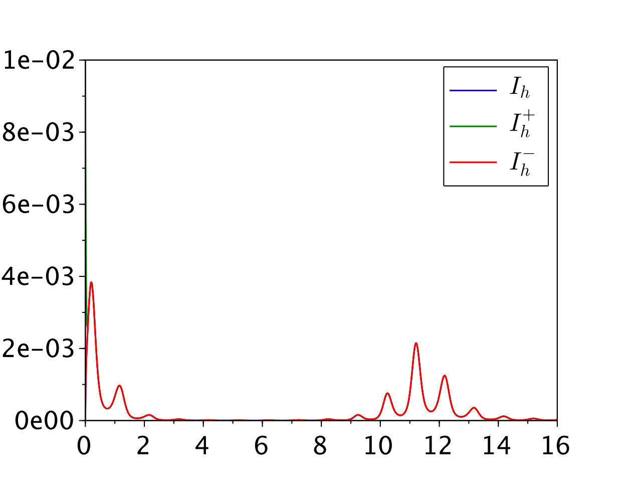 Figure 1
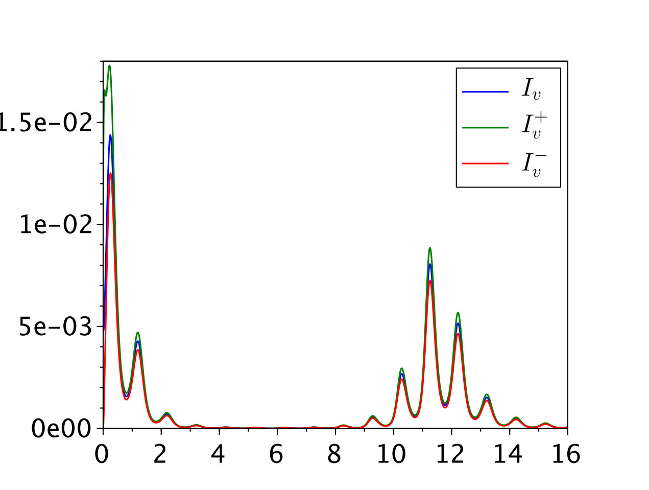 Figure 2
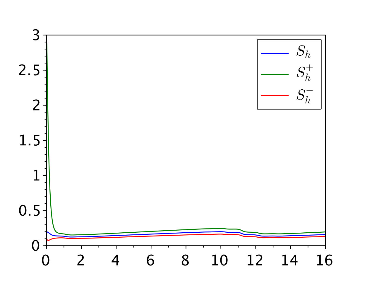 Figure 3
Peer Reviews
No public reviews on file for this paper yet. If you reviewed it on a platform where reviews are public (OpenReview, ICLR, NeurIPS, ICML), you can paste yours below so the community can read it here.
Videos
No videos yet. Explain this paper in a talk, walkthrough, or lecture? Add one.
Taxonomy
TopicsMathematical and Theoretical Epidemiology and Ecology Models · COVID-19 epidemiological studies
Interval observer for uncertain time-varying SIR-SI epidemiological model of vector-borne disease*
Maria Soledad Aronna1 and Pierre-Alexandre Bliman2 *This work was supported by Inria, France and CAPES, Brazil (processo 99999.007551/2015-00), in the framework of the STIC AmSud project MOSTICAW. This investigation was also supported by Fundação Getúlio Vargas in the framework of the Project of Applied Research entitled “Controle da Dengue através da introdução da bactéria Wolbachia”1Maria Soledad Aronna is with Escola de Matemática Aplicada, Fundação Getúlio Vargas, Rio de Janeiro - RJ, Brazil [email protected] 2Pierre-Alexandre Bliman is with Sorbonne Université, Université Paris-Diderot SPC, CNRS, Inria, Laboratoire Jacques-Louis Lions, équipe Mamba, Paris, France and Escola de Matemática Aplicada, Fundação Getúlio Vargas, Rio de Janeiro - RJ, Brazil [email protected]
Abstract
The issue of state estimation is considered for an SIR-SI epidemiological model describing a vector-borne disease such as dengue fever, subject to seasonal variations. Assuming continuous measurement of the incidence rate (that is the number of new infectives in the host population per unit time), a class of interval observers with estimate-dependent gain is constructed, and asymptotic error bounds are provided. The synthesis method is based on the search for a common linear Lyapunov function for monotone systems that represent the evolution of the estimation errors.
I Introduction
Vectors are living organisms that can transmit infectious diseases between humans or from animals to humans. Many of them are bloodsucking insects, which ingest disease-producing microorganisms during a blood meal from an infected host and inject it into a new host during a subsequent blood meal. Vector-borne diseases account for more than 17% of all infectious diseases, causing more than 1 million deaths annually. As an example, more than 2.5 billion people in over 100 countries are at risk of contracting dengue, a vector-borne disease transmitted by some mosquito species of the genus Aedes [18]. Several of the arboviroses transmitted by the latter (Zika fever, chikungunya, dengue) have no satisfying vaccine or curative treatment so far, and prevention of the epidemics is a key to the control policy. In particular, the knowledge of the stock of susceptible individuals constitutes, among others, an important information to evaluate the probability of occurrence of such events.
The dynamics of the dengue transmission is a quite complex subject, due to the role of the cross-reactive antibodies for the four different dengue serotypes [1]. We disregard here this multiserotype aspect, and focus on a basic model of the evolution of a vector-borne disease [4, 7]. The latter is an SIR-SI [11] compartmental model with vital dynamics (see equation (1) below). It describes the evolution of the relative proportions of three classes in the host population: the susceptibles capable of contracting the disease and becoming infective, the infectives capable of transmitting the disease to susceptibles vectors, and the recovered permanently immune after healing; and only the two corresponding classes and in the vector population. The denomination “SIR-SI” of the model recalls this transmission mechanism. The host incidence rate is assumed to be measured.
We are interested in this paper in estimating the repartition of the host and vector populations in time-varying, uncertain, conditions. Our contribution is a class of interval observers [9] providing lower and upper estimates for the state components. Recent progress has been made in the design of interval observers for nonlinear systems, see [15, 6] and a recent survey in [5]. The most recent methods usually involve linearization of the system through the use of the Observer Canonical Form, and then synthesis of interval observer for the corresponding Linear Parameter-Varying system. However the state of the model considered here has dimension 5 and the scalar output is nonlinear with respect to the latter: in practice the complexity of the computations renders this approach intractable here.
An interval observer is therefore designed directly (in the spirit e.g. of [14] and related contributions). We characterize its behavior via the search for common linear Lyapunov functions [12] and by use of the theory of monotone systems [10, 16]. An important feature is that the observer gains are chosen in order to maximize the convergence speed of the Lyapunov functions towards zero. This permits to exploit the epidemic bursts to speed up the state estimation, through estimate-dependent gain scheduling. Error estimates are provided that show, in particular, fast convergence towards the true values in absence of uncertainties on the transmission rates. Notice that related ideas have been applied to an SIR infection model [3]. Similarly to the situation presented in this reference, the epidemiological system studied here is unobservable in absence of infected hosts.
The paper is organized as follows. The model is introduced and commented in Section II. The main assumptions are presented in Section III, where some qualitative results are also provided. The considered class of observers is given in Section IV, together with some a priori estimates, and is proved to constitute a class of interval observers. The main result (Theorem 2) is provided in Section V, where the asymptotic error corresponding to adequate gain choice is quantified. A numerical illustration is presented in Section VI. Some concluding remarks are given in Section VII. Several proofs have been gathered in the Appendix.
II Statement of the problem
Using index for the host population and for the vectors, the SIR-SI model writes
[TABLE]
The parameters , and represent, respectively, the death rates for hosts and vectors, and the host recovery rate. They are assumed to be constant and, as is e.g. the case for dengue, the disease is supposed to induce no significant supplementary mortality in the infected individuals of both populations. The latter are assumed to be stationary, hence , also represent birth rates. Notice that there is no recovery for the vectors, whose life duration is short compared to the disease dynamics.
The parameters and visible in the source terms for the evolution of the infected are, respectively, the transmission rates between infective vectors and susceptible hosts, and between infective hosts and susceptible vectors. The conditions of transmission of the infection display significant seasonal variability (that may relate to changes in the climatic conditions, in the host population behavior…) and we therefore consider time-varying, uncertain, transmission rates. The only measurement of the state components typically accessible to Public Health Services is the host incidence, i.e. the number of new infected hosts per unit time given by . This nonlinear expression of the state variable is the measured output of the model.
By construction, one has , as the proportions verify . This allows to remove one compartment of each population from the model, obtaining the following simplified system:
[TABLE]
When the transmission rates are constant, the evolution of the solutions of system (2) depends closely upon the basic reproduction ratio . The disease-free equilibrium, defined by , (and therefore , ), always exists. When , it is the only equilibrium and it is globally asymptotically stable. It becomes unstable when , and an asymptotically stable endemic equilibrium then appears [7]. In practice, when the parameters are time-varying, complicated dynamics may occur. This is especially the case due to seasonal changes of the climatic conditions, alternating between periods favorable and unfavorable to the occurrence of epidemic bursts.
Our aim in this paper is to estimate at each moment the amount of the three involved populations , based on the measured incidence . An observer for this system has been proposed in the case of constant, known, parameters [17] (assuming the availability of measures of and ), and this is up to our knowledge the unique contribution on the subject. The challenging nature of the problem comes from the fact that when , then and system (2) is therefore unobservable.
III Model assumptions and properties
The host mortality rate (corresponding typically to several tens of years for humans) is assumed very small compared to both the recovery and the vector mortality rates (corresponding typically to some weeks). Our first hypothesis is therefore:
[TABLE]
As said previously, the transmission rates and are supposed to be subject to seasonal variations. We assume moreover that their exact value is not known, but that they are bounded by lower and upper estimates and , available in real-time: for any ,
[TABLE]
Our first result shows that the solutions of system (2) respect the expected bounds.
Lemma 1** (Properties of model (2))**
The solutions of system (2) are such that: if for , then the same properties hold for any . Similarly for strict inequalities.
See in Appendix A a proof of Lemma 1.
IV Observers: definition and monotonicity properties
We now introduce the two following systems, and show in the sequel that, under appropriate conditions, they constitute interval observers for system (2):
[TABLE]
[TABLE]
As can be seen, output injection (the output is ) is used in this synthesis. The time-varying gains in (5a), (5c), (6a), (6c) are yet to be defined.
Lemma 2** (Nonnegativity of the estimates)**
Suppose that for some , the gains are chosen in such a way that, for any :
[TABLE]
Then the solutions of system (5) are such that: if for , then the same remains true for any . Analogously, the solutions of system (6) are such that: if for , then the same remains true for any .
Proof:
Observe that, whenever is close to zero, one has , due to (7). One also has that is nonnegative whenever is in a neighborhood of The same holds for , and this concludes the proof of Lemma 2 for system (5). The proof for (6) is analogous. ∎
Condition (7) imposes special care in the choice of the gains when the estimates come close to zero.
The next result shows that, under sufficient conditions on the gain, equations (5) and (6) provide an interval observer for (2), this is, they provide upper and lower estimates of the three state components.
Theorem 1** (Ordering property of the estimates)**
Assume that the gains are chosen in such a way that, for any , and that condition (7) is verified. Suppose that the solutions of (5), (6) are such that
[TABLE]
for . Then the same holds for any .
To demonstrate Theorem 1, an instrumental decomposition result is now given, whose proof can be found in Appendix B. Lemma 3 indicates in particular that the errors obey some linear positive systems: based on this remark, the proof of Theorem 1 is straightforward.
Lemma 3** (Dynamics of the observer errors)**
The observer errors attached to (5), (6), defined by
[TABLE]
*fulfill, for any , the equations *
[TABLE]
where and are defined in (11).
Moreover, for any , the matrices are Metzler111A square matrix is called a Metzler matrix [8] or an essentially nonnegative matrix [2] if all its off-diagonal components are nonnegative., and the vectors are nonnegative, and null in the absence of uncertainties (that is when and ).
Observe that the matrices and the vectors defined in Lemma 3 depend upon time through the values of the transmission rates and their upper and lower estimates, but also through components of the initial system (2) and of the observers (5) and (6). For brevity this time-dependence is not explicitly shown in (11).
As a last remark, notice that easy computations (not reproduced here) establish that the verification of the Metzler property in Lemma 3 implies that no gain should be introduced in (5b), (6b).
V Observers: convergence properties
We now consider the issue of ensuring fast convergence of the estimates towards zero in the absence of uncertainties. As may be noticed, the dynamics of the (nonnegative) errors (see the 2nd lines of (10a), (10b)) is not modified by the gain choice: the estimates of the proportion of infective hosts converge at a constant rate , which essentially depends upon the recovery rate , as .
Observe that removing the gains and yields converging estimates (see the matrices in (11a), (11b)), with a convergence rate at most equal to the host birth/death rate . But since is very small, it is unsatisfactory for practical matters to settle for such a slow speed of convergence. We provide in Theorem 2 a way to cope with this issue. See Appendix C for a complete proof.
Theorem 2** (Convergence property of the estimates)**
Assume that the initial conditions verify (8) given in Theorem 1. Assume that, for fixed positive scalar numbers the gains fulfill the assumptions of Theorem 1 as well as the conditions:
[TABLE]
where222If in (13a)/(13b), then the selects the other term.
[TABLE]
Then, along any trajectories of (5), (6) one has, for all ,
[TABLE]
where
[TABLE]
are positive definite functions,
[TABLE]
[TABLE]
and
[TABLE]
**
It is easy to verify that it is always possible to find gain values that fulfill (pointwise) (12)-(13). When all assumptions of Theorem 2 are satisfied, inequalities (14) provide guaranteed bounds on the error estimates. In the absence of uncertainties, , , and the functions in (18) are identically null (see Lemma 3): only the first terms remain in the right-hand sides of (14), and the errors converge towards zero exponentially.
The speed of convergence is dictated by the values of the positive (due to Lemma 2) instantaneous convergence rates given in formulas (17). An important point is that convergence may occur with quite a slow pace: when the estimates on the infectives are small, it occurs at the natural rate of system (2). On the contrary, its speed increases with the value of : the observers take advantage of the epidemic bursts to provide tighter estimates more rapidly. By construction , so are at most equal to : the interest of the gain choice made in (12)-(13) is to strive for this performance.
Remark 1** (On noise and unmodeled dynamics)**
Noise in measurement and unmodeled dynamics appearing additively in the right-hand sides of system (2) can be handled without major difficulty (this is omitted here for sake of space). When the latter are upper and lower bounded by some known signals, introducing ad hoc linear expressions of the latter in the right-hand sides of (5), (6) and exploiting the linearity of the Lyapunov functions allows to obtain formulas analogous to (14), with some additional terms in the expression of the functions , .
VI Numerical simulations
The model parameters used for this test are listed in Table I. In order to represent seasonal variations, the transmission rates were taken periodic, , , and the uncertainties were defined by , . The gains were chosen, in accordance with Theorem 2, as
[TABLE]
with , , . Last, the initial conditions were fixed at , , .
Figure 1 represents respectively the corresponding evolution of (in blue) and their lower (in red) and upper (in green) estimates with respect to time (expressed in years). Fast convergence of and towards and respectively is apparent, with quite small residual errors. On the contrary, after a quick decrease, errors on the estimates of stay at relative value of about 20%, due to the uncertainty on the transmission rates.
VII Conclusion
A class of interval observers has been provided for an SIR-SI model of vector-borne disease with time-varying uncertain transmission rates, assuming continuous measurement of the host incidence. The system is unobservable in absence of infectives, and the proposed gain scheduling law speeds up the state estimation during the epidemic bursts. Explicit bounds on the estimation errors have been given, which vanish asymptotically in absence of uncertainties. Numerical test has been provided, demonstrating the expected behavior. The analysis may be extended directly in presence of noise in measurement and unmodeled dynamics.
-A Proof of Lemma 1
Assume that Observe that whenever one has Hence, Let us rewrite (2b)-(2c) in the more convenient form
[TABLE]
Since is always nonnegative, system (20) above turns out to be monotone [10, 16] and, consequently, whenever starting from nonnegative initial values.
On the other hand, if then . Also, whenever , one has Hence, and remain under 1 if their initial values are located under 1.
In order to prove the same properties for the strict inequalities, first integrate (2) to obtain, for any : ; and . From this we can easily deduce that all three variables remain strictly positive if starting from strictly positive initial values, using the previously proved nonnegativity of the three components.
Finally, note that, for any : and . Thus implies the same property for all . The same holds for This ends the proof of Lemma 1.
-B Proof of Lemma 3
Let us first establish (10a). From (2), (5) and the fact that , we get:
[TABLE]
By adding and substracting on the right-hand side of the previous formula, we get
[TABLE]
We now treat the terms in (21) and in (23). Since ,
[TABLE]
Insering (24a) in (21) and (24b) in (23), we get
[TABLE]
which finally yields (10a), together with (11a). The proof is the same for system (10b).
Last, the fact that the matrices are Metzler, and that the vectors are nonnegative and null in the absence of uncertainties, comes directly from the formulas previously proved and the estimates in Lemma 1 and 2. This achieves the proof of Lemma 3.
-C Proof of Theorem 2
We demonstrate here the claimed property for , the case of , being analogous, will not be treated. Throughout this proof we remove the index (5) from the variables and parameters, in order to simplify the notation.
Defining the vector , the (state) function defined in (15a) writes (recall that the error vector has been given in (9a)). Therefore, writing as usual the derivative of along the trajectories, one has, due to formula (10a) in Lemma 3,
[TABLE]
where denotes de identity matrix. Now notice that, with defined in (18a), one has . We show next that
[TABLE]
Given these two facts, one may deduce from (25) that
[TABLE]
which gives (14a) by Gronwall’s lemma and thus achieves the proof. It therefore remains to show (26) in order to complete the proof of Theorem 2.
Let us show that (26) holds when the gains are chosen as prescribed in the statement. Equation (26) can be written as the following system of inequalities, valid for any :
[TABLE]
Using (12a) and (13a) in (27), yields the following equivalent set of inequalities:
[TABLE]
Observe that (28a) is trivially verified. Also, note that
[TABLE]
which yields (in view of (16)) inequality (28b).
Last, by the definition of given in (13a), for any ,
[TABLE]
which implies (28c) since
The inequalities in (26) are thus verified for the chosen values of the parameters. This completes the proof of Theorem 2.
Remark 2
Setting in (27) the gains and to zero and choosing small enough, has values at least equal to (due to the fact that ). Therefore it is always possible to ensure that the convergence speed verifies . On the other hand, since the last term in the right-hand side of (27b) is nonpositive, the value of in (17a) necessarily satisfies for any .
The reference list from the paper itself. Each links out to its DOI / PubMed record.
- 1[1] M Andraud, N Hens, C Marais, and P Beutels. Dynamic epidemiological models for dengue transmission: A systematic review of structural approaches. Plos One , 11, November 2017.
- 2[2] A Berman and RJ Plemmons. Nonnegative matrices in the mathematical sciences . SIAM, 1994.
- 3[3] PA Bliman and B D’Avila Barros. Interval observers for SIR epidemic models subject to uncertain seasonality. In Filippo Cacace et al., editor, Positive Systems , volume 471 of Lecture Notes in Control and Information Sciences . Springer, 2017.
- 4[4] K Dietz. Transmission and control of arbovirus diseases. Epidemiology , pages 104–121, 1975.
- 5[5] D Efimov and T Raïssi. Design of interval observers for uncertain dynamical systems. Automation and Remote Control , 77(2):191–225, 2016.
- 6[6] D Efimov, T Raïssi, S Chebotarev, and A Zolghadri. Interval state observer for nonlinear time varying systems. Automatica , 49(1):200–205, 2013.
- 7[7] L Esteva and C Vargas. Analysis of a dengue disease transmission model. Mathematical biosciences , 150(2):131–151, 1998.
- 8[8] L Farina and S Rinaldi. Positive linear systems: theory and applications , volume 50. John Wiley & Sons, 2011.