Michell trusses in two dimensions as a Gamma-limit of optimal design problems in linear elasticity
Heiner Olbermann

TL;DR
This paper proves that as the weight constraint in a 2D linear elasticity optimal design problem vanishes, the solutions converge to a Michell truss structure, confirming a longstanding conjecture.
Contribution
It establishes the Gamma-limit of the optimal design problem as a Michell truss, providing a rigorous mathematical link between elasticity optimization and truss structures.
Findings
Gamma-convergence of the optimal design problem to Michell trusses
Confirmation of Kohn and Allaire's conjecture
Mathematical characterization of the limit structure
Abstract
We reconsider the minimization of the compliance of a two dimensional elastic body with traction boundary conditions for a given weight. It is well known how to rewrite this optimal design problem as a nonlinear variational problem. We take the limit of vanishing weight by sending a suitable Lagrange multiplier to infinity in the variational formulation. We show that the limit, in the sense of -convergence, is a certain Michell truss problem. This proves a conjecture by Kohn and Allaire.
Click any figure to enlarge with its caption.
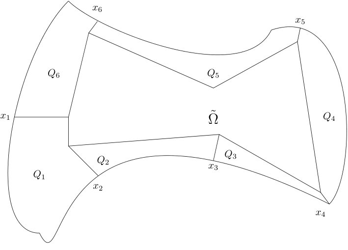 Figure 1
 Figure 2
Peer Reviews
No public reviews on file for this paper yet. If you reviewed it on a platform where reviews are public (OpenReview, ICLR, NeurIPS, ICML), you can paste yours below so the community can read it here.
Videos
No videos yet. Explain this paper in a talk, walkthrough, or lecture? Add one.
Taxonomy
TopicsAdvanced Mathematical Modeling in Engineering · Topology Optimization in Engineering · Composite Material Mechanics
Michell trusses in two dimensions as a -limit of optimal design
problems in linear elasticity
Heiner Olbermann
Universität Leipzig, Germany
Abstract.
We reconsider the minimization of the compliance of a two dimensional elastic body with traction boundary conditions for a given weight. It is well known how to rewrite this optimal design problem as a nonlinear variational problem. We take the limit of vanishing weight by sending a suitable Lagrange multiplier to infinity in the variational formulation. We show that the limit, in the sense of -convergence, is a certain Michell truss problem. This proves a conjecture by Kohn and Allaire.
1. Introduction
The aim of the present article is to derive a certain form of the Michell truss problem from an optimal design problem in linear elasticity in two dimensions. The optimal design problem we consider is the following classical question: Consider an elastic body of given weight loaded in plane stress. Which shape of the body minimizes the compliance (work done by the load)? There exist several different approaches to this problem; here we are going to be concerned with the “homogenization method” that has been developed by Lurie et al. [22], Gibiansky and Cherkaev [17], Murat and Tartar [26], Kohn and Strang [20], and others. The homogenization method rephrases the compliance optimization problem as a two-phase design problem, and then enlarges the set of permissible designs via relaxation. We refer the interested reader to Allaire’s book [1] for a more thorough account of the method.
On a formal level, it has been noted by Allaire and Kohn [2] that the relaxed formulation of the problem leads to a different variational problem in the limit of vanishing weight, namely a certain variant of the Michell truss problem (see also [28, 4]). This problem was first stated by Michell in 1904 [24]. Michell trusses are elastic structures that consist of linear truss elements, each of which can withstand a certain tensile or compressive stress. The variational problem consists in finding the Michell truss of least weight that is admissible in the sense that it resists a given load. Michell himself already knew that this problem has no solution in general, and relaxation is required to assure existence of solutions. Since this day, the theory of Michell trusses has been very popular in the engineering and mathematics community. We refrain from attempting to give a comprehensive list of the relevant literature, and refer the reader to [19, 27].
In the present article, we are going to cast the formal observations by Kohn and Allaire into a rigorous statement. More precisely, we are going to prove that the Michell truss problem is the limit of the compliance minimization problem in linear elasticity for vanishing weight in the sense of -convergence [9].
The plan of the paper is as follows: Section 2 below is supposed to give the reader a quick overview over the setting and main result. It consists of four Subsections: In Sections 2.1 and 2.2, we are going to state the compliance minimization problem for positive weight and the Michell problem respectively. In Section 2.3, our aim is to give the reader a good idea of our main result as quickly as possible, without too many preparatory definitions. This is why we first state a special case of our main theorem, Theorem 2.2. In Section 2.4, we give a short explanation of the form of the variational formulation of the compliance minimization problem that we had presented in Section 2.1. In Section 3, we are going to collect some results from the literature. In Section 4, we explain the manner in which we use Airy potentials for the solution of elasticity problems, and we state our main -convergence result, Theorem 4.7. Section 5 contains the proof of the compactness and upper bound part of Theorem 4.7, and Section 6 contains the proof of the lower bound. The appendix consists of two parts: In Section A, we prove some facts on the relaxation of integral functionals whose integrands depend on second gradients, which we were unable to find in the literature. In Section B, we derive the 2-quasiconvexification of the integrand in the compliance minimization problem.
Notation
The symbol “” is used as follows: A statement such as “” is shorthand for “there exists a constant such that ”. The value of may change within the same line. For , we also write .
2. Setting and (a special case of the) main result
In the present section, our aim is to present first, the optimal design problems in linear elasticity, second, the Michell truss problem in its variational form, and third, a special case of our main theorem that links these problems via -convergence. On the one hand, this special case does not require a lot of preparatory definitions, and on the other hand, it is not much weaker than the full result.
For a bounded open set , and , the Sobolev space is defined by its norm
[TABLE]
where the sum runs over multiindices with and . For , we use the notation
[TABLE]
For the spaces with homogeneous boundary conditions, we use the notation
[TABLE]
The fractional Sobolev spaces with , and are defined by the Gagliardo norm,
[TABLE]
For compact, -rectifiable subsets , we define the norms , by a suitable cover of by the ranges of Bilipschitz maps, and we write . The dual of is denoted by , and the dual of is denoted by .
We write . On , we introduce a scalar product by
[TABLE]
We will also use the notation for .
In the present paper, we are going to derive a result for bounded open sets . More precisely, the symbol will be reserved for sets satisfying the following definition:
Definition 2.1**.**
From now on, we assume that has the following properties:
- (i)
* is open, bounded, connected and simply connected*
- (ii)
There exists a finite number of points , , with pairwise disjoint neighborhoods of and -diffeomorphisms such that , and .
- (iii)
* is away from .*
The purpose of (ii) and (iii) above is that the operator , is surjective, where denotes the outer unit normal to , see Theorem 3.10 below. We will denote the outer unit normal of by , and define a tangent vector . We denote the tangential derivative by , and the normal derivative by .
2.1. The compliance minimization problem
For , let be defined by
[TABLE]
In the following, the parameter is a Lagrange multiplier for the weight of the two-dimensional elastic structure. Taking the limit of vanishing weight corresponds to the limit . We define the functionals for finite with boundary conditions fixed by the choice of some . The space of allowed stresses is given by
[TABLE]
where denotes the unit outer normal of . The integral functional for finite is given by
[TABLE]
For explanation of the fact that the traditional form of compliance minimization is equivalent to the minimization of , see Section 2.4.
2.2. The Michell truss problem
For the definition of the limit functional, we need to collect some more notation.
For any Borel set , let denote the set of signed Radon measures on . We denote by the valued Radon measures on . Furthermore, let denote the space . For , let denote the total variation measure (see Section 3.1). For , we have by the Radon-Nikodym differentiation Theorem (see Theorem 3.1 below) that for -almost every , the derivative exists. For any one-homogeneous function and any , we may hence define
[TABLE]
This is a well defined Borel measure.
Now let be open. Let denote the dual of , i.e., the space of valued distributions whose support is compactly contained in . Let , . We say that if and only if
[TABLE]
for every . Here and are viewed, respectively, as a measure and a distribution on supported on . If has support in the boundary , then this induces a boundary condition for . Just as in the equation above, the notation will denote the pairing of topological vector spaces with their dual in the sequel. It will always be clear from the context which pairing is meant. For and , we say that if the equation holds for every row, for .
For , let denote the eigenvalues of . We set
[TABLE]
We will repeatedly use the following estimates:
[TABLE]
Note that is sublinear and positively one-homogeneous.
For , , we write and . Again, for and , we say that if the equation holds for every row.
Now let be as in Definition 2.1. For , let the space of permissible stresses be given by
[TABLE]
With these preparations, we are ready to define the Michell problem for for traction boundary values ,
[TABLE]
For a motivation of this functional in the context of structural optimization, we refer to [1, 2].
2.3. Gamma convergence
We want to approximate the functional by the functionals in the sense of -convergence. We assume that satisfies Definition 2.1. We introduce the trace operators
[TABLE]
For the properties of the trace operators, see Section 3.4 below.
As a special case of our main theorem, we have that for ,
[TABLE]
More precisely:
Theorem 2.2**.**
Let satisfy Definition 2.1 and let .
- (i)
Compactness:* Let be such that . Then there exists a subsequence (no relabeling) and such that weakly * in the sense of measures.*
- (ii)
Lower bound:* If weakly * in the sense of measures, then*
[TABLE]
- (iii)
Upper bound:* For every there exists a sequence such that weakly * in the sense of measures and .*
Remark 2.3**.**
- (i)
For the sake of simplicity, we have here set the same boundary conditions for the approximating and the limit problem. Actually, one would like to obtain a larger class of allowed “boundary conditions” for the limit problem. For example, one would like to consider , where , for and denotes the distribution defined by . These boundary values are the ones that one considers in the Michell problem, see **[5]**. Distributions of this type are not in , but they do belong to , which at first glance might look like the “natural” space for the boundary conditions of the limit problem. In our main theorem, we will allow boundary values from a certain subset of in the limit problem. In particular, this subset contains the aforementioned “delta-type” distributions, provided that the applied forces do not act tangentially, see Lemma 4.4. The functions in this space will be approximated by boundary values .
- (ii)
The main idea of our proof can be summarized as follows: By the well-known representation of divergence free stresses via Airy potentials, we can formulate the variational problems for finite and vanishing weight as the minimization of integral functionals in the spaces and respectively, where the latter denotes the space of functions of bounded Hessian, i.e., the space of functions such that the distributional derivative defines a vector-valued Radon measure. We may then use the blow-up technique developed by Fonseca and Müller **[15, 14, 3]** and the results by Kohn and Strang **[20]** and Allaire and Kohn **[2]** to prove the lower bound part of the -convergence result. For the construction of the upper bound, we use approximation and relaxation results that are well known to specialists. Nevertheless, for some of them, we could not find a proof in the literature and provide them here.
- (iii)
In their formal derivations of the Michell truss problem in **[2]**, Allaire and Kohn also discussed the three-dimensional case. We are not able to say anything new about this case: The representation of divergence free stresses via Airy potentials is limited to two dimensions.
- (iv)
We restrict ourselves to the case of vanishing Poisson ratio for the sake of simplicity and readability. The interested reader will be able to generalize our results without difficulty to a general “soft” isotropic phase, defined by the elasticity tensor with
[TABLE]
where are the shear and bulk modulus respectively, and denotes the set of linear operators . In that case, the functionals for finite are given by
[TABLE]
where
[TABLE]
and the limit functional is given by . It suffices to take the formulas for the quasiconvex envelope for from **[2]**, and adapt our proof accordingly.
2.4. Derivation of the variational form of the compliance minimization problem
We give a brief derivation of the compliance minimization problem in its variational form,
[TABLE]
starting from the standard formulation in linear elasticity. What we present here is a subset of the derivation by Allaire and Kohn, see [1] for more details.
As before, let . Consider an elastic body , characterized by its elasticity tensor , where we assume that is invertible. We remove a subset from the elastic body and the new boundaries from that process shall be traction-free. The resulting linear elasticity problem is to find such that
[TABLE]
where . The compliance (work done by the load) is given by
[TABLE]
where is the unique solution to the linear elasticity system above. We want to minimize the compliance under a constraint on the “weight” . We do so by the introduction of a Lagrange multiplier , and are interested in the minimization problem
[TABLE]
Taking the limit of vanishing weight corresponds to the limit . We rephrase the problem by considering space-dependent elasticity tensors of the form , where . The elasticity system from above becomes
[TABLE]
Now the compliance is a functional on the set of permissible elasticity tensors, and is given by
[TABLE]
where is the solution of (5). By the principle of minimum complementary energy, we have that the compliance can be written as
[TABLE]
where
[TABLE]
and is a solution of the PDE
[TABLE]
i.e., . We see that the compliance minimization problem can be understood as the variational problem of finding the infimum
[TABLE]
Of course, the compliance of a pair is infinite if there exists a set of positive measure such that and on . Hence the above variational problem is equivalent with
[TABLE]
where has been defined in (4). As is well known, the variational problem (6) does not possess a solution in general and requires relaxation. For simplicity, we assume here that is the identity on , see Remark 2.3. Then (6) is just the variational problem .
3. Preliminaries
For the proof of our main result, we are going to rely heavily on two sets of results from the literature: On the one hand, on the results on optimal design in the “relaxed formulation” [20, 2, 1], and on the other hand, on the blow-up technique for the derivation of relaxed functionals and -limits developed by Fonseca and Müller [13, 3, 14]. In order to present them, we need to review some basic facts about measures, functions and quasiconvexity.
In the following, let be open and bounded.
3.1. Measures
At the basis of the blow-up argument that we use in the present work is a refinement of the well known Radon-Nikodym differentiation theorem:
Theorem 3.1** (Proposition 2.2 in [3]).**
Let be Radon measures in with . Then there exists a Borel set with such that for any we have
[TABLE]
for any bounded convex set containing the origin. Here, the set is independent of .
Let for . We say that weakly * in the sense of measures if
[TABLE]
It is a well known fact that if , then there exists a weakly * convergent subsequence.
The next result concerns the convergence of positively one-homogeneous functions of measures. The statement below is contained in Theorem 1.15 in [12].
Theorem 3.2**.**
*Let be positively one-homogeneous and continuous, and let , , such that , weakly
- in the sense of measures. Then*
[TABLE]
3.2. and functions
The space of functions of bounded variation is defined as the set of functions that satisfy
[TABLE]
In this case, the map defines a vector valued Radon measure, which is denoted by .
According to the Theorem 3.1, we have the following decomposition of the measure for ,
[TABLE]
where and is the so-called singular part of .
The following theorem determines the structure of blow-ups of functions:
Theorem 3.3** (Theorem 2.3 in [3]).**
Let and for a bounded convex open set containing the origin, and let be the density of with respect to , . For , assume that with , , , and for let
[TABLE]
Then for every there exists a sequence converging to 0 such that converges in to a function which satisfies and can be represented as
[TABLE]
*for a suitable non-decreasing function , where and . *
We will also need Alberti’s rank-one theorem:
Theorem 3.4**.**
Let . Then is rank-one.
For later reference, we also mention that for , we have as a consequence of the classical Sobolev embeddings, that for almost every , we have
[TABLE]
Here, we have used the notation .
The space of functions of bounded Hessian is defined as
[TABLE]
It can be made into a normed space by setting
[TABLE]
We say that a sequence converges weakly * to if in and weakly * in .
The space has been investigated first in [10, 11]. In particular, these papers contain theorems about compactness and extension properties of this space. The first theorem that we cite is a weakened form of Theorem 1.3 in [11]:
Theorem 3.5**.**
Let be a bounded sequence in . Then there exists a subsequence (no relabeling) and such that
[TABLE]
In two dimensions, functions in are continuous:
Theorem 3.6** ([10], Theorem 3.3).**
Let with boundary. Then
[TABLE]
3.3. Relaxation of integral functionals that depend on higher
derivatives
In the proof of the upper bound of Proposition 15, we will need a relaxation result for integral functionals that depend on second gradients. This is the case in Theorem 3.7 below.
A function is called -quasiconvex if
[TABLE]
see [23]. The so-called -quasiconvexification of is given by the right hand side above,
[TABLE]
As is well known, in the case , one obtains the relaxation of integral functionals by replacing by its 1-quasiconvexification . Concerning higher , there exist some relaxation results in the literature, but we could not find any theorems that fit our situation. In particular, Theorem 1.3 in [6] deals with the case of the relaxation of Caratheodory functions. In our case, where the integrand only depends on the second gradient, this means that continuity of the integrand with respect to is required. We are interested in the non-continuous case , so we cannot use this theorem. The following theorem suits our purpose, and we prove it in the appendix:
Theorem 3.7**.**
Let , and let such that
[TABLE]
Let satisfy Definition 2.1, and let . Let and . Then there exists with
[TABLE]
Remark 3.8**.**
The theorem can be straightforwardly generalized to the case of higher derivatives, if in Definition 2.1 one replaces -regularity with -regularity of in the appropriate sense. Another straightforward generalization is the case of general dimension of the domain . Moreover, (simple) connectedness and boundedness of are not necessary here.
We will need to determine the 2-quasiconvexification of . In principle this is contained in [20, 2]. However we could not find a clear statement in the literature, so we give a proof of the following theorem in the appendix.
Theorem 3.9**.**
We have
[TABLE]
3.4. Trace and extension operators
Recall that we assume that satisfies Definition 2.1. The trace operator
[TABLE]
is linear surjective as a map (see [16]) and also as a map (see [25]). For the spaces and , it also makes sense to consider the operator
[TABLE]
The following theorem combines statements from Chapter 1.8 of [21] and Chapter 2 as well as the appendix of [10].
Theorem 3.10**.**
- (i)
The operator is linear surjective both as a map
[TABLE]
and as a map
[TABLE]
- (ii)
There exist continuous right inverses , defined as maps
[TABLE]
and
[TABLE]
Remark 3.11**.**
- (i)
The norm on is the one induced by ,
[TABLE]
Note that , see the appendix of **[10]**. This fact together with the theorem explains our choice of assumptions on the boundary conditions in our main theorem; see equations (15) and (17) below.
- (ii)
In **[10]**, the statement on the surjectivity of the trace operator is only made for -regular boundary. For the sake of brevity, we only sketch the changes of that proof that have to be made to show that the claim also holds true for satisfying Definition 2.1. In Proposition 1 of the appendix of **[10]**, it is shown that for , there exists such that , . The proof works by an explicit construction, modifying an idea by Gagliardo. In fact, using the explicit formulas for and its partial derivatives that are given in the proof, one easily deduces that . Hence, one may use the Proposition twice to obtain that vanishes on , and whose normal derivative agrees with a given on . With this slightly more general version of the Proposition, the proof of Theorem 1 in the appendix of **[10]**, which states the surjectivity of the trace operator, can be extended to the case where satisfies Definition 2.1 without additional changes: One uses a suitable cover of the boundary by open sets, an associated partition of unity and -regular diffeomorphisms that reduce the problem to the situation of the proposition.
We have the following Poincaré inequality for :
Lemma 3.12**.**
Let , , , then we have
[TABLE]
Proof.
By the Poincaré inequality for functions (see [30] Chapter 5) we have
[TABLE]
and
[TABLE]
This proves the claim. ∎
Next, we quote a general extension result from [29]. In the following, we slightly change a definition from [29]:
Definition 3.13**.**
Let be open and bounded. We say that the boundary is said to satisfy minimal conditions if
- (i)
There exists a cover of by a finite number of open sets
- (ii)
For every , can be represented as the graph of a Lipschitz function with .
Note that if satisfies Definition 2.1, then also satisfies the minimal conditions.
Theorem 3.14** (Theorem 5 and 5’ in Chapter 6 of [29]).**
Let such that satisfies the minimal conditions. Then there exists an extension operator
[TABLE]
that is continuous as a map for every and every . Moreover, the norm of this operator only depends on and on the maximum of the Lipschitz constants of the functions that appear in Definition 3.13 (ii).
4. Airy potentials and boundary conditions
In the present section, we assume that satisfies Definition 2.1.
4.1. Airy potentials
Here we are going to rephrase the compliance minimization problem and the Michell problem. We use the representation of divergence free stresses in two dimensions by Airy potentials. We recall that for , the cofactor matrix is defined by
[TABLE]
Note that in two dimensions, we have .
In the compliance minimization problem, we say that is an Airy potential for if
[TABLE]
Note that in such a situation, we have . Since is linear on two by two matrices, the object is well defined for . We say that the function is an Airy potential for if is a neighborhood of , and
[TABLE]
as elements of . Our definitions of Airy potentials make sense by the Poincaré Lemma; this statement is made precise in the following lemma.
Lemma 4.1**.**
We have
[TABLE]
and
[TABLE]
Proof.
The inclusion is obvious. For the opposite inclusion, let with . Let be a standard mollifier, i.e., , , , and . On , set . Note that we have with on . For small enough, is simply connected, and by the Poincaré Lemma there exists such that . For every , there exists an open square with center . On , we have
[TABLE]
Using , one easily obtains on , and hence on all of . Again by the Poincaré Lemma there exists such that on . Of course, the sets have Lipschitz boundary. Moreover, there exist open sets such that for small enough, can be represented as the graph of some Lipschitz function , and the Lipschitz constants of are uniformly bounded. By Theorem 3.14, we may extend to such that
[TABLE]
where does not depend on . After subtracting suitable affine functions, we may assume
[TABLE]
From (11) and the Poincaré inequality in (see [10]) it follows
[TABLE]
By Theorem 3.5, we obtain that there exists such that in , with . This proves the first statement. The second statement is proved in the same way, using Theorem 3.14 for the extension , and weak compactness of the resulting bounded sequence in . ∎
4.2. Boundary values
We say that is balanced if
[TABLE]
It only makes sense to consider balanced traction boundary values, as can be seen from the following well known lemma (see e.g. [5]):
Lemma 4.2**.**
If , then is balanced.
Proof.
Assume . Taking or and testing these functions against the identity (see (1)), we obtain
[TABLE]
Secondly, taking as a test function, we get
[TABLE]
The latter holds since has values in the symmetric matrices. This proves the lemma, since for every , there exists such that . ∎
For certain , we now define two integrals . Let be fixed, , and let denote the positively oriented simple Lipschitz curve that satisfies
[TABLE]
Obviously, is a Bilipschitz homeomorphism.
For with , we may define its first integral by
[TABLE]
where is chosen such that . We may extend this definition to with , where is the function defined by for all : We let (to be thought of as the first integral of ) be defined by
[TABLE]
For vector valued arguments, we may define by its action on the components of its argument.
We recall that denotes the unit outer normal of , and . Let these objects be understood as functions in . If with for , then can be understood as an element of , by
[TABLE]
If we assume furthermore , we can define the first and second integrals and by
[TABLE]
In order to make the transition between stresses and their Airy potentials, the following definition will be convenient: Let
[TABLE]
We make into a topological vector space by letting the topology on be the strongest one that makes the following map continuous:
[TABLE]
Remark 4.3**.**
- (i)
The requirements for the existence of , namely that
[TABLE]
precisely express that has to be balanced, for all , . To see that for all is equivalent with the second equation in (13), we observe that
[TABLE]
- (ii)
The space is a replacement for ; the latter is slightly too large for our purposes. In the formulation of the compliance minimization problem via Airy potentials, we need to translate the integrals of the boundary values into boundary values of a function in and its normal derivative. This is not possible for , firstly because , and secondly because . Nevertheless, with our choice of we have and furthermore contains balanced finite sums of delta distributions that do not contain applied forces tangential to . For the precise statement, see Lemma 4.4 below.
The upcoming lemma only serves to prove the claim made in the previous remark and can be skipped by the reader who is only interested in the statement and proof of the main theorem.
For and , we write if there exists such that either or . This is the case, for example, if is the tangent vector to in a point where the curvature does not change sign. (If the curvature changes sign at , then .) If is not near , then the set is larger, see Figure 1.
Lemma 4.4**.**
For let and such that , and additionally
[TABLE]
Then is balanced, and .
Proof.
Using the definitions, the fact that is balanced is obvious. With the notation we have introduced above, and the assumption for , we have
[TABLE]
Hence is a piecewise constant function . Let denote the value of on the arc connecting and in (counterclockwise). Furthermore we note that with . For every , choose at least so small that
[TABLE]
For , there is exactly one out of the two points that is contained in . Denote this point by . Let be a simply connected polygonal domain with for . Let denote the open subset of that is bounded by , , and , see Figure 2.
On , we may define almost everywhere by setting
[TABLE]
This makes affine on each subset , and we claim that there exists a continuous extension to . Indeed, we need to check continuity only at the boundaries . For , we have
[TABLE]
This proves the existence of the continuous extension of to . Let be a triangulation of , and extend to a function that is affine on each triangle of and continuous on . Since piecewise affine continuous functions are of bounded Hessian, we have , and
[TABLE]
Hence , and the lemma is proved. ∎
For , we have that implies on . If additionally for some , then . This implies that the integral is equal to up to a constant, and is equal to up to an affine function. The following lemma restates these observations for the non-smooth case.
Lemma 4.5**.**
Let , , and let be a neighborhood of , such that , and . Then there exists and an affine function such that
[TABLE]
The same conclusion holds true if , , and with .
Proof.
To prove the first claim, we show that there exists and some vector such that
[TABLE]
where the right hand side is understood in the sense of traces of functions. To prove this claim, let . Then we have
[TABLE]
Let denote the restriction of the jump part of to . Then we have
[TABLE]
Using Theorem 3.4 and the symmetry of , we have that is -almost everywhere parallel to , and we may write . Hence,
[TABLE]
By the Gauss’ Theorem for functions (see e.g. [18]), we have that
[TABLE]
Hence, we have
[TABLE]
This proves (14) and hence the first claim. Next we observe that
[TABLE]
which proves the second claim. Finally, the situation is just a special case of what we have just proved, by extending to some , where is some neighborhood of , and , which is possible by Theorem 3.14. ∎
4.3. Statement of the main theorem
First we will state a proposition that is basically equivalent to our main theorem, using Airy potentials and the most general boundary values that are allowed within this framework.
For let the functional be defined by
[TABLE]
Furthermore, for , let the functional be defined by
[TABLE]
In the statement of the following theorem, we use the standard norm on the Cartesian product , i.e.
[TABLE]
Proposition 4.6**.**
Let satisfy Definition 2.1, and assume that
[TABLE]
- (i)
Compactness:* Let be such that . Then there exists a subsequence (no relabeling) and such that weakly
- in .*
- (ii)
Lower bound:* If weakly * in , then*
[TABLE]
- (iii)
Upper bound:* For every there exists a sequence such that weakly * in and .*
With the proposition at hand, we can prove our main theorem, which contains Theorem 2.2 as a special case.
Theorem 4.7**.**
Let satisfy Definition 2.1, and assume that
[TABLE]
- (i)
Compactness:* Let be such that . Then there exists a subsequence (no relabeling) and such that weakly * in the sense of measures.*
- (ii)
Lower bound:* If weakly * in the sense of measures, then*
[TABLE]
- (iii)
Upper bound:* Assume that contracts nicely. For every there exists a sequence such that weakly * in the sense of measures and .*
Remark 4.8**.**
The reason for the assumption here, and for the analogous assumption in the Proposition, is technical. This allows us to control the behavior of boundary layers in the upper bound construction, and gives a convenient estimate for error terms appearing in the proof of the lower bound, see the proof of Proposition 15. However, these assumptions are not a restriction, in the sense that every with possesses an approximating sequence with these properties.
Proof.
Recall the definition of the “integrals” from (12). We may assume that are balanced, since otherwise or by Lemma 4.2. By Remark 4.3 (i), the requirements for the existence of , are met. Now we set
[TABLE]
With these definitions, (17) implies (15).
For the compactness part, assume that . Using Lemma 4.1, we obtain a sequence in with . By Proposition 15, we obtain weak
- convergence of to .
For the lower bound part, we assume with weakly * in and . We may assume , since otherwise . Using Lemma 4.1, let and such that and . By Lemma 4.5, we may assume that by the addition of suitable affine functions, we have
[TABLE]
This implies and , and hence the lower bound follows from the lower bound part of Proposition 15.
For the upper bound part, let . Applying Lemma 4.1 and Lemma 4.5 we have that after the addition of an affine function, with . The upper bound part of Proposition 15 and (19) immediately yield the desired recovery sequence. ∎
The rest of this paper is concerned with the proof of Proposition 15.
5. Proof of compactness and upper bound
In this section and the next, we use the notation
[TABLE]
By Theorem 3.9, we have
[TABLE]
Proof of compactness in Proposition 15.
We claim that for ,
[TABLE]
By , this implies
[TABLE]
By Lemma 3.12, we obtain that is a bounded sequence in . By Theorem 3.5 we obtain that a subsequence converges weakly * in . It remains to prove (20).
Let . Let denote the absolute values of the eigenvalues of . For we have
[TABLE]
Hence we have
[TABLE]
If , then
[TABLE]
Combining these two cases, we obtain (20) which proves the compactness part of the theorem. ∎
Proof of the upper bound in Proposition 15.
By Theorem 3.10, the application of the right inverse of the trace operator to and yields a sequence in and such that
[TABLE]
By Theorem 3.14, we may extend and to all of such that
[TABLE]
Let be defined by
[TABLE]
Let be some neighborhood of , and let be a -diffeomorphism, such that , where is a convex polygon that contains the origin. Such a map exists by our assumptions on , see Definition 2.1. Choose such that
[TABLE]
for all small enough. For such , we set
[TABLE]
and
[TABLE]
Note that and on . Additionally, we claim that in the limit , we have
[TABLE]
To prove this claim, we observe that and uniformly as . Now we have
[TABLE]
where by , we mean the Radon measure that is defined by
[TABLE]
From the uniform convergences , and , the claim (24) follows.
We let be such that and , and . Next we set
[TABLE]
and by the properties of , we have
[TABLE]
Furthermore, there exists a constant such that
[TABLE]
We set
[TABLE]
and define the recovery sequence by
[TABLE]
Our choice of implies that
[TABLE]
From (23) and Theorem 3.5, we see that converges weakly * in to the function
[TABLE]
Next let
[TABLE]
[TABLE]
Let
[TABLE]
For every , we have that
[TABLE]
where we have used the assumption (15). This implies, using the non-negativity of ,
[TABLE]
where we have used Theorem 3.2 in the last step, and the fact that
[TABLE]
Taking the limit in the estimate (26), we obtain
[TABLE]
On the right hand side above, has to be understood as the trace of . By Theorem 3.6, we have that is continuous. In particular, we must have , and hence
[TABLE]
which implies
[TABLE]
By Theorem 3.7, we may find with on such that it satisfies
[TABLE]
This implies that in . Also, we have
[TABLE]
By the compactness part, it follows that weakly * in . This proves that is the required recovery sequence. ∎
6. Proof of the lower bound
Lemma 6.1**.**
Let be open and bounded, and in with . Then in .
Proof.
By the Poincaré inequality,
[TABLE]
For large enough we may assume , and hence . In particular, we have
[TABLE]
Now by for and , we have
[TABLE]
This proves the lemma. ∎
Lemma 6.2**.**
- (i)
Let be open and bounded, , and in as . Then
[TABLE]
- (ii)
Let with and let be a cube such that one of its sides is parallel to , and let such that
[TABLE]
for some and . Furthermore let , and . Then
[TABLE]
Proof of (i).
We may assume . We claim that for , , we have
[TABLE]
Indeed, by the sublinearity of , we may assume and . Using the fact that , we can make the following case distinction:
- Case 1:
If , then we have
[TABLE]
- Case 2:
If , then . Additionally, by (22), we have . This allows us to estimate
[TABLE]
- Case 3:
If , then again by (22), we have , and hence
[TABLE]
This proves (29). Hence we have
[TABLE]
and there exists a non-negative Radon measure such that
[TABLE]
Let be an increasing sequence of subdomains s.t.
[TABLE]
and let be smooth cutoff functions with , , . We set
[TABLE]
By the quasiconvexity of , we have
[TABLE]
This implies
[TABLE]
We estimate
[TABLE]
where we have used (29) in the first inequality. Subtracting the inequality (30) from , and additionally using (31), we obtain
[TABLE]
We have , and hence by Lemma 6.1, we have
[TABLE]
Sending in (32) and using (33) and the non-negativity of , we obtain
[TABLE]
Summing up from to and dividing by , we get
[TABLE]
Sending , we obtain the desired result. ∎
Proof of (ii).
The proof of Lemma 4.3 (ii) in [3] can be copied word by word; except for the last step, where instead of Lemma 4.3 (i) in that reference we use part (i) of the present lemma. ∎
Proof of the lower bound in Proposition 15.
We may assume and after choosing an appropriate subsequence, we may also assume .
Let be the right inverse of the trace operator from Theorem 3.10, and let be the extension operator from Theorem 3.14. Letting , we have that defined by
[TABLE]
satisfies . Setting and , we have
[TABLE]
By assumption (15) and the continuity of we have
[TABLE]
The latter implies in particular that is equiintegrable, and hence we obtain from (34) and (35) that
[TABLE]
From now on we write . By assumption, the sequence is bounded, and hence
[TABLE]
by (34) (with ). Also, by for all , we have
[TABLE]
By (37) and (38) and the compactness theorems for functions and Radon measures respectively, there exists a subsequence of (no relabeling), a measure and with on , such that
[TABLE]
By Theorem 3.1 there exists an measurable function and a measurable function such that
[TABLE]
We are going to show
[TABLE]
We claim that this implies (16). Indeed, recall that the right hand side in (16) reads
[TABLE]
see equations (27) and (28) in the proof of the upper bound. Let . By (36), the left hand side of (16) is equal to
[TABLE]
Now we see that (39) and (40) imply , and hence prove the lower bound part. It remains to show (39) and (40).
First we prove (39). Let . For -almost every , we may choose a sequence converging to zero, such that for every . When we write in the sequel, we actually mean the limit for such a sequence. For every , we have
[TABLE]
Note that by Theorem 3.1 we have
[TABLE]
For small enough, define by
[TABLE]
Furthermore let . Using a change of variables, the Cauchy-Schwarz inequality and (7), we have
[TABLE]
By (41) and (42), it is possible to choose a sequence and a subsequence (no relabeling) such that with
[TABLE]
Noting , we obtain from Lemma 6.2 that
[TABLE]
This proves (39).
We turn to the proof of (40). By Theorem 3.1 we have that for -almost every , there exist with such that for any open bounded convex set containing the origin, we have
[TABLE]
Let denote the cube of sidelength one, with one axis parallel to :
[TABLE]
Furthermore, let . From now on, let the limit be understood only to involve a sequence such that for all . By the definition of , we have
[TABLE]
We define
[TABLE]
Let . By Theorem 3.3 there exists such that with
[TABLE]
we have and
[TABLE]
By the convergence in , we have , and hence
[TABLE]
By (43) and (44), we can choose a subsequence and a sequence such that
[TABLE]
Now let . Then we have and
[TABLE]
Hence using Lemma 6.2 (ii) it follows
[TABLE]
Sending proves (40) and completes the proof of the lower bound. ∎
Appendix A Proof of Theorem 3.7
In analogy to the proof of the relaxation leading to 1-quasiconvex integrands, we first need to prove an approximation lemma. This is slightly more complicated here than in the case of 1-quasiconvexity, since we cannot use the approximation by finite elements here, which is possible there (see [7]). Instead, we are going to need Whitney’s extension theorem, that we quote here in a version that can be found in Stein’s book [29]. Let . Let the Greek letters denote multiindices. We will write , , and . Furthermore, for , we write . We shall say that a function belongs to if there exists a collection of real-valued functions and a constant such that
[TABLE]
and
[TABLE]
for all and all multiindices with . The set is a normed space, where the norm of is given by the smallest constant such that the above relations hold true.
Theorem A.1** (Theorem 4 in Chapter 6 of [29]).**
Let be a non-negative integer and let be closed. Then there exists a continuous extension operator . The norm of this mapping has a bound that is independent from .
For a closed set , let denote a regularized distance function, that is, a function with the property that there exists a constant such that
[TABLE]
Such a regularized distance function exists by Theorem 2 of Chapter 6 in [29]. We will use it to construct suitable cutoff functions in Lemma A.2 below. This lemma is a preparation for the approximation lemma, Lemma A.3 below.
Let such that for and for .
Lemma A.2**.**
Let , , a sequence in that converges strongly to for , and let
[TABLE]
be a closed set of positive measure, and such that and on . Furthermore let
[TABLE]
Then and on , and
[TABLE]
Proof.
The first claim is obvious. To show the second claim, it suffices to show that , since and its gradient vanish on . This is a straightforward computation, that estimates the integral over in the “bulk” and in boundary layer
[TABLE]
where the constant is chosen appropriately. The contribution of the bulk vanishes in the limit due to the assumption. Writing and its gradient as integrals in -direction in the set for and using Fubini’s theorem, the proof that the contribution of the boundary layer vanishes in the limit is a straightforward but lengthy computation that we omit here for the sake of brevity. The third claim is an immediate consequence of the integrability of and the strong convergence in . ∎
Lemma A.3**.**
Let satisfy Definition 2.1, and let . Furthermore let and . Then there exists and such that is the union of mutually disjoint closed cubes, is piecewise a polynomial of degree on , and furthermore
[TABLE]
Proof.
Let . We may extend to such that
[TABLE]
Also, may be understood as an element of by a trivial extension. Let be an open cover of , let be a subordinate partition of unity, and let , , be a set of diffeomorphisms such that and . (Such exist by the assumption on .)
Let with , and . For every , we have that
[TABLE]
By the previous lemma, there exists such that on ,
[TABLE]
and additionally,
[TABLE]
Setting , we obviously have that on , and
[TABLE]
Setting
[TABLE]
we have on and
[TABLE]
and hence we may fix such that
[TABLE]
Note that is closed and .
Let to be chosen later, and let , be mutually disjoint closed cubes of sidelength contained in such that
[TABLE]
This is always possible assuming that is small enough. Let denote the midpoint of . Then we define to be the Taylor polynomial of degree two at on each ,
[TABLE]
Let . We claim that there exists an extension of from to such that . In order to prove our claim, we invoke Theorem A.1 with . We verify that : Firstly, we have for all and all multiindices with ,
[TABLE]
where the constant depends on . Furthermore, we have , namely there exists a constant such that for all and all multiindices with we have
[TABLE]
with
[TABLE]
Now let . Then we have for all multiindices with ,
[TABLE]
Next let with , or , . In this case, we have . By inserting (46) in (47), we obtain
[TABLE]
where we have introduced , which by implies
[TABLE]
where the last estimate holds since for all multiindices with , we have
[TABLE]
Summarizing (48) and (49), we have proved that , with
[TABLE]
where
[TABLE]
By Theorem A.1, there exists an extension of to , with
[TABLE]
Comparing the extension with , we have the estimates
[TABLE]
Choosing small enough, we have
[TABLE]
and . We claim that the function , defined by
[TABLE]
satisfies all the properties that are stated in the lemma. Indeed, we have and on , is a polynomial of degree on on , and
[TABLE]
This proves the lemma. ∎
Proof of Theorem 3.7.
Let . By Lemma A.3, there exists and such that is a union of mutually disjoint closed cubes, , is piecewise a polynomial of degree on , and furthermore
[TABLE]
For , choose such that
[TABLE]
where denotes the center of the cube . We identify with its periodic extension to . Let denote the sidelength of the cube , and let to be chosen later. We define by
[TABLE]
Then we have
[TABLE]
Choosing large enough, we may assume
[TABLE]
Now the function
[TABLE]
has all the required properties. ∎
Appendix B Proof of Theorem 3.9
For the convenience of the reader, we repeat the statement. We set
[TABLE]
and the theorem we want to prove is
Theorem B.1**.**
We have
[TABLE]
For the proof, we will need to carry out proofs of statements whose analogues for first gradients are well known. We closely follow the proofs in [8], adapting them to the current situation.
Definition B.2**.**
Let . We say that is symmetric rank one convex if
[TABLE]
for all , and for all such that for some , .
Furthermore, for , we set
[TABLE]
Lemma B.3**.**
Let , , and
[TABLE]
Then there exist and such that , , , and
[TABLE]
Proof.
For , let be defined by
[TABLE]
Note that independently of . In fact, we may choose such that we also have
[TABLE]
This choice of shall be fixed from now on. We extend periodically on . For , we set . Choosing large enough, we set
[TABLE]
It is obvious that this function has all the desired properties (for large enough ). ∎
Lemma B.4**.**
Let , and let and , such that . Let be affine, and . Then there exists a function and open sets such that
[TABLE]
Proof.
We may fill the cube by smaller cubes with one of the axes parallel to , and set on the (small) remainder. In this way, we reduce the problem to the case where . Now let , and such that
[TABLE]
where is some numerical constant that does not depend on . For , we write . Let to be chosen later. According to Lemma B.3, we may choose and such that , , , , and
[TABLE]
We set and
[TABLE]
Choosing small enough (e.g. ), this choice of satisfies all the requirements. We leave it to the reader to carry out the straightforward computations that lead to this statement. ∎
Lemma B.5**.**
Assume that is bounded from above by a continuous function . Then we have
[TABLE]
Proof.
Since is the largest 2-quasiconvex function that is less or equal to , and is the largest symmetric rank one convex function that is less or equal to , it suffices to show that if is 2-quasiconvex, and , then it is symmetric-rank-one convex. So let us suppose is 2-quasiconvex, and let and , such that . We need to show
[TABLE]
for all . Let , and to be chosen later. Let be the approximating function of Lemma B.4, with the sets as in the statement of that lemma. Then we have and
[TABLE]
Hence
[TABLE]
Choosing small enough and using the properties of from the statement of Lemma B.4, we see that the right hand side is smaller than for any given ; here we also used the assumption that is continuous. This proves (51) and hence the lemma. ∎
Definition B.6**.**
Let . We set and
[TABLE]
In complete analogy to Theorem 6.10, part 2 in [8], we show
Lemma B.7**.**
Let , and let be symmetric rank one convex with . Then we have
[TABLE]
Proof.
First we observe that for any , we have
[TABLE]
and hence obtain that
[TABLE]
is well defined. For any symmetric rank one convex function we have , and hence . Furthermore, if , then . Combining these observations with the fact , we obtain
[TABLE]
It remains to show that is symmetric rank one convex. Assume that , and , such that . Let . By definition of , there exist such that
[TABLE]
Without loss of generality, we may assume , which yields . Thus we obtain for every ,
[TABLE]
Since was arbitrary, we obtain that is symmetric rank one convex, which proves the lemma. ∎
Lemma B.8**.**
We have
[TABLE]
Proof.
From the definition of , we see that for , , we have
[TABLE]
Hence it suffices to consider of diagonal form,
[TABLE]
We may assume , since otherwise we know . Similarly, we may assume , since otherwise . Let to be chosen later, and set
[TABLE]
Note that , and are both symmetric-rank-one. By Lemma B.7, we have
[TABLE]
Now we assume . The right hand side in the last estimate is convex in ; it attains its minimum at . Hence,
[TABLE]
Choosing , we obtain
[TABLE]
It remains to prove the claim for the case . Then we have
[TABLE]
Again setting , we obtain the same conclusion as before. This proves the lemma. ∎
Proof of Theorem B.1.
By Theorem 6.28 in [8], we have . We have , and hence by the definition of the quasiconvex envelope (47) it is easily seen that . It is also easily verified that , and since , we obtain . By Lemma B.5 and Lemma B.8, we also have the opposite inequality . This proves the theorem. ∎
The reference list from the paper itself. Each links out to its DOI / PubMed record.
- 1[1] G. Allaire. Shape optimization by the homogenization method , volume 146 of Applied Mathematical Sciences . Springer-Verlag, New York, 2002.
- 2[2] G. Allaire and R.V. Kohn. Optimal design for minimum weight and compliance in plane stress using extremal microstructures. Eur. J. Mech. A: Solids , 12(6):839–878, 1993.
- 3[3] L. Ambrosio and G. Dal Maso. On the relaxation in B V ( Ω ; ℝ m ) 𝐵 𝑉 Ω superscript ℝ 𝑚 BV(\Omega;\mathbb{R}^{m}) of quasi-convex integrals. J. Funct. Anal. , 109(1):76–97, 1992.
- 4[4] M.P. Bendsøe and R.B. Haber. The michell layout problem as a low volume fraction limit of the perforated plate topology optimization problem: an asymptotic study. Structural optimization , 6(4):263–267, 1993.
- 5[5] G. Bouchitté, W. Gangbo, and P. Seppecher. Michell trusses and lines of principal action. Math. Mod. Meth. Appl. S. , 18(09):1571–1603, 2008.
- 6[6] A. Braides, I. Fonseca, and G. Leoni. A-quasiconvexity: relaxation and homogenization. ESAIM: Co CV , 5:539–577, 2000.
- 7[7] B. Dacorogna. Quasiconvexity and relaxation of nonconvex problems in the calculus of variations. J. Funct. Anal. , 46(1):102–118, 1982.
- 8[8] B. Dacorogna. Direct methods in the calculus of variations , volume 78 of Applied Mathematical Sciences . Springer, New York, second edition, 2008.