Non-normal limiting distribution for optimal alignment scores of strings in binary alphabets
Jun Tao Duan, Heinrich Matzinger, Ionel Popescu

TL;DR
This paper analyzes the distribution of optimal alignment scores for binary strings, revealing a non-normal limiting distribution involving Tracy-Widom and normal components, with implications for string relatedness testing.
Contribution
It decomposes the alignment score into normal and Tracy-Widom parts, showing the non-normal limiting distribution under specific gap restrictions and alignment conditions.
Findings
Alignment scores have a non-normal limiting distribution involving Tracy-Widom.
The score decomposes into a normal part and a Tracy-Widom part under certain gap constraints.
The normal component is irrelevant for relatedness testing as it does not depend on alignment.
Abstract
We consider two independent binary i.i.d. random strings and of equal length and the optimal alignments according to a symmetric scoring functions only. We decompose the space of scoring functions into five components. Two of these components add a part to the optimal score which does not depend on the alignment and which is asymptotically normal. We show that when we restrict the number of gaps sufficiently and add them only into one sequence, then the alignment score can be decomposed into a part which is normal and has order and a part which is on a smaller order and tends to a Tracy-Widom distribution. Adding gaps only into one sequence is equivalent to aligning a string with its descendants in case of mutations and deletes. For testing relatedness of strings, the normal part is irrelevant, since it does not depend on the alignment hence it can be safely…
Click any figure to enlarge with its caption.
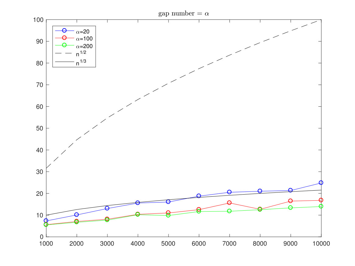 Figure 1
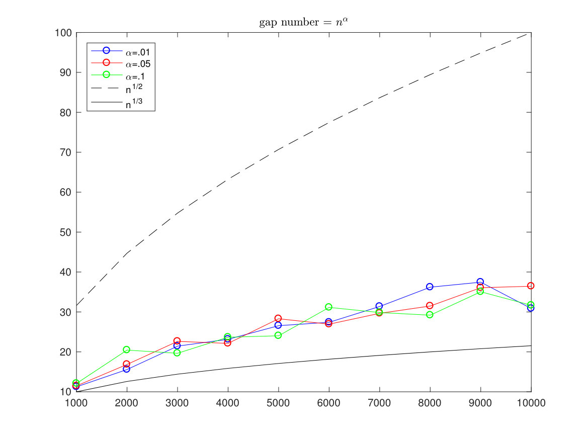 Figure 2
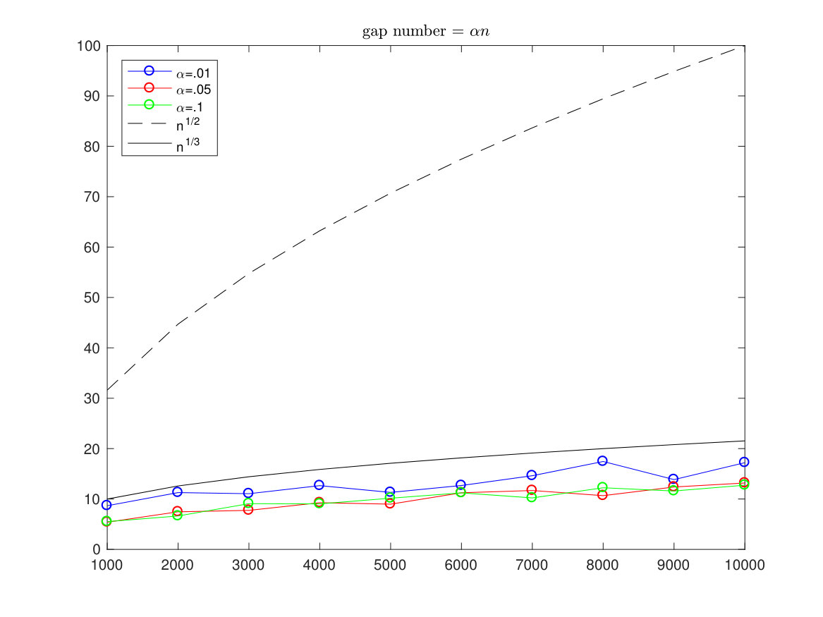 Figure 3
Peer Reviews
No public reviews on file for this paper yet. If you reviewed it on a platform where reviews are public (OpenReview, ICLR, NeurIPS, ICML), you can paste yours below so the community can read it here.
Videos
No videos yet. Explain this paper in a talk, walkthrough, or lecture? Add one.
Non-normal limiting distribution for optimal alignment scores of strings in binary alphabets
Jun Tao Duan
School of Mathematics
Georgia Institute of Technology
Atlanta, GA, 30332
,
Heinrich Matzinger
School of Mathematics
Georgia Institute of Technology
Atlanta, GA, 30332
and
Ionel Popescu
School of Mathematics
Georgia Institute of Technology
Atlanta, GA, 30332
Institute of Mathematics of Romanian Academy
21 Calea Grivitei Street, 010702 Bucharest, Romania
Facultatea de Matematica si Informatica - Universitatea din Bucuresti
Str. Academiei nr.14, sector 1, C.P. 010014, Bucuresti, Romania
Abstract.
We consider two independent binary i.i.d. random strings and of equal length and the optimal alignments according to a symmetric scoring functions only. We decompose the space of scoring functions into five components. Two of these components add a part to the optimal score which does not depend on the alignment and which is asymptotically normal.
We show that when we restrict the number of gaps sufficiently and add them only into one sequence, then the alignment score can be decomposed into a part which is normal and has order and a part which is on a smaller order and tends to a Tracy-Widom distribution. Adding gaps only into one sequence is equivalent to aligning a string with its descendants in case of mutations and deletes. For testing relatedness of strings, the normal part is irrelevant, since it does not depend on the alignment hence it can be safely removed from the test statistic.
1. Introduction
Optimal Alignments are among the main two components used by most DNA-alignment algorithms which try to find similar substrings in DNA-sequences. Because of its great practical importance, these problems have received a tremendous amount of attention.
Let us explain the key points from the DNA perspective. DNA sequencing is one of the most important areas of study in biology. This is still rather expensive and very complex. Suppose now that in a certain animal population, a certain gene is detected. This gene is probably likely to appear in the DNA of other animals too, but in a slightly different form. Thus, instead of repeating the same costly experiments on other animals to find the gene, they just search for a DNA-segment which looks similar to the gene in the first population. This is why often DNA-strings in different animals are compared in order to find places that are related. For more details on the analysis of DNA we refer the reader to [11] and in particular the iid assumption which appears also in this paper is explained on page 14 of the [11].
Here is a more concrete example. Assume is a hypothetical DNA of an ancestor with two descendants, one with the DNA string (which lost the and the ) and another with the DNA equal to (which had an mutated into a ). We align these strings (with gaps), as follows:
[TABLE]
In the analysis of the DNA one has access to the DNA of the descendants only. In terms of the alignments, one is interested in the historic alignment. In our example, we would have that the alignment is given by:
[TABLE]
and we call this the historic alignment. The letters which disappeared in one descendant are now represented by gaps. Which alignment with gaps corresponds to the evolution history of the strings is not known apriori. In other words, in our example, we know the strings and , but not “the true historic” alignment given here by (1.1).
To guess which alignment is historic, the natural attempt is to find an alignment which maximizes similarity. For this, one starts with a scoring function which measures similarity between letters. (Here is the alphabet augmented by one symbol for the gap). The total score of an alignment is then the sum of the scores of the aligned symbol pairs. In alignment (1.1), the alignment score is equal to
[TABLE]
where stands for a gap. An alignment , which for given strings and maximizes the alignment score is called an optimal alignment. The score of an optimal alignment is called optimal alignment score and we will denote it by
[TABLE]
where the maximum above is taken over all alignments with gaps of and .
Which alignment is optimal depends ultimately on the scoring function used. Often, the scoring function biologists work with is a log likelihood. For this, one assumes models of letters evolving independently of their neighboring letters. One takes as scoring function , the logarithm of the probability that an ancestor letter evolves into an in one descendant and into a in the other descendant. Here and are any two letters from the alphabet under consideration, or also the gap symbol. With this choice of scoring function, the optimal alignment becomes the maximum-likelihood estimate for the historic alignment.
A high optimal alignment score indicates relatedness of the two DNA-strings. Thus in testing for relatedness of DNA-strings one usually takes as test statistics the optimal alignment score. The significance of such a test depends then on the order of magnitude of the fluctuation of the optimal alignment score.
It has been a long open question whether for two independent i.i.d. strings of length , the fluctuation of the optimal alignment score is of order or . (See [29] and [9]). In this paper, we think we can see why these two different conjectures co-exist at the same time. We show that for two independent i.i.d strings of length the optimal alignment score (depending on the parameters) can contain a normal component with fluctuation of order . This component is not relevant for finding the optimal alignment score, because it does not depend on the alignment.
When testing for relatedness of DNA-strings one should remove this normal component, since it is only noise. This can be done by modifying the scoring function. Once we “cut out this normal component”, the question that remain is what is the asymptotic distribution of the remainder? Is it Tracy-Widom? We can’t prove it in full generality, however we check this for the special case where the number of gaps is a small power of the length of the strings and the gaps are allowed only into one string.
*We also exhibit a scoring function with an alignment score which is of the order but not normal, nor Tracy-Widom. This, should then show that any claim that the order automatically implies asymptotic normality is wrong! (Here designates the optimal alignment score of two i.i.d. random strings of length .) To prove normality, one needs a more detailed knowledge of the path structure of the optimal alignments! *
The optimal alignment can be viewed as a special case of Last Passage Percolation with correlations. To our knowledge, many of the proofs for models of First and Last Passage Percolation, where the asymptotic distribution is known, go back to proving asymptotic equivalence with the following functional of Brownian motions: Consider a sequence of i.i.d. standard Brownian motions. Also consider when goes to infinity, the functional
[TABLE]
which properly rescaled becomes Tracy-Widom [5, 14, 25]. Now, in our case, we have a similar situation, where instead we have a sequence of dependent identically distributed standard Brownian motions . However, the correlation structure is rather simple. Precisely, there exists a Brownian motion and i.i.d Brownian motions so that
[TABLE]
for all . Hence, instead of independent Brownian motions we have correlated ones and the maximum given in (1.2) can be written as
[TABLE]
Hence, we get a normal component plus a term on a smaller scale which is indeed Tracy-Widom. This is the reason why we can prove in the current paper, under a very special situation (adding gaps only into one string and keeping their number a small power of ), that in the limit we obtain a normal plus Tracy-Widom on a smaller scale. However, the normal part is often irrelevant for the optimal alignment problem.
Note here that the normal component does not dependent on the choice of (which in what follows, correspond to alignments). Again, the normal component is in some sense irrelevant for finding the optimal alignment. We should leave it out because it is only added noise.
1.1. History of this problem
We consider two random i.i.d. strings and . In the sequel, denotes the optimal alignment score of and .
Chvatal-Sankoff proved [9] that converges to a constant , but is not known in most cases. In [15], [16] we have good confidence intervals for . We have been able to prove the order
[TABLE]
in many situations [23],[7], [2], [17]. This proves the conjecture of Waterman [29] (for certain specific distributions of the letters and scoring functions), but is different from what Chavatal-Sankoff have conjectured. The order conjectured by Chavatal-Sankoff is the order which one would expect knowing that is also the weight of the heaviest path from to in an LPP-formulation of our problem. (In the physics literature, [18], the order for the standard deviation of the heaviest path from to in a vast class of LPP-models is conjectured to be not . For more details see also [20]).
Let us explain what LPP is and how our optimal alignment can be formulated as an LPP-problem with correlated weights. In LPP, one considers an oriented graph with a random weight function of the edges. Let . A path from to in the graph is then defined as a sequence of vertices: where and for all . The total weight of the path is given by:
[TABLE]
an optimal path from to is then a path which maximizes the total weight among all paths from to .
Now, our optimal alignment problem can be formulated as an LPP on the integer lattice with the optimal alignment score being the weight of the path of maximal weight from to . For this we take the set of vertices to be and the edges to go always one to the right, one up or diagonally up to the next vertex. The weight for horizontal and vertical edges is minus the gap penalty. For the edge the weight is . With this setting when we align a letter with a gap, this corresponds to moving one unit vertically or horizontally. Aligning with corresponds to moving along the edge . The optimal path then defines an optimal alignment where for every edge contained in the optimal path, aligns with . The transversal fluctuation measures how far the optimal path from to deviates from the diagonal.
Let us give an example. Take the two strings and . Consider the following alignment with gaps:
[TABLE]
We can represent this alignment as a path on the integer points in two dimension. We are always allowed to go to the left by one unit or up by one unit or diagonal to the next integer point. When we go horizontal or vertical, this means that we align a letter with a gap. When we go diagonal this means that we align two letters with each other. Below, we show how we represent the alignment given in (1.3) by a path on the two dimensional integer lattice:
[TABLE]
To visualize, the path represented by the last table above, draw short segments between the points: [math] to , then to , ….and up to a segment from to . The path is then given by this sequence of segments. So, the first such segment from [math] to is diagonal, and corresponds to aligning the two ’s with each other. The score-contribution for this is . Then, the segment from to is diagonal and corresponds to aligning the ’s. Its score contribution is . The segment from to is vertical and hence corresponds to aligning a letter with a gap. In the current case, it is the first in which gets aligned with a gap, and the score for this is the gap penalty . Then is again diagonal and corresponds to aligning with , with score . Then, the segment is horizontal and corresponds to aligning in with a gap, which contributes to minus a gap penalty to the total score. The final segment is diagonal, and corresponds to aligning the last of with the last of . Score is then . In other words, the horizontal or vertical moves contribute minus a gap penalty each, whilst the diagonal moves contribute to the score by aligning the corresponding letters. IN THIS EXAMPLE, WE ALIGNED ONLY IDENTICAL LETTERS. This is not always the case. In DNA-analysis, when letters can mutate we also align similar letters with each other, not just identical.
Formally we can view an alignment with gaps of the strings and as a couple consisting of two increasing integer sequences. The sequence
[TABLE]
and the sequence
[TABLE]
are non-negative integers. Here is any integer non-negative number. The alignment with gaps defined by is then the alignment which aligns with for all and aligns all remaining letters with a gap. The alignment score is then
[TABLE]
where is represents the total gap penalty. (The penalty for one given gap being ). In our current example, we have the number of aligned letter pairs is . Furthermore, we find: , whilst . The path representing the alignment given by is the path containing all the segments:
[TABLE]
for and additionally a minimum amount of vertical and horizontal unit length integer segments so as to make this a connected path.
First Passage Percolation (FPP) and LPP are part of a vast area of statistical physics [18] which is concerned with random growth models for which physicists expect some universality properties. More specifically, one considers growth of a cluster where material is being attached randomly on the surface of a nucleus. There are many fundamental questions open for decades, such as the universality of the fluctuation exponents. Many theoretical physicists, crystallographers and probabilists have worked on this and many conjectures have been formulated [18], as for example that the fluctuation should behave like and the transversal fluctuation should be or order (see KPZ-conjecture in [20]). These are difficult conjectures and rigorous results were obtained only under some special circumstances of LPP models, like Longest Increasing Subsequence [3], LPP on with exponential or geometric waiting times [19] and the case of percolation in a narrow tube [8]. To our knowledge, the best results show only a fluctuations of less than [4] and above [27].
We have been able to prove our results for several Longest Common Subsequence (LCS) and Optimal Alignments (OA) models.
LCS are a special case of OA. For two strings and a common subsequence of and is a sequence which is a subsequence of and at the same time a subsequence of . A LCS of and is a common subsequence of and of maximum length. The length of the LCS of and can be viewed as an optimal alignment score of and . For this we take to be if and otherwise. On top the gap penalty should be taken [math]. With this choice, the length of the LCS is also equal to the optimal alignment score.
Our results together with the results of Baik, Deift and Johansson [3], are among the few rigorous results determining the exact order of the fluctuation exponents for some non-trivial FPP or LPP related 2-D models. In their work, as in ours, the fluctuation is of order and the rescaled asymptotic limiting law is Tracy-Widom. Another interesting paper is for the TASEP model, by Borodin, Ferrari, Praehofer and Sasamoto [1]. There they do not use the same approach of reducing the problem to formula (3.11) and (3.12), and it is not the GUE which appears in the limit, but GOE. Other methods used to establish the solvability of LPP models are the vertex operator and fock space formalism put foward by Okounkov [26] in the study of Schur process.
Our paper is organized as follows. In Section 2, we introduce the main decomposition of the scoring function and show examples where the limiting distribution of the optimal alignment score is normal alongside with other examples which are non-normal. In the next section, namely Section 3, we restrict the number of gaps to a certain number which is finite and fixed and allow the gaps only in one sequence. Here we give a general description of the optimal alignment in terms of multiple dependent random walks and outline an argument which supports the conjecture that under some conditions, if is replaced by with small , then the (rescaled) limiting distribution of the optimal alignment is Tracy-Widom. We can not prove this statement rigorously in general, but in the next section, namely Section 4, we prove this for the key scoring function under the assumption that the number of gaps is for small and the second sequence of letters is distributed normally rather than . The main rigorous result is stated in Theorem 4.1 and appears in Section 4.
Section 5 is dedicated to technical results while the last one, Section 6 contains a few simulations.
2. Linearly decomposing the space of scoring functions
In this section we discuss the general decomposition of the scoring function in a natural basis. The point of this is that some of the scoring functions are in some sense artificial because the optimal score does not depend on the alignment. This will give a normal behavior in the limit for the optimal score.
We consider symmetric scoring for a binary alphabet. We do not allow alignments of gaps with gaps, so the scoring functions we consider are given by a matrix, with one irrelevant entry, namely
[TABLE]
Here stands for a gap. In our case we will put and we will always assume that the above matrix is symmetric hence and , whilst . The linear space of such symmetric matrices is generated by the following five elements
[TABLE]
and
[TABLE]
Note that the matrices , and are orthogonal to each other (with respect to the canonical inner product given by ). Also, the matrices and concern only with the gap penalty. Thus, any scoring function we will consider can be written as
[TABLE]
First, it is important to note that the part gives the same alignment score for any alignment. This is so, because and can both be viewed as linear additive functions in the following way. For a given a function , take the “linear “scoring function defined by:
[TABLE]
for all .
We also assume that . Clearly for such a “linear” scoring function, with value , the alignment score for any alignment does not depend . Indeed, it is trivial to check that
[TABLE]
Furthermore, the expression on the right side of the above equality is a linear function of a binomial random variable. Now, in our case, is of the above type with the function given by
[TABLE]
Thus, we find that
[TABLE]
where denotes the total number of ’s in both strings and combined whilst denotes the number of ’s in both strings combined. Noting that , we finally find that
[TABLE]
Here is a binomial with parameter and , consequently,
[TABLE]
Similarly, the alignment score according to does not depend on the alignment and is also equal to . Since the alignment scores according to and do not depend on the alignment we find for any scoring function that the optimal alignment score can be decomposed as follows:
[TABLE]
According to the central limit theorem, is asymptotically normal on the scale and thus we can conclude that
[TABLE]
where .
Now, since the part does not depend on the alignment it has no affect on which alignment is optimal. Also, it is just noise added for testing if sequences are related or not. This noise can be removed, since it is known. Equivalently, we can just take as scoring function instead of .
2.1. Normal and non-normal cases
In this section we present a simple example for which the optimal alignment score, properly rescaled, converges to a distribution which is not normal. Interestingly, the scaling is still the same as in the case of the previous section, namely, .
As mentioned, for scoring functions of the type , the alignment score does not depend on the alignment of the strings and . Furthermore, the limiting distribution of the optimal alignment score is normal on the scale since
[TABLE]
where is the total number of ’s in the concatenated string . Since is binomial with parameter and , the above optimal score, properly rescaled converges to the normal. Thus we can interpret the scoring function with as degenerate and hence not relevant for practical purposes.
Next we consider the following scoring function
[TABLE]
If designate the number of ’s in and designate the number of ’s in , then, the optimal alignment score according to the scoring function is simply equal to the minimum of and , namely,
[TABLE]
This is so because aligning a with a gives a negative score, whilst aligning something with a gap gives [math]. So, the optimal alignment is going to align all ’s with gaps. Since an aligned with an scores positively, the optimal alignment is going to align a maximum number of ’s with each other.
Note that and have the same expectation and both tend asymptotically to be normal when re-scaled by . Hence, we get
[TABLE]
where and are two standard normal independent of each other, which is certainly not normal. Thus, we have a non-normal limiting distribution, but still we have a fluctuation on a scale !
Notice also the following interesting fact, namely that there are many different alignments, which are very far away from each other. Indeed, say that . Then, the optimal alignments can be characterized as follows. Choose a subset of ’s in with cardinality equal to . These ’s are aligned with gaps. Then align all the remaining ’s in with ’s from . Finally, align all the ’s with gaps.
Now, real life scoring functions should not have too small, since in practical situations, like genetic evolution, there are usually not too many gaps. This reflects the fact that there are not too many deletes from an ancestors DNA. In the next section we show that if we look for the optimal alignment under the constrain of the total number of gaps being small, then we get that can be decomposed into a normal part on the scale plus a smaller part whose limiting distribution is non-normal.
3. Fixing the number of gaps and allowing them only in one
sequence
In this section, under the assumptions that the number of gaps is finite and fixed, we present a general outline of an argument which should be sufficiently convincing that the limiting behavior of the optimal alignment is normal in the scale plus a Tracy-Widom on a smaller scale.
Let us assume that we only consider alignments with a fixed number of gaps equal to , where is a fixed constant. To simplify the problem we will allow the gaps only in one sequence.
Let be a constant and let and be the two random strings of letters. Thus, we will align exactly letters from with gaps, but all the letters of will be aligned with letters of . We will consider the optimal alignment of and under the constrain that there are exactly gaps all inserted in . The corresponding optimal score will be denoted by . To specify an alignment we simply need to specify which letters of get aligned with gaps, thus we need to specify a sequence of increasing integers . The vectors consisting of these integers then define our alignment, namely, align with a gap for all .
Let denote the random walk defined recurrently on by
[TABLE]
and then:
[TABLE]
for all and for . (To simplify the notation we assume that the sequence of the ’s is a double infinite sequence of i.i.d. variables
[TABLE]
In the problem which we will consider only a finite number of ’s will have and their contribution will be negligible).
For example, the first random walk is then defined by
[TABLE]
Similary, the second random walk is defined as follows:
[TABLE]
Consider the alignment score under the constrain that the -th gap is aligned with , for all , where is a given increasing sequence of integers. The alignment with exactly gaps is uniquely defined by this constrain and its alignment score is:
[TABLE]
Recall that we assume a zero gap penalty.
Let us give an example. Take the string and we could align and with a gap. Then we have gaps and whilst . So, this defines the -gap-alignment given by:
[TABLE]
Hence, the alignment score with a [math]-gap penalty is equal to:
[TABLE]
Let us denote by the optimal alignment score under the constrain that the alignment contains exactly gaps all aligned with letters from . Since the gap penalty is [math] the formula for is then given by
[TABLE]
Hence, the maximum is obtained by choosing the increasing sequence which maximizes the following sum:
take the increment of the first random walk on , then we add the increment of the second random walk on and keep on going until the increment of the last random walk on has been added.
Next, we are going to put the different one-dimensional random walks together into one vector:
[TABLE]
In this manner becomes a -dimensional ”correlated” random walk. Thus we have and
[TABLE]
If we subtract the drift and rescale by , the multidimensional correlated random walk converges to a dimensional Brownian motion and we refer to [21, 22] for more details. This means, that holding fixed, we can find a which goes to [math] as goes to infinity so that there exists a -dimensional Brownian motion for which
[TABLE]
holds with probability where goes to [math] as . Here the Brownian motion depends on , but of course, its distribution does not. If is not an integer then we take for the linear interpolation of . Let us introduce a small modification of . This modification will be denoted by and is equal to
[TABLE]
Clearly with this definition,
[TABLE]
where Note that for all the random walks , the drift is the same and equal to . Now, we can rewrite using the unbiased random walk
[TABLE]
Assume next that inequality (3.2) holds. Then, we can approximate the unbiased random walks on the right side of (3.4) by components of a Brownian motion according to (3.2). Since the sum contains terms, the approximation error will be at most (if we assume (3.2) to hold) and thus
[TABLE]
where refers to the maximum
[TABLE]
We can now use inequality (3.5) together with (3.3) to find
[TABLE]
The component of our Brownian motions could be correlated. To see this, let’s calculate the covariance between the first two random walks, that is between and . The idea is that most terms of the sum corresponding to the random walk are not correlated, however the closer ones are correlated. To the point, take for example the first term in the sum
[TABLE]
Since, the ’s and ’s are all independent of each other, an expression of the type can only be correlated with if either or . Therefore, in the sum
[TABLE]
there are only two terms which can have non-zero correlation to . These terms are and . This analysis holds true for every term in the sum for the first random walk. Only in the very last term in the sum on the right side of (3.7) there is a term for which there are not two terms in the sum on the right side of (3.8) correlated with it. Hence, the covariance between (3.7) and (3.8) is about times constant, where the constant is given as the covariance between and .
Let us expand on this calculation a little bit by looking at the covariance terms
[TABLE]
We can work out the same calculation for all pairs of random walks and provided . The covariance is always about . Hence, the multi-dimensional Brownian motion in our approximation (3.2) has a covariance matrix with all non-diagonal entries equal to . Hence, we find
[TABLE]
for and
[TABLE]
This is a simple covariance structure since there is one common factor contained in all the Brownian motions if is non-zero. In other words, we find that there exists a multidimensional Brownian motion with all components independent and having variance
[TABLE]
so that
[TABLE]
where represents the -dimensional identity matrix and is a one dimensional Brownian motion which is independent of . (To understand more in detail how we get the and the consider this: simply take a Brownian motion with [math] expectation starting at [math] and independently a collection of Brownian motions which among themselves are i.i.d. Also, the ’s have all [math] expectation and start at [math]. You can now chose all these Brownian motion, so that have the same correlation structure then the collection . Then, because you deal with gaussian process you have the same distribution. Then you can make a perfect coupling between the and the since they have the same distribution). We also have
[TABLE]
Hence, we find that
[TABLE]
where
[TABLE]
It is known (see [5, 14, 25]), that the rescaled goes asymptotically to Tracy-Widom, more precisely,
[TABLE]
where convergence is in law as . Hence, there is a sequence of random variable which goes to [math] in probability as , and a sequence of variables each having same Tracy-Widom distribution, so that
[TABLE]
We can now rewrite expression (3.6) using (3.10) and get
[TABLE]
which, with the help of equation (3.13), becomes
[TABLE]
For the above inequality to be useful, we need the right side of it to be smaller than . This will depend on the value of . Now, we want to let go to infinity at a slower rate then . Most papers on closeness of random walk and Brownian motion are for fixed dimension. Also, in our case, any consecutive components of the multi-dimensional random walk are correlated. However, still assuming that the approximations hold for fixed dimension and correlated multidimensional random walk, we could take to be
[TABLE]
whilst
[TABLE]
for a constant not depending on or . In this case for the inequality (3.15) to be useful, we would need
[TABLE]
to be of smaller order than . This is the case when , with small enough.
4. Letting the number of gaps and normal letters
In this section, we are going to treat the case where the number of gaps increases to infinity with and the simplest such scenario is the case of
[TABLE]
for some small which we assume is not depending on . Again, we look for the best alignment score under all alignments with the prescribed number of gaps being and the gaps appear only in the sequence of ’s, thus we allow gaps to align with ’s.
The highest alignment score among all alignments which align exactly letters of with gaps, but no letter of with gaps, is again denoted by
[TABLE]
When the number of gaps is fixed, in determining which alignment is optimal, the penalty for gaps does not matter much. Indeed, the gap penalty will affect the optimal alignment only by a term of order . Moreover, if we assume that the penalty of aligning a letter with a gap does not depend on the letter, we can simply assume that the gap penalty is actually equal to [math].
Therefore, the only part of the scoring functions which matters is the symmetric matrix
[TABLE]
The space of all such symmetric matrices constitute a dimensional space where a basis is formed by the matrices
[TABLE]
In addition, if we define two scoring matrices to be equivalent if the optimal alignments are the same, then it is easy to see that for any arbitrary scoring function , the scoring itself and are equivalent. Thus the main task is to understand what happens under alignments with the scoring function . Thus we assume for the rest of the section that the scoring function is equal to , so that:
[TABLE]
Now, in the case considered here of a two dimensional alphabet, that scoring function can be viewed as a product scoring function by observing that if we introduce a numeric code for the letters, namely take to be and to be . Then we find that
[TABLE]
Using this in (3.10), the key observation is that the part has covariance given in formula (3.9) by
[TABLE]
which in the present case becomes
[TABLE]
due to independence and mean [math] of . Hence, the term disappears from inequality (3.15) for this choice of the scoring function.
Next, we notice that for a one dimensional “uncorrelated” random walk, the best coupling of the walk with a Brownian motion in (3.2) can be attained with (see [22]).
With this choice of , the term in (3.15) is of order , thus is much smaller than which is of order . However, since we have to correlate a large number of random walks (exactly and not independent), we expect to be larger than .
A different look at the dominating term on the right hand side of (3.15), gives that
[TABLE]
which is enough (at least heuristically) to guarantee that the rescaled optimal score is asymptotically Tracy-Widom.
In order to deal with the approximation of the random walk by Brownian motions, we need to get good couplings of the random walk with Brownian motions. This is what we want to do next.
We should also quickly mention, that at this stage, it should be heuristically clear why we should expect Tracy-Widom as limiting distribution as soon as the constant is small enough. Indeed, when is very small, then should be as “close as we want” to the formula for the one dimensional random walk with independent increments. Now, for the one-dimensional random walk, it is known to allow a coupling to a Brownian motion with . Again, the only problem is to find a good coupling of the multidimensional random walk to a multidimensional Brownian motion. The random walk has components. Furthermore, there is dependency among the increments of the random walk. Each step (increment) of the random walk, can depend on steps before and after. Hence, is independent of for all .
The main question is thus how well can a random walk with dependencies be approximated by Brownian motion? (See [21, 22] for the one dimensional case, [12] for severeal dimensions and [24, 10] for overviews.)
Is it possible to find such a coupling when the dimension of the random walk grows to infinity? This is delicate as the constants involved depend on the dimension and thus are not very useful in our case.
Unfortunately we can not treat both problems simultaneously and it seems highly technical to deduce such a result in great generality. Instead, we present here a simple approach for a simplified situation.
First, we use the fact that our scoring function is a product. Furthermore, for the rest of the paper we also assume the variables to be i.i.d. normal with
[TABLE]
instead of binary variables. The variables are still binary variables in this section with
Again, since the component in the equation (3.15) dissapears.
The normal assumption on ’s is in place here to simplify the calculations. We believe that macroscopically it amounts to the same as taking these variables binary. The fact that the variables are standard normal instead of binary has a very important consequence on the calculation side, namely, the optimal alignment still tries to align the maximum number of letter with the same sign and also will try to get that those ’s which get aligned with an of opposite sign to be small in absolute value.
The key strategy of the proof is to condition on the sequence and exploit the normal structure of the . To set up the ground, let and let be a non-random binary vector. We are going to work conditional on .
Now, consider our random walk in the current case where . We have
[TABLE]
where and
[TABLE]
Looking at the above expression for the random walk , we see that the steps are dependent but once we condition the ’s to be constants, i.e. and to be i.i.d , the ’s become independent normal vectors. Hence, conditional on , we get that the multidimensional random walk has independent normal increment with expectation [math].
This random walk is not yet a Brownian motion restricted to discrete times but we are going to show that we can construct such a Brownian motion which is a good approximation. In order to do this we consider at first the random walk restricted to the times which are a multiple of
[TABLE]
with some small which will be determined later and denoting the integer part of .
Thus, we will consider
[TABLE]
where to simplify notation we assume to be a multiple of , though we can formally replace by with and run essentially the same argument.
Using the independence of the increments conditional on , we calculate the covariance matrix of the position of the random walk at time in the following way:
[TABLE]
The key fact here is that with very high probability the last sum in the above equation is approximately where is the identity matrix.
Now, using this, and the fact that is the covariance matrix of a standard -dimensional Brownian motion at time we will show that there is a coupling between the random walk and a standard Brownian motion such that is close to the Brownian motion position at time . Moreover the argument can be extended to include also the increments of the random walk. More precisely, we show that the coupling can be chosen such that the increments
[TABLE]
are also close to the increment of the coupled Brownian motion.
To construct such a coupling, we will build a Brownian motion
[TABLE]
by coupling at the times at first. More precisely, we couple with , then the increment with the increment and then we continue coupling the next increment with and so on and each step we do this independently of the construction at the previous steps. Recall that we do this conditionally on .
The key is that the construction at each step is a consequence of Lemma 5.1 in the next Section 5.1 where we show how to couple a normal random variable having covariance close to a multiple of the identity. Essentially the main assertion here is that if is a normal vector such that
[TABLE]
then we can find a normal vector of i.i.d normal components such that . Here we use the operator norm for a matrix and measure the closeness in the operator norm, in particular all components of have variance at most .
Once all the increments are defined, we define for as the sum
[TABLE]
Conditional on , the pieces
[TABLE]
for are independent. Since
[TABLE]
depend only on (4.9), this implies that conditional on , the sequence of random vectors
[TABLE]
constitutes a multidimensional standard Brownian motion restricted to the times . We can for instance use the construction of Levy for the Brownian motion to extend these vectors to a Brownian motion such that the increments are given exactly by for . We do not look for other details about the Brownian motion during the times , we will simply use some basic estimates for the maximum of Brownian motions between these time intervals. For instance using the reflection principle we can show that
[TABLE]
In particular what this yields is that for some constant independent of and
[TABLE]
thus the deviation of the Brownian motion on each of these intervals is very well controlled.
Now define a few events related to our coupling which will take care of the main estimates.
- •
Let be the event that none of the components of the standard multidimensional Brownian motions goes further than during any of the time intervals for That is let be the event that
[TABLE]
for all . Set
[TABLE]
- •
Let be the event that the multidimensional random walk does not move further than during any of the time intervals . Hence, let be the event
[TABLE]
for all . Let
[TABLE]
- •
The event takes care of the fact that the covariance matrix of for all is close to ,were denotes the identity matrix. More specifically, let thus be the event that
[TABLE]
where is a constant which will be defined later. Similarly for any integer so that
[TABLE]
holds, let be the event that
[TABLE]
Finally let be the event
[TABLE]
- •
The next event assures that the random walk and the Brownian motion are close to each other at times which are multiples of . More specifically, let be the event that the -th component of at times which are multiples of is bounded as follows:
[TABLE]
Let be intersection of these for all , precisely:
[TABLE]
Now, we summarize the picture we have obtained so far. Rescale the random walk and the Brownian motion by a factor and the time by a factor by setting for
[TABLE]
By scaling the Brownian motion, we know that is again a Brownian motion. When the events , and all hold, inequality (3.2) is satisfied for the multi-dimensional Brownian motion with given as
[TABLE]
where again, the number of gaps and the time step are given by
[TABLE]
We can now go back to inequality 3.15, to find that:
[TABLE]
holds with probability at least where
[TABLE]
Recall also, that designates a sequence of random variables which go to [math] in probability. The sequence designates on the other hand a sequence of random variables which are all identically distributed according to Tracy-Widom.
We eliminated the term by increasing the coefficient in front of .
Furthermore, from inequality 4.12, we obtain the important conclusion that in order to show that the re-scaled optimal alignment score with imposed gaps goes to Tracy Widom we only need to prove prove two things:
I: goes to zero, hence
[TABLE]
as , which we solve in Section 5.2.
II: The term
[TABLE]
in the bound in 4.12 is of order less than . This is the place where we choose and .
We have to verify that there exists a choice and making expression 4.15 less than order . In other words, we want
[TABLE]
which is satisfied for large enough as soon as
[TABLE]
This is of course possible if and only if
[TABLE]
which leads to . Thus, for any , we have convergence of the re-scaled optimal alignment score to Tracy-Widom. Hence, we are able to prove our result provided there are less than order gaps in the optimal alignment! Let us formulate this fact in the form of a Theorem.
Theorem 4.1**.**
Let be a constant. Let be an i.i.d. sequence of binary variables so that
[TABLE]
and let be an i.i.d. sequence of standard normal random variables. Let denote the scoring function defined by for any two letters of our binary-alphabet. Let . Then, the optimal alignment score with constrain to have gaps and properly rescaled as
[TABLE]
converges in law to Tracy-Widom.
Proof.
Multiplying (4.12) by , we find that that
[TABLE]
holds with probability at least , In the next section it is proven that goes to [math] as . (Recall also inequality (4.14)). Furthermore, since , we have from (4.16) that
[TABLE]
goes to [math] as . Hence, since also go to [math] in probability, we have that
[TABLE]
goes to [math] in probability, when . Hence, since always has Tracy-Widom distribution, it follows, that
[TABLE]
converges in Law to Tracy-Widom as . But, when we replace by in expression 4.20, we obtain expression (4.17) from our theorem. So, we just finished proving that (4.17) converges to Tracy-Widom in Law. ∎
Remark. We believe that taking the variables binary instead of standard normal our theorem should holds for small enough. However, the proof for approximating the multidimensional random walk by a multidimensional Brownian motion will be much more difficult. The intricate part is very similar to passing from the CLT to Berry-Essen type CLT theorem is when there are non-finite correlations or dimension goes to infinity at the same time as (see [6], [13]).
Now we got Tracy-Widom limiting distribution for the binary case, by using the scoring function and fixing the number of gaps. If instead we use a scoring function
[TABLE]
then we get an additional normal term on the scale . Indeed, and do not affect which alignment is optimal, thus,
[TABLE]
As argued before, depends only on the number of ’s and ’s in each of the sequences and . It is even a linear functional of these numbers of occurrences and hence asymptotically normal on the scale . On, the other hand, according to our theorem, we have that after rescaling is asymptotically Tracy-Widom on the scale , (provided and ). Thus, there is a larger normal part and Tracy-Widom on a lower scale. But, for optimal alignment of DNA sequences, one should always set , since the part does not influence which alignment is optimal. In that case when , the limiting distribution is purely Tracy-Widom.
*The main question to ask here is what happens if we allow the number of gaps to be of order which we leave as an open problem here. *
5. Technical results
5.1. How to couple normal random vectors with close
covariance matrix
The main coupling result is contained in the following Lemma.
Lemma 5.1**.**
Let be a -dimensional normal random vector with expectation [math]. Let and . Assume that
[TABLE]
Then there exists a -dimensional normal random vector with covariance matrix and expectation [math] so that
[TABLE]
In particular all the components of have variance at most .
Proof.
The main idea is to construct a normal vector simply by rescaling the vector . The construction uses the fact that if is a linear transformation from into itself, then is again a normal random variable of covariance matrix . In this framework we take and
[TABLE]
Clearly, we now have
[TABLE]
Furthermore,
[TABLE]
Taking the eigenvalues of to be , the condition (5.1) reads as
[TABLE]
On the other hand since , we also know have that . Thus the conclusion is reached from the fact that the eigenvalues of are and the following chain of inequalities
[TABLE]
∎
5.2. Proof that the events , , and all
have high probability
Lemma 5.2**.**
We have that has probability close to one. More precisely, assuming , then for any constant , the following holds
[TABLE]
Proof.
Consider the sum on the right side of (4.2). Instead of taking the full sum, we are going to split the sum in the following form
[TABLE]
where for simplicity we assume that is a lot larger than and that is a multiple of .
Since for each , the sequence
[TABLE]
are iid when runs from to . The covariance matrix of these vectors is the -dimensional identity matrix . So,
[TABLE]
is an estimate of the covariance matrix of . Hence, expression 5.2 is approximately equal to and
[TABLE]
Now, according to [28] the precision of such an approximation in operator norm is the square root of the dimension times the square root of the sample size. More precisely, we have
[TABLE]
Here, is a constant which does not depend on . Hence, for the full sum, this means
[TABLE]
So, we have proven that
[TABLE]
Hence, since and since
[TABLE]
we have
[TABLE]
Since, and with it follows that the dominant term in the bound on the right side of 5.4 is which is an exponential decaying function in a fractional power of .
∎
The next lemma shows that when the event holds, then has high probability
Lemma 5.3**.**
We have that
[TABLE]
In particular, .
Proof.
We work conditional on . We have that when the event holds, then
[TABLE]
where is a dimensional identity matrix. So, our coupling of to is such that the covariance matrix of the difference has norm at most . Thus, conditional on , and assuming holds, we get
[TABLE]
for all . This implies that the -th component of the difference
[TABLE]
has a variance less or equal to . But conditional on , we have that the differences (5.5) are normal, independent with expectation . Taking the -th component of
[TABLE]
at the times is thus like taking a standard Brownian motion at the times where
[TABLE]
Since the variance increases at each step by at most , we get that
[TABLE]
So, the maximum of the -th component of the difference restricted to the times is thus stochastically bounded by the maximum of a standard Brownian motion during the time interval
[TABLE]
The standard Brownian motion starting at the origin. By the reflection principle for Brownian motion, this distribution function can be bounded by the distribution function of the standard Brownian motion at time
[TABLE]
We have just shown that conditional on and when holds, then
[TABLE]
where the last inequality was obtained by using the lemma 5.6 below. We have just proven that
[TABLE]
∎
Lemma 5.4**.**
We have that for all large enough.
Proof.
Let be the event that:
[TABLE]
So, we have
[TABLE]
where designates a standard Brownian motion starting at the origin in a one dimensional space. By the reflection principle, we get that the right side of 5.6 is equal to
[TABLE]
where designates a standard normal. Using Lemma 5.6, we find that the right side of 5.7 can be bounded by so that
[TABLE]
Now
[TABLE]
where in the last interesection above ranges over and ranges over . Hence, we get
[TABLE]
where the dominant term is which beats any power of . Note that is just a power of . ∎
Lemma 5.5**.**
We have that for all large enough.
Proof.
Same as for . So we leave it to the reader.
∎
Lemma 5.6**.**
Let be a standard normal. Let . Then, we have
[TABLE]
6. Simulations
In the pictures below we have simulated the optimal alignment with length running from to and each time we compute the estimated standard deviation (of 100 simulations from a sequence). The gaps are allowed only in one sequence and the number of gaps is restricted to be either a fixed number, a number or a proportional number to .
7. Acknowledgements
We want to thank the reviewers of this paper for the comments which improved the paper.
The reference list from the paper itself. Each links out to its DOI / PubMed record.
- 1[1] Michael Prahofer Alexei Borodin and Tomohiro Sasamoto. Fluctuation properties of the tasep with periodic initial configuration. J. Stat. Phys. , 129:1055–1080, 2007.
- 2[2] Saba Amsalu, Raphael Hauser, and Heinrich Matzinger. Montecarlo approach to the fluctuation problem for lcs and optimal alignments. Accepted in 4th issue of Markov Processes and Related Fields , 2013.
- 3[3] Jinho Baik, Percy Deift, and Kurt Johansson. On the distribution of the length of the longest increasing subsequence of random permutations. J. Amer. Math. Soc. , 12(4):1119–1178, 1999.
- 4[4] I Banjamini, G Kalai, and O Schramm. First passage percolation has sublinear distance variance. Annals of Probability , 31(4):1970–1978, 2003.
- 5[5] Yu. Baryshnikov. GU Es and queues. Probab. Theory Related Fields , 119(2):256–274, 2001.
- 6[6] V. Yu. Bentkus. Lower bounds for the rate of convergence in the central limit theorem in Banach spaces. Litovsk. Mat. Sb. , 25(4):10–21, 1985.
- 7[7] Federico Bonetto and Heinrich Matzinger. Fluctuations of the longest common subsequence in the case of 2- and 3-letter alphabets. Latin American Journal of Probability and Mathematics , 2:195–216, 2006.
- 8[8] Sourav Chatterjee and Partha S. Dey. Central limit theorem for first-passage percolation time across thin cylinders. Probab. Theory Related Fields , 156(3-4):613–663, 2013.