
TL;DR
This paper models branes as points in a dynamic infinite-dimensional space, linking classical and quantum descriptions, and introduces a Stueckelberg-like field to address quantum position operator issues.
Contribution
It develops a novel formalism describing branes as points in a dynamical brane space, unifying classical and quantum perspectives, and introduces Stueckelberg fields to resolve quantum operator challenges.
Findings
Branes can be represented as points in a dynamical infinite-dimensional space.
Quantization of flat branes yields non-interacting quantum fields.
A Stueckelberg-like field is introduced to address quantum position operator issues.
Abstract
It is shown that the Dirac-Nambu-Goto brane can be described as a point particle in an infinite dimensional space with a particular metric. This can be considered as a special case of a general theory in which branes are points in the brane space , whose metric is dynamical, just like in general relativity. Such a brane theory, amongst others, includes the flat brane space, whose metric is the infinite dimensional analog of the Minkowski space metric . A brane living in the latter space will be called "flat brane"; it is like a bunch of non-interacting point particles. Quantization of the latter system leads to a system of non-interacting quantum fields. Interactions can be included if we consider a non trivial metric in the space of fields. Then the effective classical brane is no longer a flat brane. For a particular choice of the metric in the field space we…
Click any figure to enlarge with its caption.
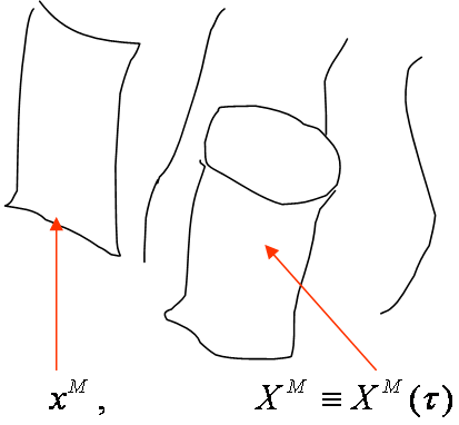 Figure 1
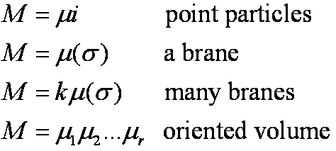 Figure 2
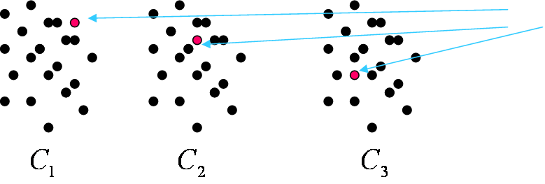 Figure 3
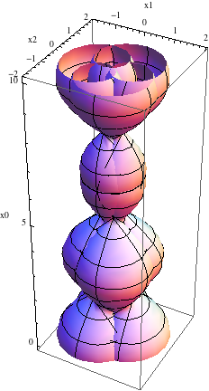 Figure 4
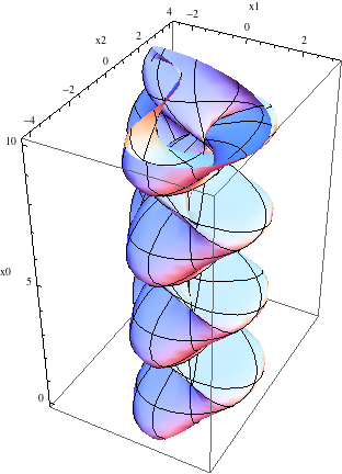 Figure 5
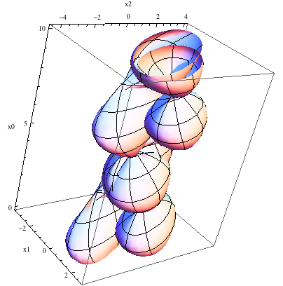 Figure 6
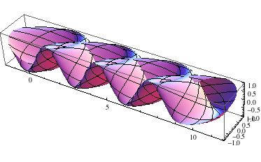 Figure 7
 Figure 8
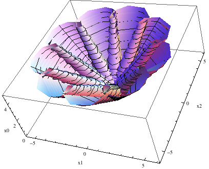 Figure 9
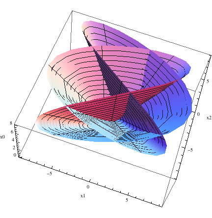 Figure 10
 Figure 11
 Figure 12
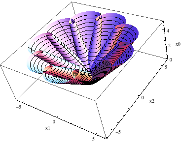 Figure 13
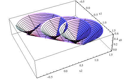 Figure 14
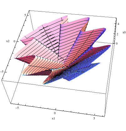 Figure 15
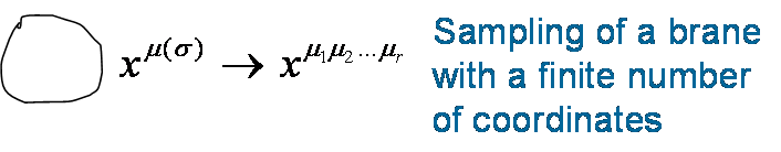 Figure 16
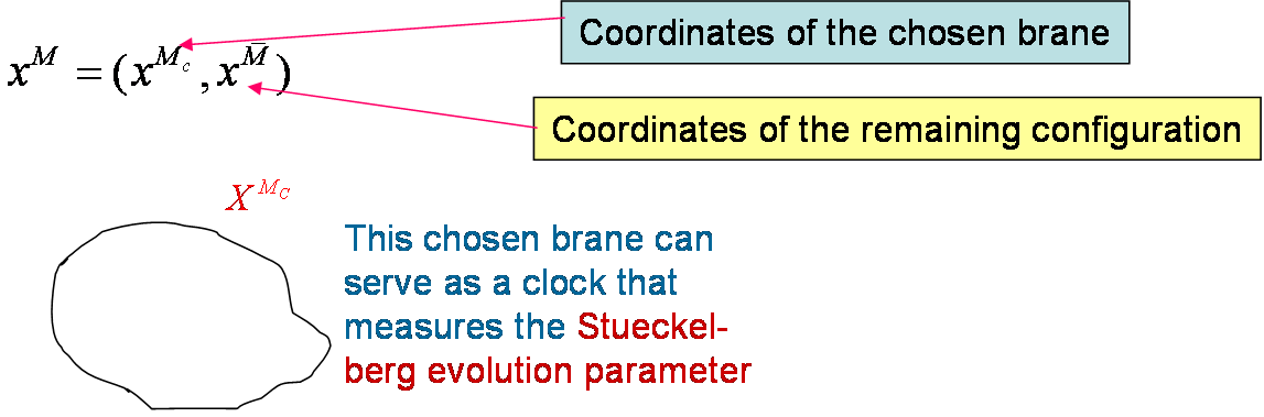 Figure 17
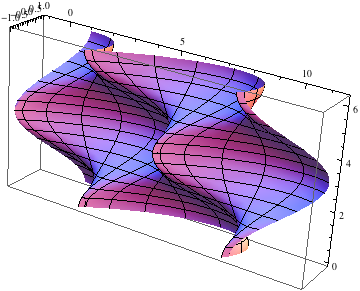 Figure 18
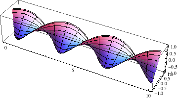 Figure 19
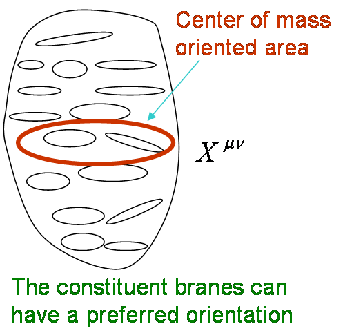 Figure 20
Peer Reviews
No public reviews on file for this paper yet. If you reviewed it on a platform where reviews are public (OpenReview, ICLR, NeurIPS, ICML), you can paste yours below so the community can read it here.
Videos
No videos yet. Explain this paper in a talk, walkthrough, or lecture? Add one.
Branes and Quantized Fields
Matej Pavšič
Jožef Stefan Institute, Jamova 39, 1000 Ljubljana, Slovenia
e-mail: [email protected]
Abstract
It is shown that the Dirac-Nambu-Goto brane can be described as a point particle in an infinite dimensional space with a particular metric. This can be considered as a special case of a general theory in which branes are points in the brane space , whose metric is dynamical, just like in general relativity. Such a brane theory, amongst others, includes the flat brane space, whose metric is the infinite dimensional analog of the Minkowski space metric . A brane living in the latter space will be called “flat brane”; it is like a bunch of non-interacting point particles. Quantization of the latter system leads to a system of non-interacting quantum fields. Interactions can be included if we consider a non trivial metric in the space of fields. Then the effective classical brane is no longer a flat brane. For a particular choice of the metric in the field space we obtain the Dirac-Nambu-Goto brane. We also show how a Stueckelberg-like quantum field arises within the brane space formalism. With the Stueckelberg fields, we avoid certain well-known intricacies, especially those related to the position operator that is needed in our construction of effective classical branes from the systems of quantum fields.
1 Introduction
Relativistic membranes of arbitrary dimension (branes) [2]–[5], are very important objects in theoretical physics. An attractive possibility is a brane world scenario [6]–[27] in which our spacetime is a 4-dimensional surface embedded in a higher dimensions space. Quantization of gravity could then be achieved by quantizing the brane. Unfortunately, quantization of the Dirac-Nambu-Goto brane, satisfying the minimal surface action principle, is a tough problem that has not yet been solved in general. Although the quantization of the string, an extended object whose worldsheet has two dimensions, is rather well understood [28]–[30], this is not so in the case of branes with higher dimensional worldsheets (also called “worldvolumes”).
We will show how to solve this problem by considering the brane as a point in an infinite-dimensional brane space that in general can be curved. The idea is that the metric of is dynamical, just like in general relativity [24, 31, 32]. In particular the metric of can be such that it gives the Dirac-Nambu-Goto brane, which is just the usual “minimal surface” brane. For other choices of -space metric we have branes that differ from the Dirac-Nambu-Goto brane, i.e., they do not satisfy the minimal surface action principle, but some other action principle. In particular, the -space metric can be “flat”, which means that at any point of it can be cast into the diagonal form. Then we have a brane analogue of a point particle in flat spacetime. Such a brane, from now on called flat brane, sweeps a worldsheet that is a bunch of straight worldlines (Fig. 1).
A flat brane is thus just like continuous system of point particles. Quantization of a flat brane then leads to a system of non interacting quantum fields, . The index distinguishes one field from another, and because in the classical theory we had a continuous set of point particles, must be continuous. If we consider interactions among the quantum fields, , then the effective classical theory gives a brane living in a curved brane space, which, in particular, can be the Dirac-Nambu-Goto brane [32].
Instead of one brane a system can consist of many branes. Within the framework of such an enlarged configuration space it is possible to formulate the Stueckelberg quantum field theory with an invariant evolution parameter. We show how the latter parameter is embedded in the system’s configuration.
Each of those branes can be described with a finite number of degrees of freedom, namely, with the center of mass, and additional degrees of freedom that take into account finite extension of the brane. Such extra degrees of freedom can be the coordinates of the Clifford space [33]–[40] that includes scalars, oriented lengths, areas, volumes and 4- volumes (pseudoscalars). In describing a multi brane system we can choose one brane and sample it with the coordinates of Clifford space, while for the remaining branes we retain the description with embedding functions. Clifford space is a 16-dimensional ultrahyperbolic space with neutral signature (8,8). From the scalar and pseudoscalar coordinates that span a 2-dimensional subspace with signature , we can form, with a suitable superposition, the analog of the light cone coordinates. In ultrahyperbolic spaces the Cauchy problem in general cannot be well posed, unless we determine initial data on the “light cone”. In such a way we obtain the generalized Stueckelberg description [41]–[52], [24] of particles and branes, both classical and quantum. The Stueckelberg theory is based on the introduction of an evolution parameter , which is invariant under Lorentz transformations. In the literature we can find various explanations about the physical origin of , but none is generally accepted. In the approach pursued in this and in a series of previous papers [24, 51], the evolution parameter is a superposition of the scalar and pseudoscalar coordinate of the Clifford space, and is thus embedded in the configuration of the chosen brane. The latter brane, which in fact need not be just a brane, but whatever extended object that can be sampled as a brane, thus serves as a clock with which we measure the motion of the remaining branes that form the considered system.
2 Brane as a point in the brane space
The Dirac-Nambu-Goto brane is described by the minimal surface action
[TABLE]
where , is the determinant of the worldsheet embedding functions , , .
An equivalent action is the Schild action [53]
[TABLE]
from which as a consequence of equations of motion we obtain
[TABLE]
The determinant of the induced metric is thus a constant whose choice determines a gauge. We will choose a gauge such that
[TABLE]
in which case the canonical momentum derived from the action (1) coincides with the canonical momentum derived from the action (2). Additionally, we can choose a gauge so that the determinant factorizes according to
[TABLE]
where , , and , , the worldsheet parameters being split as . Then instead of (2) we have
[TABLE]
which can be written as
[TABLE]
which is the -integral of a quadratic form in an infinite dimensional space with the metric
[TABLE]
At this point it is convenient to introduce a compact notation
[TABLE]
and write [32]
[TABLE]
Here we use the generalization of Einstein’s summation convention, so that not only summation over the repeated indices , but also the integration over the repeated continuous indices , is assumed. Indices are lowered and raised, respectively, by and its inverse . The infinite dimensional space is called brane space, because its points represent kinematically possible branes [24, 31].
The quadratic form is invariant under diffeomorphisms in the brane space . A curve in is given by the parametric equation
[TABLE]
where are -dependent functions. The velocity of a “point particle” in is .
The canonical momentum belonging to the action (10) is
[TABLE]
Its contravariant components are
[TABLE]
where .
The canonical momentum associated with the action (6) is
[TABLE]
where we have taken into account
[TABLE]
which follows from (4) and (5). Using the latter equation (15), we verify, that both momenta, (12) and (14), are equal, as they should be. In our notation , whereas is given by Eq. (13).
The momentum satisfies the following constraint:
[TABLE]
We can also form the quadratic form of the momenta in -space,
[TABLE]
in which the integration over repeated indices and is assumed. Comparing (17) and (16), we obtain
[TABLE]
Let us introduce the quantity
[TABLE]
and take into account that Eqs. (18) and (19) imply , i.e.,
[TABLE]
Then we can write the Schild action (10) in terms of the quantities and :
[TABLE]
The latter action is just a gauge fixed action obtained from the action [24, 31, 32]
[TABLE]
which gives a minimal length worldline, i.e., a geodesic in -space. Indeed, the equations of motion derived from the action are [32]
[TABLE]
where
[TABLE]
We use the following notation for functional derivatives:
[TABLE]
Using , and introducing the connection in ,
[TABLE]
we can write Eq. (23) in the form
[TABLE]
which is the equation of geodesic in . If we insert into the latter equation the metric (8), then we obtain the equation of motion for the Dirac-Nambu-Goto brane. Equivalently, if we insert the metric (8) into the action (22) we obtain
[TABLE]
where the Lagrangian
[TABLE]
is a functional of infinite dimensional velocities and coordinates. From the Euler-Lagrange equations
[TABLE]
we obtain
[TABLE]
where . Inserting Eq. (20) into the latter equation, we obtain
[TABLE]
The same equation follows from the Dirac-Nambu-Goto action (1) in a gauge (5).
We have arrived at the minimal length action (22) by using a particular metric (8). However, once we have such an action, we can assume that the metric need not be of that particular form. We can generalize the validity of the action (22) and the corresponding geodesic equation to any metric. In fact, we can assume that the metric of is dynamical, like in general relativity, and that to the action (22) we have to add a kinetic term for the metric . An approach along such lines was investigated in Ref. [24]. Within such a generalized theory the metric (8), leading to the usual Dirac-Nambu-Goto brane is just one of many other possible metrics, including the metric that is the brane space analog of the flat spacetime metric .
3 Special case: flat brane space
The brane theory simplifies significantly if into the action (22) we plug the metric
[TABLE]
Then we have [32]
[TABLE]
This is like an action for a point particle in a flat background space,
[TABLE]
but the background space is now infinite dimensional. Variation of (34) gives the following equations of motion
[TABLE]
where now we have . Choosing a gauge in which , we obtain the following simple equations of motion:
[TABLE]
whose solution is
[TABLE]
This describes a bunch of straight worldlines that altogether form a special kind of brane’s worldsheet, namely a worldsheet of a “flat brane”. Equation (38) thus describes a continuum limit of a system of non-interacting point particles, tracing straight worldlines.
In Fig. 2 we give examples of flat 1-branes (i.e., strings) for various solutions of Eq. (38), i.e., for various choices of . In Fig. 3 we illustrate how the situation looks in the case of a metric that differs from (33). For comparison, in Fig. 4 we show two examples of the usual Nambu-Goto strings.
We see that flat branes can form involved self intersecting objects in spacetime. In the last example in Fig. 2 the worldsheet does not self intersect, which is a consequence of suitable boundary conditions.
Quantization of the system described by the action (34) can be performed in analogous way as the quantization of the point particle, described by (35).
In the case of the point particle (35), we have the constraint
[TABLE]
which upon quantization becomes the Klein-Gordon equation,
[TABLE]
In the case of the brane (22) with the metric (33) we have the constraint
[TABLE]
which upon quantization becomes the generalized Klein-Gordon equation,
[TABLE]
[TABLE]
Here
[TABLE]
and
[TABLE]
is a functional of the brane’s embedding functions. The point particle equation (40) can be derived from the action
[TABLE]
whereas the corresponding action for the brane equation (42) is
[TABLE]
Explicitly, the equation of motion derived from the latter action is
[TABLE]
In ordinary notation this reads
[TABLE]
As a classical flat brane is like a bunch of free point particles, so a (“first”) quantized brane is like a “bunch”, that is, a continuous set of “free”, i.e., non interacting quantum fields. Therefore, we can write a solution of Eq. (48) as the product [32]
[TABLE]
where for every we have a field which is a function of four spacetime coordinates that bear a label . This is just like a separation of variables that is commonly used in solutions of partial differential equations. We will now use Eq. (18) and introduce the mass
[TABLE]
within a region . We will also use the following relation between the functional derivative and the partial derivative at a fixed point on the brane:
[TABLE]
From (48),(50)–(52) we thus obtain
[TABLE]
Because is fixed, we can now rename the four spacetime coordinates into and write the latter equation simply as
[TABLE]
In our setup a segment of a classical flat brane around behaves as a free point particle, and after quantization it satisfies at each the Klein-Gordon equation. Because is any point on the brane, we have a continuous set of non interacting scalars fields , every one of them satisfying the Klein-Gordon equation (54). In other words, we describe the flat brane by means of many particle non interacting field theory. Different segments of the brane behave as distinguishable particles, each being described by a different scalar field.
In the case of a discrete set of non interacting scalar fields , the system is described by the action
[TABLE]
In the continuum limit, the discrete index becomes the continuous index , and becomes , or shortly, . The action is then
[TABLE]
A discrete system based on the action (55) can be straightforwardly second quantized, and so can be the continuous system (56). In the discrete case, the canonically conjugate variables, the fields and momenta , become the operators satisfying equal commutation relations
[TABLE]
4 An interacting bunch of scalar fields
The action for our system of a continuous set of non interacting scalar fields (56) can be written in the form [32]
[TABLE]
where
[TABLE]
The latter form of the action suggests its generalization to a continuous set of interacting fields. We see that has the rôle of a metric in the space of the fields . In principle it need not be the simple metric (59), but can be a generic metric. In such a way we introduce interactions among the fields, satisfying the action principle (58) in which now is no longer the simple metric (59), but a more general metric.
The equation of motion derived from the action (58) are
[TABLE]
where . Assuming that has the inverse , so that
[TABLE]
then we also have . Applying the latter relation on Eq. (60), we obtain
[TABLE]
which is the equation of motion for .
A peculiar property of the system so constructed is that even when the metric is non trivial so that there are interactions among the fields, a general solution of the equation of motion (60) has the familiar form
[TABLE]
where . The quantities , , and can be raised by means of the inverse metric , so that we obtain
[TABLE]
which is a solution of Eq. (62).
The canonically conjugated variables and satisfy
[TABLE]
[TABLE]
From those quantities we construct the Hamiltonian as usual,
[TABLE]
and rewrite it in terms the operators , and . From Eqs. (63)–(66) we find that the latter operators must satisfy
[TABLE]
[TABLE]
The relation (68) can be written in the following equivalent forms:
[TABLE]
[TABLE]
The Hamilton then becomes
[TABLE]
where is the ”zero point” Hamiltonian, and
[TABLE]
More generally, by using the standard field theoretic techniques that involve the Noether theorem, we obtain the stress-energy tensor
[TABLE]
Integrating the latter tensor over a space like hypersurface, we obtain the -momentum . In the reference frame in which the hypersurface has components with , the zero component of the -momentum is the Hamiltonian (67), whilst the spatial components are , where . After using the expansion (63),(64), we have
[TABLE]
where is the “zero point” momentum.
By means of the operators and we can construct the states of our system. Defining the vacuum state according to
[TABLE]
the states with definite momenta are created by ,
[TABLE]
These are basis states, from which we can form various more general states. For instance, we can form single particle wave packet profile states at every , and sum (i.e., integrate) them over :
[TABLE]
where
[TABLE]
The action of an annihilation operator on such a state gives
[TABLE]
so that we have
[TABLE]
We normalize the vacuum according to .
Let us now consider the state which is the product of ”single particle” wave packet profiles [32]:
[TABLE]
The action of an annihilation operator to the latter state gives
[TABLE]
where is the product of all the single ”particle” states. except the one picked up by :
[TABLE]
We thus have
[TABLE]
where normalization can be such that .
We are now going to calculate how the expectation value of the momentum operator changes with time. Using the Schrödinger equation we obtain [32]
[TABLE]
In the above derivation we assumed that the Hamilton operator is not Hermitian. This is the case, if the mass depends on position on the brane111In the discrete case this is equivalent to every particle (field) having a different mass . In the continuous case this means that the brane’s tension is dependent., so that also is a function of . From the expression (72) for the Hamiltonian in which instead of a independent stays , we then find .
If we insert into Eq. (86) either a state (72) or (82) we obtain [32]
[TABLE]
where we now write , and and explicitly denote the integration over and In the case of a independent the above expression vanishes, which means that the expectation values of the system’s total momentum is conserved in time. This is indeed the case for an isolated system, whose tension , and thus cannot change with . If the system is in interaction with another system, then in principle tension can depend on .
Let us now assume that there is the following local interaction between nearby brane segments [32]:
[TABLE]
Using the latter expression in Eq. (87), we obtain
[TABLE]
In the expression for the total brane’s momentum,
[TABLE]
there is the integrations over . If we omit this integration, then we have the expected momentum density of a brane’s segment:
[TABLE]
where
[TABLE]
is the state of the brane’s element at , i.e., the state (82) with the product over being omitted.
The time derivative of such an expected momentum density is obtained from Eq. (89), if we omit the integrations over :
[TABLE]
The latter expression can be different from zero even if does not change with . In fact this is the continuity equation for the current density on the brane, isolated from its environment.
If, instead a wave packet profile in momentum space, we take a wave packet in coordinate space, the Fourier transformation being
[TABLE]
then Eq. (93) becomes
[TABLE]
Though we have not explicitly denoted so, wave packet profiles and depend on time as well. Therefore a state such as (93) is time dependent and satisfies the time dependent Schrödinger equation with the Hamilton operator (72). The wave packet profile then satisfies [54]–[56],[57]
[TABLE]
Using the latter equation, we can express (95) in terms of the time derivative:
[TABLE]
If we rewrite Eq. (97) in components,
[TABLE]
where , , then we immediately recognize that the right-hand side of Eq. (98) is the divergence of the expectation value of the operator
[TABLE]
Close to the initial time the solution of Eq. (96) for a minimal wave packet can be approximated with a Gaussian wave packet if its width is greater than the Compton wavelength:
[TABLE]
where , and are the coordinates, momentum and energy of the wave packet center, respectively, whilst is the normalization constant.
Inserting the wave packet (100) into (98), we obtain [32]
[TABLE]
where . This is reminiscent of the brane equation of motion (32).
Let us now consider the following metric in the field space, covariant under reparamerizations of the brane parameters :
[TABLE]
where . With such a metric, instead of (101) we obtain [32]
[TABLE]
where now we have . The latter equation is in fact the equation of motion (32) of a classical Dirac-Nambu-Goto brane if we make the following correspondence:
[TABLE]
[TABLE]
and take . The latter equality holds in a gauge in which , if . Recall that Eq. (103) has been calculated for the wave packet at , therefore is consistent with vanishing , at .
5 Generalization to arbitrary configurations
The exercises with the brane space were just a tip of an iceberg. Instead of one brane, a configuration can consist of many branes, or point particles, or both, as illustrated in Fig. 4. The action for such a system is a straightforward generalization of the brane action (22) to such an extended configurations space :
[TABLE]
Here we use the same compact indices , for coordinates in in various cases:
many point particles
a single brane
many branes
oriented -volume associated with a brane,
where denotes coordinates of -dimensional spacetime, counts different particles, and different branes. The meaning of the last line will be explained shortly below.
We thus adopt a generic notation so that and denotes, respectively, coordinates and -dependent functions in whatever configuration space, either a system of many particles, a single brane, or a system of many branes, or a Clifford space associated with a brane. Thus, depending on the considered physical system, , , , or . Then Eq. (106) and derived equations are valid for all those cases of configuration spaces.
As a consequence of the invariance of the action (106) under reparametrizations of , the momenta satisfy the constraint
[TABLE]
Let us consider a configuration which consists of many particles and/or branes. Let us choose one brane and denote its coordinates as (Fig. 6).
A way to sample a brane is to describe it as a set of 16 oriented -areas (or -volumes) of all popssible dimensionalities, . We shall take . In Refs. [38] it has been shown how a brane, described by an infinite dimensional vector can be mapped into a vector of the space spanned by the basis elements of a Clifford algebra :
[TABLE]
To avoid multiple counting of the terms, it is convenient to order the indices according to , .
If instead of one brane we consider two, three or more branes, such a system can also be described by 16 coordinates of the Clifford space [38] (see Fig. 8).
Clifford algebra can be considered [33]–[40] as a tangent space to a manifold, called Clifford space, . We will consider flat Clifford space, which is isomorphic to . Therefore, the points of can be described by . In eq. (108) we have thus a mapping from the infinite dimensional brane space to the 16-dimensional Clifford space. A brane can be sampled by 16 coordinates of the Clifford space.
The metric of Clifford space is given by the scalar product of two basis elements:
[TABLE]
where “” denotes reversion of the order of vectors in the product . The subscript “0” denotes the scalar part of the expression. Explicitly the metric (40) is [39]
[TABLE]
Clifford space is thus an ultrahyperbolic space.
The scalar product of and gives
[TABLE]
where , and are the scalar, pseudoscalar and pseudovector coordinates, respectively. In the last expression we introduced . We thus have .
Upon (“first”) quantization the constraint (107), associated with the action (106), becomes the Klein-Gordon equation in the configuration space:
[TABLE]
The corresponding action for the scalar field is
[TABLE]
where is a volume element in the configuration space. In the case of many branes, , whereas in the case of many particles it is .
5.1 Non interacting case
If the metric is a generalization of the Minkowski metric to the configuration space, then we have the Klein-Gordon equation in flat configuration space. We will now consider such a non interacting case.
By splitting the index according to , where refers to one chosen brane, described in terms of the coordinates of the Clifford space, whereas refers to the remaining particle and/or branes, and then renaming back into , the field action (113) becomes
[TABLE]
Let us introduce the light-cone coordinates
[TABLE]
so that instead of the coordinates , we have now the coordinates . The field then depends on the light-cone coordinates , , the remaining 12 coordinates of the Clifford space associated with the chosen brane, and on the coordinates of the remaining objects (branes or particles) within the configurations.
Taking the ansatz
[TABLE]
the action (114) becomes
[TABLE]
We have omitted the integration over and , because it gives a constant factor which can be absorbed into the redefinition of the action . The equation of motion is the Stueckelberg equation in the configuration space:
[TABLE]
where . The general solution is
[TABLE]
in which there is no restriction on momenta , therefore initial data at can be freely specified.
In particular it can be , for a multi brane configuration, or for a multi particle configuration. Then the field can be written as the product of sigle brane or single particle states. In the case of particles we have:
[TABLE]
where
[TABLE]
and similarly for other particles labelled by .
Writing now
[TABLE]
where is the field associated with a chosen particle (labelled by ‘1’), and
[TABLE]
is the field over the configuration of the remaining particles with coordinates , , the action (117) becomes
[TABLE]
where
[TABLE]
and
[TABLE]
We can normalize so that . Then
[TABLE]
which is the Stueckelberg action [41]–[52],[24] for a single particle field . From (127) we obtain the Stueckelberg field equation
[TABLE]
The non interacting many particle Stueckelberg equation (118) thus contains the single particle Stueckelberg equation (128).
Upon quantization, becomes the operator that annihilates, and the operator that creates a particle (more precisely, an ‘instantonic’ particle or and ‘event’) at . The evolution of the system is given in terms of the Stueckelberg evolution parameter , which in our setup is associated with the brane sampled by the coordinates of the Clifford space. The latter brane222 It need not be only one brane, there can be many branes, altogether sampled by (see Ref. [38]). is a part of the overall considered configuration, and is given the role of a clock, which can be a “Stueckelberg clock”. The Stueckelberg evolution parameter is thus embedded in the configuration.
In the Stueckelberg quantum field theory, the position operator is not considered as problematic333A careful analysis reveals that position operator is not problematic [32] even in the usual quantum field theory.. It creates an event in spacetime.
5.2 Bunch of Stuckelberg fields interacting in a particular way
The procedure with branes and interacting quantized fields that we have performed in Sec. 4 can be done à la Stueckelberg as well. The Stueckelberg field action (127) or its more general form (124) refers to a single quantum field. Instead of one such a field we can have many fields, and even a continuous set of such fields, as in Sec. 4. But instead of the field action (58) we now have (upon quantization) the following action
[TABLE]
where , , are parameters. If the metric is , then this is the action for a continuous set of non interacting Stueckelberg fields, otherwise it is an action for interacting Stueckelberg fields. The momentum, canonically conjugate to the field is . We have the following commutation relations
[TABLE]
[TABLE]
The equation of motion derived from (129) is
[TABLE]
Its solution can be expanded according to
[TABLE]
where the commutation relations (130) are satisfied provided that
[TABLE]
while, as usually, the commutators of equal type operators, vanish.
An operator creates and annihilates a -type particle with momentum , . Vacuum state is defined according to . The Fourier transformed operators
[TABLE]
[TABLE]
are creation and annihilation operators for a particle event at a spacetime point . Up to a factor they coincide with the field operators and at a fixed value of (say ).
A many particle event state is obtained by successive action of creation operators on the vacuum. In the limit of infinitely many densely packed events such a configuration can be a brane (an extended event) in spacetime:
[TABLE]
where are a brane’s embedding functions of parameters , which now need not be all space like; one of them can be time like [24]. In such a case describes a brane that extends into spacelike directions and into one time like direction of the embedding space. General states are superposition of the states (137) or their momentum space counterparts.
The Hamilton operator is
[TABLE]
Similarly, we obtain the momentum operator:
[TABLE]
Let us now calculate how the expectation value of the momentum operator changes with the evolution parameter . The procedure is analogous to that in Sec. 4. Instead of the state (82) we now take
[TABLE]
Taking and introducing
[TABLE]
we obtain
[TABLE]
where and .
If we take the field space metric
[TABLE]
then
[TABLE]
This is the time derivative of the expectation value of the total momentum of the brane, and it vanishes if does not change with .
The expectation value of the total momentum is given by the integral over the momenta of the brane’s segments:
[TABLE]
where
[TABLE]
From Eq. (144) we then read the following expression for the time derivative of the momentum of a brane segment:
[TABLE]
which in general is different from zero even if does not change with .
If in Eq. (147) we express the wave packet profile in term of its position space counter part ,
[TABLE]
then we obtain
[TABLE]
Though not written explicitly, the wave packet profiles and depend on the evolution time . Using the Schrödinger equation with the Hamiltonina (138) for the state (140), we obtain the equation of motion for the wave packet profile :
[TABLE]
Using the latter equation in Eq. (149) we obtain
[TABLE]
For a Gaussian wave packet profile
[TABLE]
where
[TABLE]
equation (151) becomes
[TABLE]
The expressions with the metric (143) are not covariant with respect to arbitrary reparametrizations of . If we take the metric
[TABLE]
where , then the expressions become covariant, and instead of (154) we obtain
[TABLE]
The latter equation tells how the expected momentum density changes with the evolution parameter , which in the Stueckelberg theory is the “true” time, whereas is just one of spacetime coordinates. In Appendix we show that Eq. (156) corresponds to the equation of motion of a classical Stueckelberg brane (see [24]), which is a generalization of the Stueckelberg point particle.
5.3 Self interacting Stueckelberg field in configuration space
In the absence of interactions, a field over a many particle configuration is the product (120) of the single particle fields. In the presence of interactions, in general this is no longer the case. An interacting field theory is described by the action (117) to which we add an interactive term , so that the total action is
[TABLE]
We will take . Let us also assume that a particle, say, No. 1, can be singled out from the rest of the configuration according to (122). Inserting Eq. (122) into the action (157), we obtain the Stueckelberg action for the scalar field with the quartic self interaction:
[TABLE]
where , and
[TABLE]
is the residual mass that is determined by the presence of the field due to all the other particles of the configuration. In general, is different from zero. In particular, in the absence of an interaction, is given by Eq. (123) and then .
For an interacting field theory the factorization (120) of a field is valid only if the particle No. 1 is not entangled with the other, mutually interacting, particles. If it is entangled, then (120) does not hold. We must then work with the field without factoring out a single particle field.
We have thus arrived at the many particle analog of the brane theory, described by the classical action (22) or the first quantized action (47), in which now the metric of the brane space is not flat. Then one cannot describe a brane as a bunch of point particles. Similarly, in general one cannot describe a many particle configuration as a bunch of point particles. Only if the metric is one has a bunch of point particles. In general, the metric need not be diagonal in the indices , . Then the particles are intertwined more than it is usually assumed. The physics, either classical or quantized, has to be done in a configuration space of many particles/branes. The metric of in general is curved. An interactive term such as can be obtained from the dimensional reduction of the action of the form (117), along the lines similar to that of Ref. [58].
6 Conclusion
Within this approach configuration space is primary even in classical physics, and the action principle must be formulated in , not in spacetime. In other words, physics, both classical and quantum, must be formulated in configuration space which can be a space of many point particles and/or branes. Space or spacetime is a subspace of a configuration space (Fig. 9). The concept of spacetime has to be revised by considering spacetime as a subspace of a configuration space, which ultimately is that of the whole universe.
We have arrived at such conclusion by inspecting the action of a Dirac-Nambu-Goto brane. We have found that a brane can be considered as a point in an infinite dimensional brane space , moving along a geodesic in . The metric of is not fixed, it is dynamical, like in general relativity. For a particular metric we obtain the usual Dirac-Nambu-Goto brane. More general metrics give us interesting fancy branes (Fig. 3) that might be useful in scenarios for quantum gravity in the presence of matter, where matter is given by the brane’s self intersections [24, 25]. The simplest is the “flat” metric that gives us “flat branes” (Fig. 2). A flat brane can be straightforwardly quantized as a bunch of point particles. If we take suitable interactions between the quantum fields, we obtain as an “expectation value” the classical Dirac-Nambu-Goto brane.
We have thus found how to quantize branes: via flat brane space. Non flat branes are then objects of an effective classical theory that arises from the underlying QFT of many interacting fields.
The concept of configuration space is associated not only with branes, but with whatever physical systems, in classical and quantum theory. A configuration can be:
-
a single brane, considered as a bunch of point particles,
-
a discrete system of point particles,
-
a mixed system of many branes and point particles,
-
etc.
A closed brane or a system of closed branes (Fig. 8) can be approximately described by a finite number of degrees of freedom, which are coordinates of the 16-dimensional Clifford space. The latter space has signature (8,8), i.e., its points can be described by eight “time like” coordinates (associated with the plus sign of the metric) and eight “space like” coordinates (associated with the minus sign of the metric). By picking up one time like and one space like coordinate, and composing from them the analog of two light-cone coordinates, we have derived the Stueckelberg action for a scalar field. We have also shown how a continuous set of such locally interacting fields leads to the effective classical branes à la Stueckelberg. The latter objects satisfy the equations of motion that can be obtained by calculating the time derivative of the expectation value of the momentum operator with respect to certain “wave packet” like quantum states created by the Stueckelberg field operators.
Acknowledgement
This work has been supported by the Slovenian Research Agency.
Appendix: Stueckelberg point particle and its generalization to a brane
The phase space action for a point particle in a -dimensional space with signature is
[TABLE]
where is a Lagrange multiplier whose variation gives the constrain . The signature of the extra two dimensions is , whilst the signature of the -dimensional space is . Now we take , so that we have an extra fifth and sixth dimension. If and are “light-cone” coordinates, then the action reads
[TABLE]
Taking a gauge in which , we have
[TABLE]
The action (161) can then be written as
[TABLE]
Here is not a Lagrange multiplier, but a fixed quantity, namely .
But we can omit in the above action, because it does not contribute to the equations of motion. Then we have
[TABLE]
The corresponding Hamiltonian is
[TABLE]
The above action is the Stueckelberg action. It is derived from the higher dimensional action.
From the constraint we have
[TABLE]
which means that the Hamiltonian is given by the fifth component of momentum, and is thus a generator of translations along , whilst the constant is given by the sixth component of momentum.
Now let us do the same for a brane. Let , , be parameters of a brane in -dimensions. Now a brane need not be space like. It can extend either into space like or into time like directions, or both [24]. If then the extra two dimensions are and , but we may keep the same notation for the extra two dimensions even if . We then have , .
The phase space brane action is
[TABLE]
Choosing a gauge , and using
[TABLE]
we obtain
[TABLE]
Let us omit , because this term does no influence the equations of motion. Then we obtain the following unconstrained (Stueckelberg) action,
[TABLE]
which is a generalized of the Stueckelberg point particle action. The corresponding Hamiltonian is
[TABLE]
From the constraint we have
[TABLE]
The Hamiltonian of a brane segment is
[TABLE]
Here is the momentum density. We introduce the momentum and the mass of a brane segment
[TABLE]
We also define
[TABLE]
from which it follows
[TABLE]
The Hamiltonian of a brane segment thus becomes
[TABLE]
Equation of motion derived from the Stueckelberg brane action (170) is
[TABLE]
This corresponds to the quantum expectation value equation (156).
The reference list from the paper itself. Each links out to its DOI / PubMed record.
- 1[1]
- 2[2] Ne’eman Y and Elzenberg E 1995 Membranes and Other Extendons (“p-Branes”) World Scientific Lecture Notes in Physics: Volume 39
- 3[3] Papadopoulos G 1996 Fortschr. Phys. 44 573
- 4[4] West P 2012 Introduction to Strings and Branes (Cambridge: Univ. Press)
- 5[5] Duff M J 2004 Benchmarks on the brane Preprint hep-th/0407175
- 6[6] Rubakov V A and Shaposhnikov M E 1983 Phys. Lett. B 125 136
- 7[7] Akama K 1982 An Early Proposal of ’Brane World Lect. Notes Phys. 176 267 ( Preprint hep-th/0001113)
- 8[8] Visser M 1985 Phys. Lett. B 159 22