The Godunov Method for a 2-Phase Model
Mauro Garavello, Francesca Marcellini

TL;DR
This paper applies the Godunov numerical method to a phase-transition traffic model, demonstrating its effectiveness through numerical tests and comparing it with a different existing model.
Contribution
It introduces the application of the Godunov method to a specific phase-transition traffic model and analyzes its differences with another established model.
Findings
Numerical tests confirm the validity of the Godunov method for this model.
The paper highlights key differences between the proposed model and an alternative model.
The method effectively captures phase transitions in traffic flow.
Abstract
We consider the Godunov numerical method to the phase-transition traffic model, proposed in [6], by Colombo, Marcellini, and Rascle. Numerical tests are shown to prove the validity of the method. Moreover we highlight the differences between such model and the one proposed in [1], by Blandin, Work, Goatin, Piccoli, and Bayen.
Click any figure to enlarge with its caption.
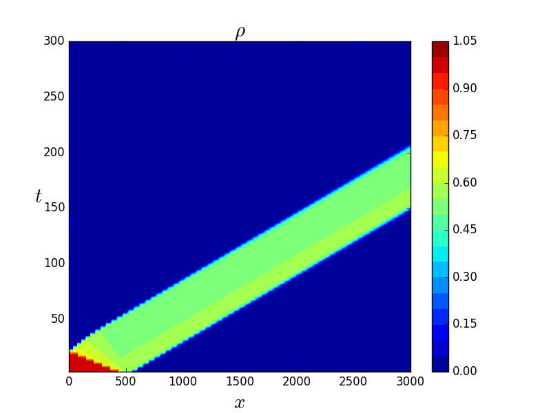 Figure 1
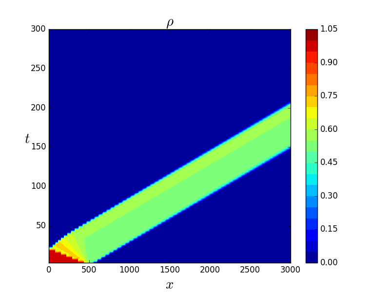 Figure 2
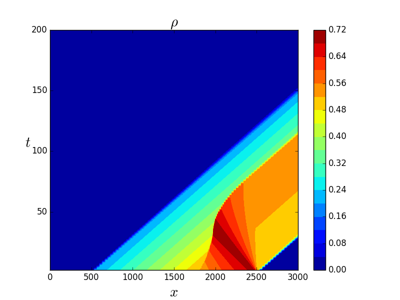 Figure 3
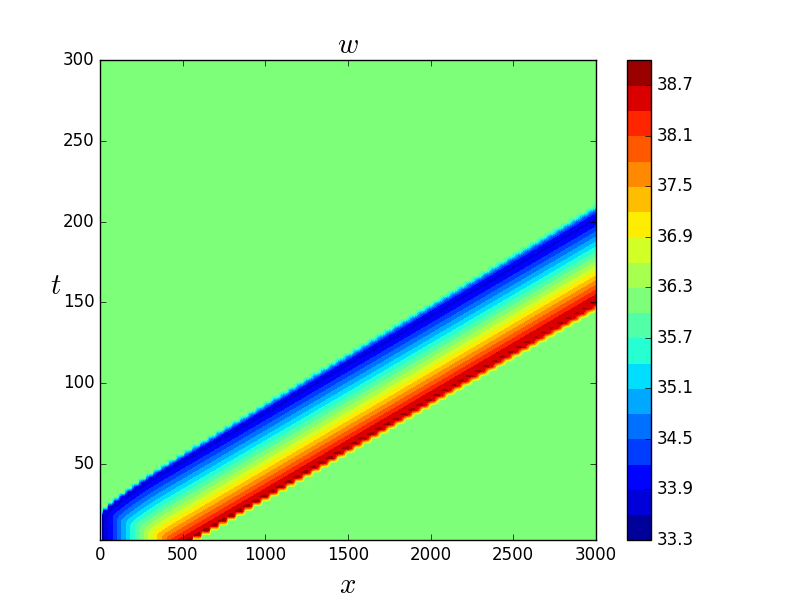 Figure 4
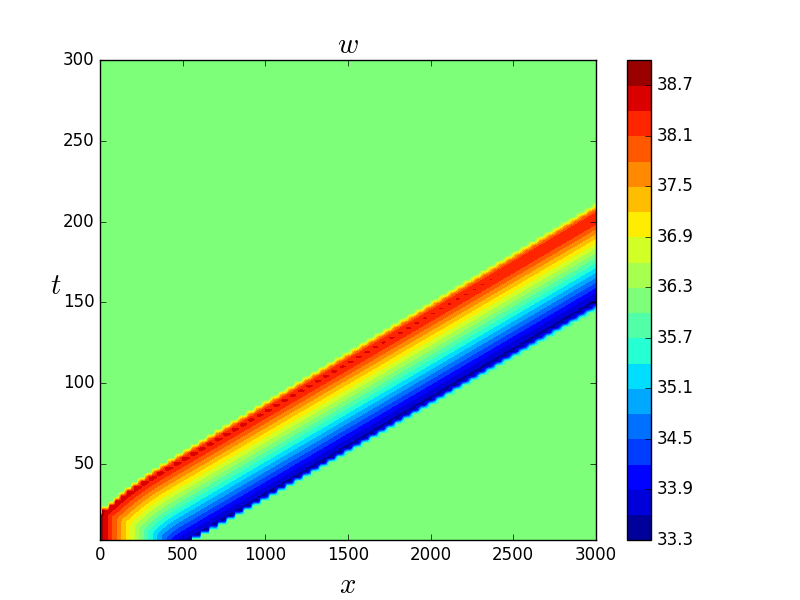 Figure 5
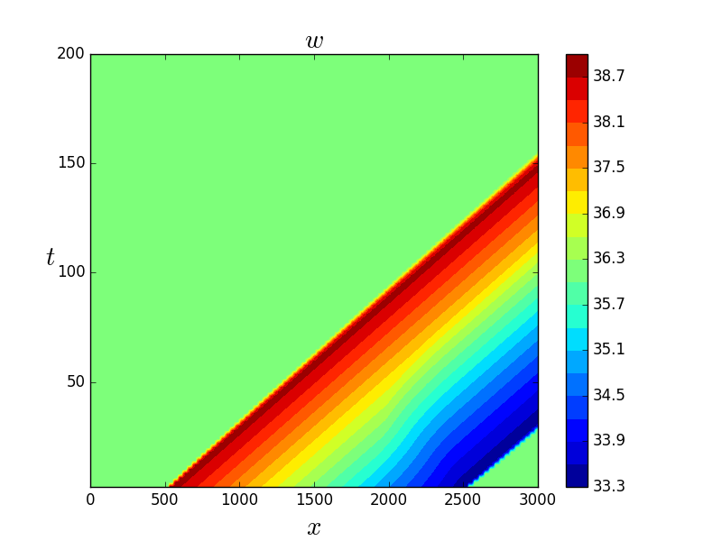 Figure 6
 Figure 7
 Figure 8
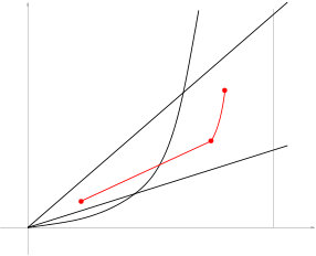 Figure 9
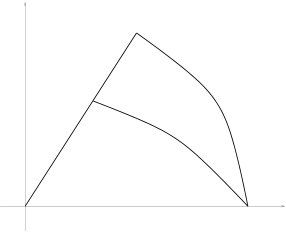 Figure 10
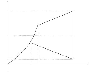 Figure 11
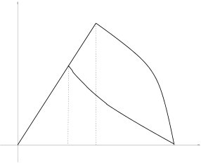 Figure 12
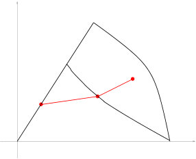 Figure 13
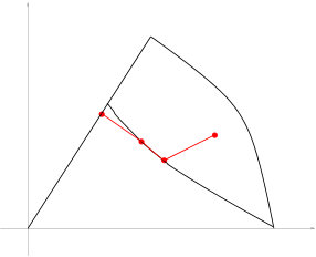 Figure 14
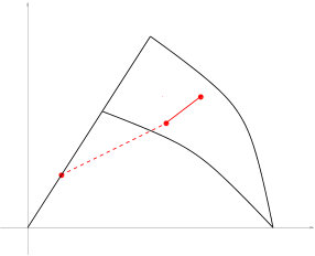 Figure 15
Peer Reviews
No public reviews on file for this paper yet. If you reviewed it on a platform where reviews are public (OpenReview, ICLR, NeurIPS, ICML), you can paste yours below so the community can read it here.
Videos
No videos yet. Explain this paper in a talk, walkthrough, or lecture? Add one.
The Godunov Method for a –Phase Model
M. Garavello Dipartimento di Matematica e Applicazioni, Università di Milano Bicocca, Via R. Cozzi 55, 20125 Milano, Italy. E-mail: [email protected]
F. Marcellini Dipartimento di Matematica e Applicazioni, Università di Milano Bicocca, Via R. Cozzi 55, 20125 Milano, Italy. E-mail: [email protected]
Abstract
We consider the Godunov numerical method to the phase-transition traffic model, proposed in [6], by Colombo, Marcellini, and Rascle. Numerical tests are shown to prove the validity of the method. Moreover we highlight the differences between such model and the one proposed in [1], by Blandin, Work, Goatin, Piccoli, and Bayen.
2000 Mathematics Subject Classification: 35L65, 90B20
Key words and phrases: –Phase Model, Continuum Traffic Models, Godunov Scheme, Hyperbolic Systems of Conservation Laws.
1 Introduction
Aim of this paper is to present the Godunov method for approximating the solutions to the –phase traffic model, introduced in [6] by Colombo, Marcellini, and Rascle. The model consists on the system of conservation laws
[TABLE]
where is the car density at time and at position , is a generalized momentum, is the avarage speed of cars, is a positive constant describing the maximum speed of cars, and is a given decreasing function. This model is an extension of the famous Lighthill-Whitham-Richards (LWR) model, see [15, 17], and it is obtained by assuming that different kinds of drivers have different maximal speeds , where , for suitable constants .
The model described by (1.1) belongs to the class of hyperbolic phase transition models for traffic, whose aim is to describe the different traffic regimes; see [11]. The pioneer work in this class is the model proposed in 2002 by Colombo; see [3, 4, 5]. Its distinctive feature is that the two phases are disconnected. Subsequently other phase transition models have been introduced in the literature; see [1, 6, 9, 12, 16]. In particular, the models in [1, 6], although very similar in the fundamental diagram, are indeed different, since solutions to Riemann problems have different structures and contain a different number of waves. Also the derivation of the two models is completely different: the construction in [1] is done imposing a priori two phases, the free and the congested one, while in [6] the two phases are obtained as a consequence of the speed limit .
In the present paper, we describe the Godunov numerical scheme for system (1.1). The Godunov method is a finite volume method for conservation laws; it is based on the solution to the Riemann problem in order to approximate the flux between two contiguous cells; see [10, 14]. In our setting, the fundamental diagram in the conserved variable is convex; hence the application of this method is straightforward. Instead the nonconvexity of the fundamental diagram for the model in [1] is a source of various problems for the Godunov method; see [2, 18].
The paper is organized as follow. In Section 2 we describe the 2-Phase Traffic Model (1.1). In Section 3 we make a comparison between the –Phase model (1.1) and that in [1]. Finally in Section 4, we describe the Godunov method to the model (1.1). Some numerical integrations conclude the paper.
2 Notations and Description of the Phase Transition Model
In this section we fix notations and we recall some properties concerning the –Phase traffic model introduced in [6]. As already said, the model (1.1) is an extension of the classical LWR model, given by the following scalar conservation law
[TABLE]
where is the traffic density and is the speed.
We consider the folllowing two assumptions on the speed:
- •
We assume that, at a given density, different drivers may choose different velocities, that is, we assume that , where is a function and is the maximal speed of a driver, located at position at time .
- •
We impose an overall bound on the speed .
We get the following system
[TABLE]
and then the model in (1.1), with the change of variables .
As a consequence of the introduction of the speed bound , system (1.1) produces two phases, the free and the congested one, described by the sets
[TABLE]
In Figure 1 it is represented the fundalmental digram in the coordinates and . Note that and are closed sets and . Note also that is one-dimensional in the plane of the fundamental diagram, while it is two-dimensional in the coordinates.
We recall the following assumptions:
(H-1)
are positive constants, with .
(H-2)
is such that
[TABLE]
(H-3)
Waves of the first family in the congested phase have negative speed.
We recall the eigenvalues, right eigenvectors, and Lax curves in :
[TABLE]
When , the 2-Lax curve through is the segment , .
In order to apply th Godunov’s method in Section 4, we recall the description of the solutions of the Riemann problem for the model (1.1). First, we recall all the possible waves in the solution.
- •
A Linear wave is a wave connecting two states in the free phase.
- •
A Phase Transition Wave is a wave connecting a left state with a right state satisfying .
- •
A Wave of the First Family is a wave connecting a left state with a right state such that .
- •
A Wave of the Second Family is a wave connecting a left state with a right state such that .
2.1 The Riemann Problem
Under the assumptions (H-1), (H-2) and (H-3), for all states , , the Riemann problem consisting of (1.1) with initial data
[TABLE]
admits a unique self similar weak solution constructed as follows:
- (1)
If , then the solution consists of a linear wave separating from . 2. (2)
If , then the solution consists of a wave of the first family (shock or rarefaction) between and a middle state , followed by a wave of the second family between and . 3. (3)
If and , then the solution consists of a wave of the first family separating from a middle state (which belongs to the intersection between and ) and by a linear wave separating from . 4. (4)
If and , then the solution consists of a phase transition wave between and a middle state (which is in ), followed by a wave of the second family between and .
3 Comparison with the Model in [1]
In this section we briefly describe the –Phase traffic model, introduced by Blandin, Work, Goatin, Piccoli and Bayen in [1], and we show the main differences with (1.1).
The phase transition traffic model in [1] has been developed as an extension of the Colombo phase transition model [3] and can be described by the following system
[TABLE]
where and , represent respectively the car traffic density and the linearized momentum, is the average speed of cars, while the sets and , respectively the free and the congested phases, are given by
[TABLE]
In (3.2), denotes the maximal density, is the maximal velocity attained by the vehicles in the free phase, and are respectively the minimum and the maximum value of the momentum , and the constants and are suitable constants in . The velocity is defined by
[TABLE]
where the equilibrium velocity represents the desired speed of cars when the density is . In the congested phase , when , the velocity of cars is the equilibrium velocity .
The models (1.1) and (3.1) have some similarities. Both models are described by two intersecting phases: the free phase and the two-dimensional congested phase. In Figures 1 and 2 the fundamental diagrams, respectively for (1.1) and for (3.1), are drawn. Note however that the free phase in (3.1) is one-dimensional both in the conserved quantity coordinates and in the coordinates . In the model (1.1) the free phase is two-dimensional in the conserved quantity coordinates .
The main difference between (1.1) and (3.1) lies in the solution of the Riemann problem, in particular when the left state belongs to the free phase and the right state to the congested one.
The following result for (1.1) holds.
Proposition 3.1
Consider the system (1.1) and fix the states , . The Riemann problem for (1.1) with the initial condition
[TABLE]
is solved with at most two waves.
Proof. Since and , the solution to the Riemann problem consists of a shock wave connecting to a middle state , possibly followed by a wave of the second family connecting to ; see Subsection 2.1 and Figure 3. This concludes the proof.
The following result for (3.1) holds.
Proposition 3.2
Consider the system (3.1) and fix the states , . The Riemann problem for (3.1) with the initial condition
[TABLE]
is solved with at most three waves.
Proof. We use here the notations in [1]. First define the intermediate state as he solution to the system
[TABLE]
Let be the speed of the phase transition wave connecting to . Its value is given by the Rankine-Hugoniot condition
[TABLE]
Denoting with the first eigenvalue of the Jacobian matrix of the flux at , the following possibilities hold.
. In this case, the solution to the Riemann problem consists of a phase transition wave connecting to , possibly followed by a contact discontinuity wave connecting to ; see Figure 3. 2. 2.
. Define the solution to
[TABLE]
The solution to the Riemann problem consists of a phase transition wave connecting to , of a rarefaction wave of the first family connecting to , and of contact discontinuity wave connecting to ; see Figure 3.
The proof is so concluded.
4 The Godunov Method
In this section we describe the Godunov method for the model (1.1) under the assumptions (H-1), (H-2), and (H-3); see [10, 13, 14]. We recall that such numerical scheme is a finite volume method, based on Riemann problems within computational cells in order to obtain the numerical fluxes.
Consider the system (1.1), with the conserved variables ; see Figure 1. Introduce the space discretization and the time dicretization satisfying the Courant-Friedrichs-Lewy conditions (see [7, 8]) as in [13]. Define , and, for all and all , the points , , the time , and the cell of length .
The Godunov method consists in the following steps.
Approximate an initial condition by a function , constant in each cell . Define for every . 2. 2.
Construct, for every and , the values by the recurrence formula
[TABLE]
where is a numerical flux at the interface , obtained through the solution of corresponding Riemann problems.
If , the numerical flux depends on the values and . Namely, denoting for simplicity with and respectively and , we have
[TABLE]
and
[TABLE]
Above is the middle state in the solution to the Riemann problem (2.4); see Subsection 2.1. Moreover the point is the middle point in the solution to the Riemann problem (2.4) when and ; see point (3) of Subsection 2.1. Note that the condition respectively greater or less than means that, by the Rankine-Hugoniot condition, the phase transition wave connecting and has strictly negative or positive speed.
4.1 Example: the case of a traffic light with increasing
We present here a simple situation of a road with a traffic light, which turns green at the initial time . At the beginning all the vehicles are stopped at the maximal density and is linearly increasing between and . We assume that the road is Km long, modeled by the real interval and the traffic light is located at position .
We choose, for the model (1.1), the parameters
[TABLE]
with and initial conditions
[TABLE]
In Figure 5 we show the contour plot for the numerical solution, obtained with the Godunov scheme, using the following numerical parameters:
[TABLE]
4.2 Example: the case of a traffic light with decreasing
We consider here a situation very similar to that of Subsection 4.1. The only difference is that the initial is decreasing between and . As before, we assume that the road is Km long, modeled by the real interval and the traffic light is located at position .
We choose, for the model (1.1), the parameters (4.4), the function , initial conditions
[TABLE]
In Figure 6 we show the contour plot for the numerical solution, obtained with the Godunov scheme, using the numerical parameters (4.6).
4.3 Example: increasing and decreasing
In this part we consider an example where the initial conditions are monotone functions: the density is increasing, while the maximal speed is decreasing. We assume that the road is Km long, modeled by the real interval .
We choose the parameters (4.4), the function , and the initial conditions
[TABLE]
In Figure 7 we show the contour plot for the numerical solution, obtained with the Godunov scheme, using the following numerical parameters:
[TABLE]
Acknowledgments
The authors were partial supported by the INdAM-GNAMPA 2016 project “Balance Laws: Theory and Applications”.
The reference list from the paper itself. Each links out to its DOI / PubMed record.
- 1[1] S. Blandin, D. Work, P. Goatin, B. Piccoli, and A. Bayen. A general phase transition model for vehicular traffic. SIAM J. Appl. Math. , 71(1):107–127, 2011.
- 2[2] C. Chalons and P. Goatin. Godunov scheme and sampling technique for computing phase transitions in traffic flow modeling. Interfaces Free Bound. , 10(2):197–221, 2008.
- 3[3] R. M. Colombo. Hyperbolic phase transitions in traffic flow. SIAM J. Appl. Math. , 63(2):708–721, 2002.
- 4[4] R. M. Colombo. Phase transitions in hyperbolic conservation laws. In Progress in analysis, Vol. I, II (Berlin, 2001) , pages 1279–1287. World Sci. Publ., River Edge, NJ, 2003.
- 5[5] R. M. Colombo, P. Goatin, and F. S. Priuli. Global well posedness of traffic flow models with phase transitions. Nonlinear Anal. , 66(11):2413–2426, 2007.
- 6[6] R. M. Colombo, F. Marcellini, and M. Rascle. A 2-phase traffic model based on a speed bound. SIAM J. Appl. Math. , 70(7):2652–2666, 2010.
- 7[7] R. Courant, K. Friedrichs, and H. Lewy. Über die partiellen Differenzengleichungen der mathematischen Physik. Math. Ann. , 100(1):32–74, 1928.
- 8[8] R. Courant, K. Friedrichs, and H. Lewy. On the partial difference equations of mathematical physics. IBM J. Res. Develop. , 11:215–234, 1967.