Short-time near-the-money skew in rough fractional volatility models
Christian Bayer, Peter K. Friz, Archil Gulisashvili, Blanka Horvath,, Benjamin Stemper

TL;DR
This paper advances the understanding of short-time near-the-money skew in rough fractional volatility models by deriving higher order moderate deviation estimates, extending the applicability of skew approximation formulas in option pricing.
Contribution
It sharpens large deviation results for rough volatility models, enabling analysis in a broader moderate deviations regime around the money.
Findings
Extended the range of at-the-money skew approximation formulas
Derived higher order moderate deviation estimates for rough volatility models
Enhanced analytical tractability in the near-the-money regime
Abstract
We consider rough stochastic volatility models where the driving noise of volatility has fractional scaling, in the "rough" regime of Hurst parameter . This regime recently attracted a lot of attention both from the statistical and option pricing point of view. With focus on the latter, we sharpen the large deviation results of Forde-Zhang (2017) in a way that allows us to zoom-in around the money while maintaining full analytical tractability. More precisely, this amounts to proving higher order moderate deviation estimates, only recently introduced in the option pricing context. This in turn allows us to push the applicability range of known at-the-money skew approximation formulae from CLT type log-moneyness deviations of order (recent works of Al\`{o}s, Le\'{o}n & Vives and Fukasawa) to the wider moderate deviations regime.
Click any figure to enlarge with its caption.
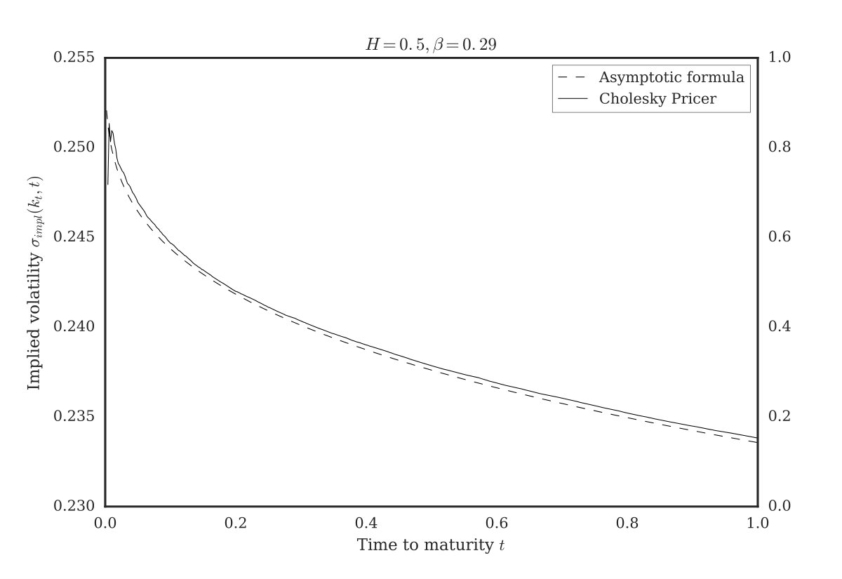 Figure 1
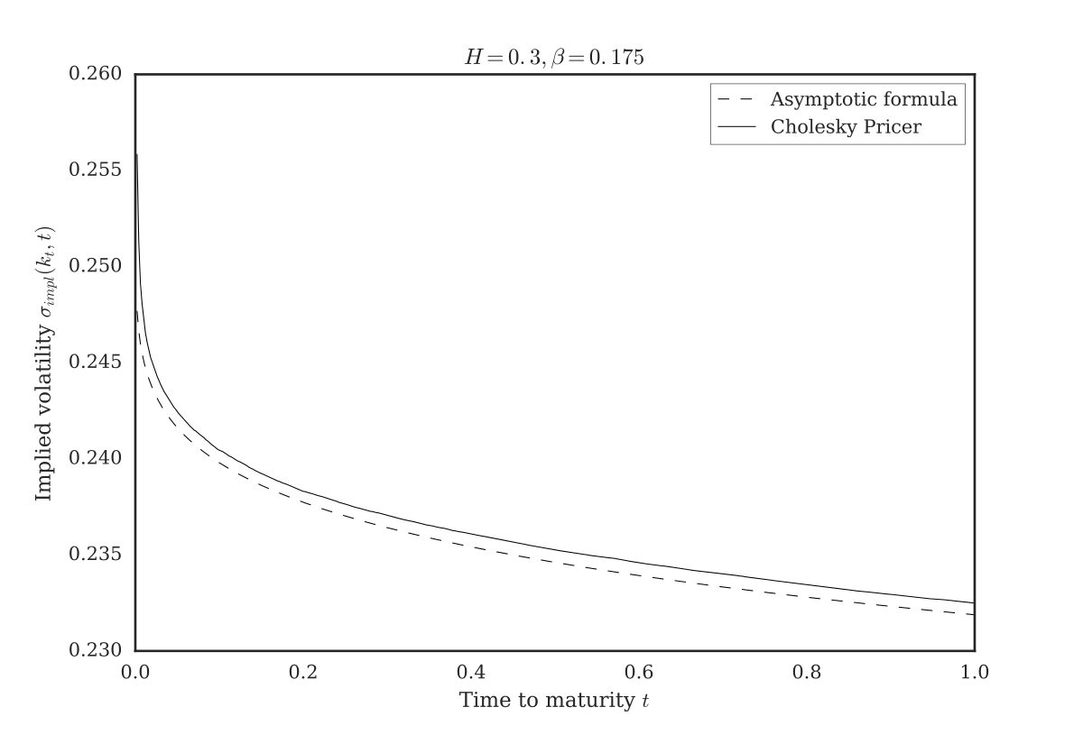 Figure 2
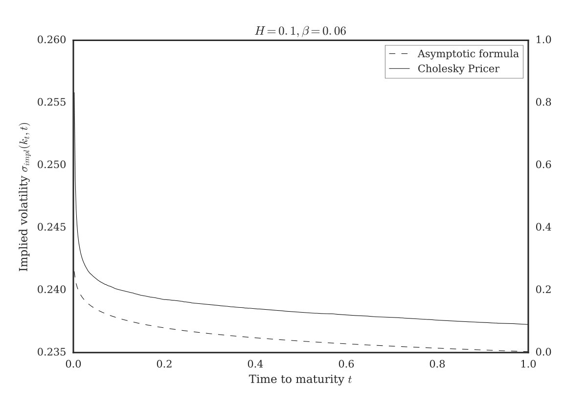 Figure 3
Peer Reviews
No public reviews on file for this paper yet. If you reviewed it on a platform where reviews are public (OpenReview, ICLR, NeurIPS, ICML), you can paste yours below so the community can read it here.
Videos
No videos yet. Explain this paper in a talk, walkthrough, or lecture? Add one.
Short-time near-the-money skew in rough fractional volatility models
C. Bayer, P. K. Friz, A. Gulisashvili, B. Horvath, B. Stemper
WIAS Berlin, TU and WIAS Berlin, Ohio University, Imperial College London, TU and WIAS Berlin
[email protected], [email protected], [email protected], [email protected], [email protected]
Abstract.
We consider rough stochastic volatility models where the driving noise of volatility has fractional scaling, in the ”rough” regime of Hurst parameter . This regime recently attracted a lot of attention both from the statistical and option pricing point of view. With focus on the latter, we sharpen the large deviation results of Forde-Zhang (2017) in a way that allows us to zoom-in around the money while maintaining full analytical tractability. More precisely, this amounts to proving higher order moderate deviation estimates, only recently introduced in the option pricing context. This in turn allows us to push the applicability range of known at-the-money skew approximation formulae from CLT type log-moneyness deviations of order (recent works of Alòs, León & Vives and Fukasawa) to the wider moderate deviations regime.
Key words and phrases:
rough stochastic volatility model, European option pricing, small-time asymptotics, moderate deviations
2010 Mathematics Subject Classification:
91G20, 60H30, 60F10, 60H07, 60G22, 60G18
We gratefully acknowledge financial support through DFG research grants FR2943/2 and BA5484/1 (C. Bayer, P.K. Friz, B. Stemper), European Research Council Grant CoG-683166 (P.K. Friz), and SNF Early Postdoc Mobility Grant 165248 (B. Horvath) respectively.
Contents
1. Introduction
Since the groundbreaking work of Gatheral, Jaisson and Rosenbaum [GJR14a], the past two years have brought about a gradual shift in volatility modeling, leading away from classical diffusive stochastic volatility models towards so-called rough volatility models. The term was coined in [GJR14a] and [BFG16], and it essentially describes a family of (continuous-path) stochastic volatility models where the driving noise of the volatility process has Hölder regularity lower than Brownian motion, typically achieved by modeling the fundamental noise innovations of the volatility process as a fractional Brownian motion with Hurst exponent (and hence Hölder regularity) . Here, we would also like to mention pioneering work on asymptotics for rough volatility models in [ALV07] and [Fuk11]. A major appeal of such rough volatility models lies in the fact that they effectively capture several stylized facts of financial markets both from a statistical [GJR14a, BLP16] and an option-pricing point of view [BFG16]. In particular, with regards to the latter point of view, a widely observed empirical phenomenon in equity markets is the “steepness of the smile on the short end” describing the fact that as time to maturity becomes small the empirical implied volatility skew follows a power law with negative exponent, and thus becomes arbitrarily large near zero. While standard stochastic volatility models with continuous paths struggle to capture this phenomenon, predicting instead a constant at-the-money implied volatility behaviour on the short end [Gat11], models in the fractional stochastic volatility family (and more specifically so-called rough volatility models) constitute a class, well-tailored to fit empirical implied volatilities for short dated options.
Typically, the popularity of asset pricing models hinges on the availability of efficient numerical pricing methods. In the case of diffusions, these include Monte Carlo estimators, PDE discretization schemes, asymptotic expansions and transform methods. With fractional Brownian motion being the prime example of a process beyond the semimartingale framework, most currently prevalent option pricing methods – particularly the ones assuming semimartingality or Markovianity – may not easily carry over to the rough setting. In fact, the memory property (aka non-Markovianity) of fractional Brownian motion rules out PDE methods, heat kernel methods and all related methods involving a Feynman-Kac-type Ansatz. Previous work has thus focused on finding efficient Monte Carlo simulation schemes [BFG16, BLP17, BFG*+*17] or – in the special case of the Rough Heston model – on an explicit formula for the characteristic function of the log-price (see [ER16]), thus in this particular model making pricing amenable to Fourier based methods. In our work, we rely on small-maturity approximations of option prices. This is a well-studied topic. See, e.g., [ALV07, GVZ15] (the at-the-money (ATM) regime) or [DFJV14a, DFJV14b, GJR14b, GHJ16, GVZ15] (the out-of-the-money (OTM) regime, where large deviations results are used). We also refer the reader to the papers [Fuk11, Fuk17, FZ17] concerning large deviations, and to [MT16, Osa07, MS03, MS07] for related work. Based on the moderate deviations regime, Friz et al. [FGP17] have recently introduced another regime called moderately-out-of-the-money (MOTM), which, in a sense, effectively navigates between the two regimes mentioned above, by rescaling the strike with respect to the time to maturity. This approach has various advantages. On the one hand, it reflects the market reality that as time to maturity approaches zero, strikes with acceptable bid-ask spreads tend to move closer to the money (see [FGP17] for more details). On the other hand, it allows us to zoom in on the term structure of implied volatility around the money at a high resolution scale. To be more specific, our paper adds to the existing literature in two ways. First, we obtain a generalization of the Osajima energy expansion [Osa15] to a non-Markovian case, and using the new expansion, we extend the analysis of [FGP17] to the case, where the volatility is driven by a rough fractional Brownian motion. Indeed, Laplace approximation methods on Wiener space in the spirit of Ben Arous [BA88] and Bismut [Bis84] remain valid in the present context, and our analysis builds upon this framework in a fractional setting. Second, we use an asymptotic expansion going back to Azencott [Aze85] to bypass the need for deriving an asymptotic expansion of the density of the underlying process to obtain asymptotics for option prices. We display the potential prowess of this approach by applying it to our specific model, and derive asymptotics for call prices directly, irrespectively of corresponding density asymptotics. Finally, using a version of the ”rough Bergomi model” [BFG16], we demonstrate numerically that our implied volatility asymptotics capture very well the geometry of the term structure of implied volatility over a wide array of maturities, extending up to a year.
The paper is organized as follows: In Section 2 we set the scene, describing the class of models included in our framework ((2.1) and (2.2)) and recalling some known results ((2.4) and (2.7)), which are the starting point of our analysis. Most importantly, we argue that for small-time considerations it would suffice to restrict our attention to a class of stochastic volatility models of the form (2.3) with a volatility process driven by a Gaussian Volterra process such as in (2.2). We formulate general assumptions on the Volterra kernel (Assumptions 2.1 and 2.5) and on the function in (2.3) (Assumption 2.4) under which our results are valid. In Section 3 we gather our main results, concerning a higher order expansion of the energy (Theorem 3.1), and a general expansion formula for the corresponding call prices. We derive the classical Black-Scholes expansion for the call price, using the latter result mentioned above. In addition, in Section 3 we formulate moderate deviation expansions, which allow us to derive the corresponding asymptotic formulae for implied volatilities and implied volatility skews. Finally, Section 4 displays our simulation results. Sections 5, 6 and 7 are devoted to proofs of the energy expansion, the price expansion and the moderate deviations expansion, respectively. In the appendix, we have collected some auxiliary lemmas, which are used in different sections.
2. Exposition and assumptions
We consider a rough stochastic volatility model, normalized to and , of the form suggested by Forde-Zhang [FZ17]
[TABLE]
Here are two independent standard Brownian motions, a correlation parameter, and . Then is another standard Brownian motion which has constant correlation with the factor , which drives the stochastic volatility
[TABLE]
Here is some real-valued function, typically smooth but not bounded, and we will denote by the spot volatility, with a Gaussian (Volterra) process of the form
[TABLE]
for some kernel , which shall be further specified in Assumptions 2.1 and 2.5 below. The log-price satisfies
[TABLE]
Recall that by Brownian scaling, for fixed ,
[TABLE]
As a direct consequence, classical short-time SDE problems can be analyzed as small-noise problems on a unit time horizon. For our analysis, it will also be crucial to impose such a scaling property on the Gaussian process (more precisely, on the kernel in (2.2)) driving the volatility process in our model:
Assumption 2.1** (Small time self-similarity).**
There exists a number with and a function , , such that
[TABLE]
In fact, we will always have
[TABLE]
which covers the examples of interest, in particular standard fractional Brownian motion or Riemann-Liouville fBM with explicit kernel . (This is very natural, even from a general perspective of self-similar processes, see [Lam62].)
We insist that no (global) self-similarity of is required, as only for arbitrarily small matters.
Remark 2.2*.*
It should be possible to replace the fractional Brownian motion by a certain fractional Ornstein-Uhlenbeck process in the results obtained in this paper. Intuitively, this replacement creates a negligible perturbation (for ) of the fBm environment. A similar situation was in fact encountered in [CF10], where fractional scaling at times near zero was important. To quantify the perturbation, the authors of [CF10] introduced an easy to verify coupling condition (see Corollary 2 in [CF10]). It should be possible to employ a version of this condition in the present paper to justify the replacement mentioned above. We will however not pursue this point further here.
Remark 2.3*.*
Throughout this article, one can consider a classical (Markovian, diffusion) stochastic volatility setting by taking , or equivalently , by simply ignoring all hats ( ) in the sequel. In particular then, in all subsequent formulae.
General facts on large deviations of Gaussian measures on Banach spaces [DS89] such as the path space imply that a large deviation principle holds for the triple , with speed and rate function
[TABLE]
where
[TABLE]
for , the space of absolutely continuous paths with derivative
[TABLE]
This enables us to derive a large deviations principle for in (2.3): the (local) small-time self-similarity property of (Assumption 2.1) implies that where
[TABLE]
For what follows, it will be convenient to consider a rescaled version of (2.3)
[TABLE]
Under a linear growth condition on the function , Forde–Zhang [FZ17] use the extended contraction principle to establish a large deviations principle for () with speed . More precisely, with
[TABLE]
the rate function is given by
[TABLE]
where denotes the inner product on . Several other proofs (under varying assumptions on ) have appeared since [JPS17, BFG*+*17, Gul17].
As a matter of fact, this paper relies on moderate - rather than large - deviations, as emphasized in (iiic) below. To this end, let us make
Assumption 2.4**.**
- (i)
(Positive spot vol) Assume is smooth with . 2. (ii)
(Roughness) The Hurst parameter satisfies . 3. (iiia)
(Martingality) The price process is a martingale. 4. (iiib)
(Short-time moments) : .
While condition (iiia) hardly needs justification, we emphasize that conditions (iiia-b) are only used to the extent that they imply condition (iiic) given below (which thus may replace (iiia-b) as an alternative, if more technical, assumption). The reason we point this out explicitly is that all the conditions (iiia-c) are implicit (growth) conditions on the function . For instance, (iiia-b) was seen to hold under a linear growth assumption [FZ17], whereas the log-normal volatility case (think of ) is complicated. Martingality, for instance, requires and there is a critical moment , even when . See [Sin98, Jou04, LM07] for the case and the forthcoming work [FG18] for the general rough case . We view (iiic) simply as a more flexible condition that can hold in situations where (iiib) fails.
- (iiic)
(Call price upper moderate deviation bound) For every , and every fixed , and ,
[TABLE]
This condition is reminiscent of the “upper part” of the large deviation estimate obtained in [FZ17]
[TABLE]
If fact, if one formally applies this with replaced by , followed by Taylor expanding the rate function,
[TABLE]
one readily arrives at the estimate (iiic). Unfortunately, in (2.8), which is a serious obstacle in making this argument rigorous. Instead, we will give a direct argument (Lemma 7.1) to see how (iiia-b) implies (iiic).
In the sequel, we will use another mild assumption on the kernel.
Assumption 2.5**.**
The kernel has the following properties
- (i)
has a continuous (in ) version on .
- (ii)
.
Note that the Riemann-Liouville kernel , satisfies Assumption 2.5.
Remark 2.6*.*
Assumption 2.5 implies that the Cameron-Martin space of is given by the image of under , i.e.,
[TABLE]
See Lemma 5.3 and Remark 5.4 for more details. A reference and also a sufficient condition for Assumption 2.5 (i) can be found e.g. in [Dec05, Section 3].
3. Main results
The following result can be seen as a non-Markovian extension of work by Osajima [Osa15]. The statement here is a combination of Theorem 5.10 and Proposition (5.14) below. Recall that represents spot-volatility. We also set .
Theorem 3.1** (Energy expansion).**
The rate function (or energy) in (2.7) is smooth in a neighbourhood of (at-the-money) and it is of the form
[TABLE]
The next result is an exact representation of call prices, valid in a non-Markovian generality, and amenable to moderate- and large-deviation analysis (Theorem 3.4 below) as well as to full asymptotic expansions, which will be explored in forthcoming work.
Theorem 3.2** (Pricing formula).**
For a fixed log-strike and time to maturity , set , where and , as before. Then we have
[TABLE]
where
[TABLE]
and is a random variable of the form
[TABLE]
with a centred Gaussian random variable, explicitly given in equation (6.3) below, and is a (random) remainder term, in the sense of a stochastic Taylor expansion in , see Lemma 6.2 for more details.
Example 3.3** (Black-Scholes model).**
We fix volatility , and so that and all can be omitted. Energy is given by and
[TABLE]
with independent of . Moreover,
[TABLE]
with , and, in terms of the standard Gaussian cdf ,
[TABLE]
Using the expansion , as one deduces, for fixed , the asymptotic relation, as ,
[TABLE]
We will be interested (cf. Theorem 3.4) in replacing by for . This gives and the above analysis, now based on , remains valid111More terms in the expansion of are needed. for in the “moderate” regime and we obtain
[TABLE]
Let us point out, for the sake of completeness, that a similar expansion is not valid for . To see this, first note that (3.1) implies that is precisely the ATM call price with time from expiration. Well-known ATM asymptotics then imply that as . These asymptotics are unchanged in case of out-of-moneyness (“almost-at-the-money” in the terminology of [FGP17]), which readily implies
[TABLE]
At last, we have the borderline case , or . From e.g. [MKN11, Thm 3.1], we see that with positive constant . A look at (3.1) then reveals
[TABLE]
For the call price expansion in the large / moderate deviations regime, , the polynomial in -behaviour of (3.5) implies that the -term in the pricing formula will be negligible on the moderate / large deviation scale, in the sense for any , we have as . Consequently, with , for , , , we get the “moderate” Black-Scholes call price expansion,
[TABLE]
While the above can be confirmed by elementary analysis of the Black–Scholes formula, the following theorem exhibits it as an instance of a general principle. See [FGP17] for a general diffusion statement.
Theorem 3.4** (Moderate Deviations).**
In the rough volatility regime , consider log-strikes of the form
[TABLE]
(i) For , and every , we have
[TABLE]
(ii) For , and every , we have
[TABLE]
Moreover,
[TABLE]
where is the inner product in .
Remark 3.5*.*
In principle, further terms (of order ) can be added to this expansion of log call prices, given that the energy has sufficient regularity, see Theorem 3.6. We also note that, for small enough , the error term can be omitted. In any case, one can replace the additive error bounds by (cruder) ones, where the right-most term in the expansion is multiplied with , as was done in [FGP17].
Proof of Theorem 3.4.
We apply Theorem 3.2 with , i.e., with . In particular, we so get, with and ,
[TABLE]
The technical Proposition 7.3 asserts that, for fixed , the factor is negligible in the sense that, for every ,
[TABLE]
The theorem now follows immediately from the Taylor expansion of around (see Theorem 3.1), plugging in . Indeed, replacing by the Taylor-jet seen in (i),(ii), leads exactly to an error term , resp. . ∎
Fix real numbers , , , and an integer . For every , set
[TABLE]
and denote
[TABLE]
Here, can be arbitrarily small. It is clear that for all small and small enough,
[TABLE]
while
[TABLE]
The following statement provides an asymptotic formula for the implied variance.
Theorem 3.6**.**
Suppose and small enough. Then as ,
[TABLE]
The -estimate in (3.6) depends on , , , , and . It is uniform on compact subsets of with respect to the variable .
Remark 3.7*.*
Using the multinomial formula, we can represent the expression on the left-hand side of (3.6) in terms of certain powers of . However, the coefficients become rather complicated.
Remark 3.8*.*
Let an integer be fixed, and suppose we would like to use only the derivatives for in formula (3.6) to approximate . Then, the optimal range for is the following: . On the other hand, if is outside of the interval , more derivatives of the energy function at zero may be needed to get a good approximation of the implied variance in formula (3.6).
We will next derive from Theorem 3.6 several asymptotic formulas for the implied volatility. In the next corollary, we take .
Corollary 3.9**.**
As ,
[TABLE]
Corollary 3.9 follows from Theorem 3.6 with , the equality
[TABLE]
given in Theorem 3.4, and the Taylor expansion as .
In the next corollary, we consider the case where .
Corollary 3.10**.**
Suppose . Then, as ,
[TABLE]
Corollary 3.10 follows from Theorem 3.6 with , formula (3.8), the equality
[TABLE]
(see Theorem 3.4), and the expansion as .
Using Corollary 3.10, we establish the following implied volatility skew formula in the moderate deviation regime.
Corollary 3.11**.**
Let , , and fix with . Then as ,
[TABLE]
Remark 3.12*.*
Corollary 3.11 complements earlier works of Alòs et al. [ALV07] and Fukasawa [Fuk11, Fuk17]. For instance, the following formula can be found in [Fuk17, p. 6], see also [Fuk11, p. 14]:
[TABLE]
In formula (3.12), we employ the notation used in the present paper. Our analysis shows that the applicability range of skew approximation formulas is by no means restricted to the Central Limit Theorem type log-moneyness deviations of order . It also includes the moderate deviations regime of order . The previous rate is clearly as .
Remark 3.13* (Symmetry).*
Write for the “Itô-type map”
[TABLE]
It equals, in law, , and indeed all our formulae are invariant under this transformation. In particular, the skew remains unchanged when the pair is replaced by .
4. Simulation results
We verify our theoretical results numerically with a variant of the rough Bergomi model [BFG16] which fits nicely into the general rough volatility framework considered in this paper. As before, the model has been normalized such that and . We let be two independent Brownian motions and with such that is another Brownian motion having constant correlation with . For some spot volatility and volatility of volatility parameter , we then assume the following dynamics for some asset :
[TABLE]
where is a Riemann-Liouville fBM given by
[TABLE]
The approach taken for the Monte Carlo simulations of the quantities we are interested in is the one initially explored in the original rough Bergomi pricing paper [BFG16]. That is, exploiting their joint Gaussianity, where we use the well-known Cholesky method to simulate the joint paths of on some discretization grid . With (4.2) being an explicit function in terms of the rough driver, an Euler discretisation of the Ito SDE (4.1) on then yields estimates for the price paths.
The Cholesky algorithm critically hinges on the availability and explicit computability of the joint covariance matrix of whose terms we readily compute below.222 Note that expressions for the exact same scenario have have been computed before in the original pricing paper [BFG16], yet in that version the expression for the autocorrelation of the fBM was incorrect. We compute and state here all the relevant terms for the sake of completeness.
Lemma 4.1**.**
For convenience, define constants and and define an auxiliary function by
[TABLE]
*where denotes the Gaussian hypergeometric function [Olv10]. Then the joint process has zero mean and covariance structure governed by
\begin{cases}\operatorname{Var}[\widehat{B}_{t}^{2}]=t^{2H},&\text{for t\geq 0,}\\ \operatorname{Cov}[\widehat{B}_{s}\widehat{B}_{t}]=t^{2H}G\left(s/t\right),&\text{for s>t\geq 0,}\\ \operatorname{Cov}[\widehat{B}_{s}Z_{t}]=\rho D_{H}\left(s^{H+\frac{1}{2}}-\left(s-\min(t,s)\right)^{H+\frac{1}{2}}\right),&\text{for t,s\geq 0,}\\ \operatorname{Cov}[Z_{t}Z_{s}]=\min(t,s),&\text{for t,s\geq 0.}\end{cases}**
Numerical simulations333 The Python 3 code used to run the simulations can be found at github.com/RoughStochVol. confirm the theoretical results obtained in the last section. In particular - as can be seen in Figure LABEL:fig:pub_roughimpvol – the asymptotic formula for the implied volatility (3.9) captures very well the geometry of the term structure of implied volatility, with particularly good results for higher and worsening results as . Quite surprisingly, despite being an asymptotic formula, it seems to be fairly accurate over a wide array of maturities extending up to a single year.
5. Proof of the energy expansion
Consider
[TABLE]
where for a fixed Volterra kernel (recall (2.3) in the previous section). We study the small noise problem where is replaced by . The following proposition roughly says that
[TABLE]
Proposition 5.1** (Forde-Zhang [FZ17]).**
Under suitable assumptions (cf. Section 2), the rescaled process satisfies an LDP (with speed ) and rate function
[TABLE]
where
[TABLE]
The rest of this section is devoted to analysis of the function as defined in (5.1). First, we derive the first order optimality condition for the above minimization problem.
Proposition 5.2** (First order optimality condition).**
For any we have at any local minimizer of the functional in (5.1) that
[TABLE]
for all .
Proof.
We denote whenever for a small parameter . We expand
[TABLE]
If is a minimizer then has a minimum at for all . We expand
[TABLE]
As a consequence, we must have, for and every
[TABLE]
Recall , any . We now test with for a fixed and obtain
[TABLE]
5.1. Smoothness of the energy
Having formally identified the first order condition for minimality in (5.1), we will now show that the energy is a smooth function. More precisely, we will use the implicit function theorem to show that the minimizing configuration is a smooth function in (locally at ). As is a smooth function, too, this will imply smoothness of , at least in a neighborhood of [math].
As the Cameron-Martin space of the process continuously embeds into , maps continuously into , i.e., there is a constant such that for any we have
[TABLE]
This result will follow from
Lemma 5.3**.**
Let be a continuous, centred Gaussian process and its Cameron-Martin space. Then we have the continuous embedding . That is, for some constant ,
[TABLE]
Proof.
By a fundamental result of Fernique, applied to the law of as Gaussian measure on the Banach space , the random variable has Gaussian integrability. In particular,
[TABLE]
On the other hand, a generic element can be written as where is a centred Gaussian random variable with variance , see, e.g., [FH14, page 150]. By Cauchy–Schwarz,
[TABLE]
and conclude by taking the over on the l.h.s. over . ∎
Remark 5.4*.*
Assume is of Volterra form, i.e. . Then it can be shown (see [Dec05, Section 3]) that is the image of under the map
[TABLE]
and In particular then, applying the above with , gives
[TABLE]
5.1.1. The uncorrelated case
We start with the case as the formulas are much simpler in this case.
By Proposition 5.2, any local optimizer of the functional in the uncorrelated case satisfies for any
[TABLE]
We define a map by
[TABLE]
Hence, for given , any local optimizer must solve . As one particular solution is given by the pair , we are in the realm of the implicit function theorem. We need to prove that
- •
is locally smooth (in the sense of Fréchet);
- •
is invertible in .
Note that invertibility should hold for small enough, as for some , which is invertible as long as has a bounded norm for sufficiently small .
Remark 5.5*.*
The method of proof in this section is purely local in . Hence, we only really need smoothness of locally around [math]. Note, however, that stochastic Taylor expansions used in Section 6 will actually require global smoothness of .
Lemma 5.6**.**
The functions and defined by
[TABLE]
are smooth in the sense of Fréchet.
Proof.
For we note that the Gateaux derivative of satisfies
[TABLE]
By Lemma 5.3, we can bound
[TABLE]
for .444More precisely, since neither nor its derivatives need to be bounded, we need to actually work with a local version of the above estimate, for instance by replacing the max with a sup over a compact set containing . Thus, is a multi-linear form on with operator norm independent of . As is continuous, we conclude that as given above is, in fact, a Fréchet derivative.
Let us next consider the functional . Note that
[TABLE]
for . Hence, Assumption 2.5 implies that
[TABLE]
We see that the multi-linear map has operator norm bounded by
[TABLE]
independent of . From continuity of , it follows that is the ’th Fréchet derivative. ∎
Theorem 5.7** (Zero correlation).**
Assuming , the energy (as defined in (5.1)) is smooth in a neighborhood of .
Proof.
By construction, we have
[TABLE]
for defined by
[TABLE]
Here,
[TABLE]
As verified above, is smooth in the sense of Fréchet. Trivially, is invertible and . Therefore, the implicit function theorem implies that there are open neighborhoods and of and , respectively, and a smooth map from to such that and is unique in with this property.
For the energy, we prove that in a neighborhood of . First of all, we show that a minimizer exists. If not, there is a function with . For small enough such a must be inside a ball with radius around , as and . Then note that for any
[TABLE]
where denotes the second derivative of . By continuity, stays positive definite for in a neighborhood of . As noted, for small enough, both and (and the line connecting them) lie in this neighborhood. For , this implies
[TABLE]
since and . This contradicts the assumption that , and we conclude that is, indeed, a minimizer of , implying that locally.
Finally, as is smooth and is smooth, we see that is smooth in a neighborhood of [math]. (Note that this arguments relies on , implying that for in a neighborhood to [math].) ∎
Remark 5.8*.*
Classical counter-examples in the context of the direct method of calculus of variations show that the step of verifying the existence of a minimizer should not be taken too lightly. For instance, the functional
[TABLE]
does not have a minimizer in , but can be made arbitrarily close to [math] by choosing piecewise-linear functions with slope oscillating around [math]. We refer to any text book on calculus of variations. In the situation above, local “convexity” in the sense of a positive definite second derivative prevents this phenomenon. An alternative method of proof for the existence of a minimizer is to show that is (lower semi-) continuous in the weak sense.
5.1.2. The general case
In the general case (cf. Proposition 5.2), we define the function by
[TABLE]
where are defined by
[TABLE]
.
One easily checks that , , are smooth in the Fréchet sense.
Lemma 5.9**.**
The functions , and are smooth in Fréchet sense.
Proof.
The proof of smoothness is clear. We report the actual derivatives. For we get
[TABLE]
For and, respectively, , we obtain
[TABLE]
and
[TABLE]
Theorem 5.10**.**
Let be smooth with . Then the energy as defined in (5.1) is smooth in a neighborhood of .
Proof.
The proof is similar to the proof of Theorem 5.7. In fact, the only difference is in establishing invertibility of and the existence of a minimizer.
Note that (5.5) contains three terms. The derivative of the first term () is always equal to . For the second term, we note that
[TABLE]
Hence, the only non-vanishing contribution to the derivative of the second term evaluated in direction at , and is
[TABLE]
For the same reason, the derivative of the third term at vanishes entirely. Hence,
[TABLE]
It is easy to see that is invertible. Indeed, let us construct the pre-image of some . At we have
[TABLE]
implying . For , we then get
[TABLE]
or .
For existence of the minimizer, note that
[TABLE]
which is again positive definite. ∎
Remark 5.11*.*
Note that we do not really need infinite smoothness of if we only want partial smoothness of . Indeed, it is easy to show that implies that (locally at [math]).
5.2. Energy expansion
Having established smoothness of the energy as well as of the minimizing configuration locally around , we can proceed with computing the Taylor expansion of around . We will once more rely on the first order optimality condition given in Proposition 5.2. Plugging the Taylor expansion of into will then give us the local Taylor expansion of .
5.2.1. Expansion of the minimizing configuration
Theorem 5.12**.**
We have
[TABLE]
Remark 5.13* (Non-Markovian transversality).*
In the RL-fBM case, with one computes
[TABLE]
Interestingly, the transversality condition known from the Markovian setting (, which readily translates to there) remains valid here (for ), at least to order , in the sense that
[TABLE]
Proof of Theorem 5.12.
**First order expansion:
**Up to the order needed in order to get the first order term, we have
[TABLE]
Therefore,
[TABLE]
This yields for the first order term in (5.2)
[TABLE]
Setting , we get
[TABLE]
which is solved by . Inserting this term back into the equation for , we get
[TABLE]
Second order expansion:
Using (5.8) and the ansatz , we re-compute the relevant terms appearing in the (5.2). We have
[TABLE]
and analogously for replaced by , . This implies
[TABLE]
Using the notation introduced earlier, we have
[TABLE]
This directly implies
[TABLE]
We next compute some auxiliary terms appearing in (5.2).
[TABLE]
The corresponding denominator is . Using the formula
[TABLE]
we obtain
[TABLE]
For the second term in (5.2), let
[TABLE]
The corresponding denominator is . Hence,
[TABLE]
Combining (5.9) and (5.10), we get
[TABLE]
We shall next compute . Taking the second order terms on both sides and letting , we obtain
[TABLE]
Moving to the other side with and collecting terms on the right hand side, we arrive at
[TABLE]
We conclude that
[TABLE]
Hence, we obtain
[TABLE]
5.2.2. Energy expansion in the general case
Now we compute the Taylor expansion of as defined in Proposition 5.1. We start with the second term. Plugging in the optimal path (and using as ) we obtain
[TABLE]
Inserting into the above formula for , we get
[TABLE]
Recall the denominator
[TABLE]
Using the expansion of a fraction
[TABLE]
we obtain from
[TABLE]
We note that
[TABLE]
Adding both terms, we arrive at the
Proposition 5.14**.**
The energy expansion to third order gives
[TABLE]
5.2.3. Energy expansion for the Riemann-Liouville kernel
Let us specialize the energy expansion given in Proposition 5.14 for the Riemann-Liouville fBm. Choose and recall that the kernel takes the form . We get
[TABLE]
The key term appearing in the energy expansion now gives
[TABLE]
Plugging formula (5.2.3) into the energy expansion, we obtain the energy expansion for the Riemann-Liouville fractional Browian motion
[TABLE]
For completeness, let us also fully describe the time-dependence of the second order term in the expansion of the optimal trajectory . Unlike the first order time, here we do not have a linear movement any more. Indeed
[TABLE]
6. Proof of the pricing formula
Fix and where and . We have
[TABLE]
where we recall
[TABLE]
Consider a Cameron-Martin perturbation of . That is, for a Cameron-Martin path consider a measure change corresponding to a transformation (transforming the Brownian motions to Brownian motions with drift), we obtain the Girsanov density
[TABLE]
Under the new measure, becomes , where
[TABLE]
Definition 6.1**.**
For fixed , write if . Call such admissible for arrival at log-strike . Call the cheapest admissible control, which attains
[TABLE]
where we recall that and
[TABLE]
For any Cameron-Martin path , the perturbed random variable admits a stochastic Taylor expansion with respect to .
Lemma 6.2**.**
Fix and define accordingly. Then
[TABLE]
where is a Gaussian random variable, given explicitly by
[TABLE]
and
[TABLE]
Proof.
By a stochastic Taylor expansion for the controlled process with control as in Definition 6.1 and thanks to , we have at
[TABLE]
Collecting terms in powers of and with the random variable as in (6.3) (recalling that ), we have
[TABLE]
furthermore, since , by the definition of , it holds that
[TABLE]
This proves the statement (6.2) and the statement that is Gaussian is immediate from the form (6.3). ∎
Finally, we determine an explicit form of the Girsanov density for the choice where in (6.1) are chosen the cheapest admissible control (cf. Definition 6.1. Similarly to classical works of Azencott, Ben Arous and others, see, for instance, [BA88], we show that the stochastic integrals in the exponent of are proportional to the first order term (with factor ) when evaluated at the minimizing configuration .
Lemma 6.3**.**
We have
[TABLE]
Proof.
See Lemma A.2. ∎
With these preparations in place, we are now ready to prove the pricing formula from Section 3.
Proof of Theorem 3.2.
With a Girsanov factor (all integrals on )
[TABLE]
and (evaluated at the minimizer)
[TABLE]
we have, setting
[TABLE]
7. Proof of the moderate deviation expansions
In Section 2, we pointed out that (iiic) is exactly what one get from (call price) large deviations (2.8), if heuristically applied to . We now sketch a proper derivation based on moderate deviations.
Lemma 7.1**.**
Assume (iiia-b) from Assumption 2.4. Then an upper moderate deviation estimate holds both for calls and digital calls. That is, we have
- (iiic)
For every , and every fixed , and ,
[TABLE]
and also
[TABLE]
Proof.
(Sketch) Recall smooth but unbounded and recall . In case of and a large deviation principle (LDP) for is readily reduced, via exponential equivalence, to a LDP for the family of stochastic Itô integrals given by for some Brownian , -correlated with . There are then many ways to establish a LDP for this family. A particularly convenient one, that requires no growth restriction on , uses continuity of stochastic integration with respect to the rough path in suitable metrics, for which a LDP is known [FH14, Ch 9.3]. It was pointed out in [BFG*+*17] that a similar reasoning is possible when , the rough path is then replaced by a “richer enhancement” of , the precise size of which depends on , for which again one has a LDP. A moderate deviation priniple (MDP) for is a LDP for for . This can be reduced to a LDP, with , for
[TABLE]
with speed . Also, convergens (with all derivatives) locally uniformly to the constant function , and one checks that is exponentially equivalent to the (Gaussian) family given by , with law which gives (7.1), even with equality. (Showing this exponential equivalence can again be done for without growth restrictions.)
We have not yet used either assumption (iiia-b). These become important in order to extend estimate (7.1) to the case of genuine call payoffs. We can follow here a well-known argument (Forde-Jacquier, Pham, …) with the “moderate” caveat to carry along a factor . In fact, this is close in spirit to what already happens with rough volatility where one has to carry along a factor . The remaining details then follow essentially “Appendix C. Proof of Corollary 4.13., part (ii) upper bound” of [FZ17], noting perhaps that the authors use their assumptions to show validity of what we simply assumed as condition (iiib), and also that one works with the quadratic rate function throughout. ∎
Remark 7.2*.*
By an easy argument similar to “Appendix C. Proof of Corollary 4.13., part (i) lower bound” of [FZ17] one sees that validity of the call price upper bound (iiic) implies the corresponding digital call price upper bound (7.1.) For this reason, we only emphasized (iiic) but not (7.1) in Section 2.
In a classical work Azencott [Aze82] (see also [Aze85], [BA88, Théorème 2]) obtained asymptotic expansions of functionals of Laplace type on Wiener space, of the type “”, for small noise diffusions . This refines the large deviation (equivalently: Laplace) principle of Freidlin–Wentzell for small noise diffusions. In a nutshell, for fixed , Azencott gets expansions of the form . His ideas (used by virtually all subsequent works in this direction) are a Girsanov transform, to make the minimizing path “typical”, followed by localization around the minimizer (justified by a good large deviation principle), and finally a local (stochastic Taylor) type analysis near the minimizer. None of these ingredients rely on the Markovian structure (or, relatedly, PDE arguments). As a consequence (and motivation for this work) such expansions were also obtained in the (non-Markovian) context of rough differential equations driven by fractional Brownian motion [Ina13, BO15] with .
And yet, our situation is different in the sense that call price Wiener functionals do not fit the form studied by Azencott and others, nor can we in fact expect a similar expansion: Example 3.3 gives a Black-Scholes call price expansion of the form constant times . Azencott’s ideas are nonetheless very relevant to us: we already used the Girsanov formula in Theorem 3.2 in order to have a tractable expression for . It thus “only” remains to carry out the localization and do some local analysis. We again content ourselves with a sketch and leave full technical details as well as some extensions to a forthcoming technical note.
Proposition 7.3**.**
In the context of Theorem 3.4, let . Then the factor is negligible in the sense that, for every ,
[TABLE]
Proof.
(Sketch). Step 1. Localization One shows that
[TABLE]
can be replaced, in the sense that the error is exponentially small (cf. [BA88, Lemme 1.32]), with
[TABLE]
Unlike the works of [Aze82, BA88], however, this is not a simple consequence of large (or here: moderate) deviation upper estimates alone, but requires the corresponding call price estimate (iiic), as provided by Lemma 7.1.
Step 2. Local analysis. Recall that decomposes into a Gaussian random variable and remainder . In order to control this remainder without imposing boundedness assumption on , we can show that it is well concentrated on the relevant parts of the probability space in the sense of a “localized remainder tail estimate” (cf. [Aze82, Prop. 4.3.]), of the form
[TABLE]
(It is in this step that we exploit -regularity of , which allows to write the remainder in terms of local martingales, stopped after leaving a -neighbourhood of zero, whose quadratic variation then can be estimated and leads to the claimed tail estimate.) One then estimates from above, separately on (using the above estimate) and its complement, using Fernique estimates. For the lower bound, use again localized remainder tail estimate, plus some elementary calculus estimates of the form
[TABLE]
for some positive constant, and small enough. ∎
8. Proof of the implied volatility expansion
With Theorem 3.2 in place, we now turn to the proof of the implied volatility expansion, formulated in Theorem 3.6.
Proof of Theorem 3.6.
We will use an asymptotic formula for the dimensionless implied variance
[TABLE]
obtained in [GL14]. It follows from the first formula in Remark 7.3 in [GL14] that
[TABLE]
where , .
We will need the following formula that was established in the proof of Theorem 3.4:
[TABLE]
as , for all and and any . Let us first assume . Using the energy expansion, we obtain from (8.2) that
[TABLE]
as . The second term in the brackets on the right-hand side of (8.3) disappears if .
Remark 8.1*.*
Suppose and . Then formula (8.3) is optimal. Next, suppose and . In this case, there exists such that , and hence (8.3) holds with instead of . However, we can replace by , by making the error term worse. It is not hard to see that the following formula holds for all and :
[TABLE]
as provided we choose small enough.
Let us continue the proof of Theorem 3.6. Since and as , (8.1) implies that
[TABLE]
Next, using the Taylor formula for the function , and setting
[TABLE]
we obtain from (8.3) that
[TABLE]
as . It follows from that , and hence
[TABLE]
as . Now, (8.5) gives
[TABLE]
as . Finally, by cancelling a factor of in the previous formula, we obtain formula (3.6) for . The proof in the case where is similar. Here we take into account Remark 8.1. This completes the proof of Theorem 3.6. ∎
Appendix A Auxiliary lemmas
In this section we provide and prove some auxiliary lemmas, which are used in the preparations to the proof of Theorem 3.2. We start with a technical Lemma, that justifies the derivation.
Lemma A.1**.**
Assume and . Then is a Hilbert manifold near any .
Proof.
Similar to Bismut [Bis84, p. 25] we need to show that is surjective where with
[TABLE]
From
[TABLE]
the functional derivative can be computed explicitly. In fact, even the computation
[TABLE]
is sufficient to guarantee surjectivity of . ∎
We now deliver the proof of Lemma 6.2, which determines the form of the Girsanov measure change (6.1) for the minimizing configuration (Definition 6.1), denoted by .
Lemma A.2**.**
(i) Any optimal control is a critical point of
[TABLE]
(ii) it holds that
[TABLE]
Proof.
(Step 1) Write and
[TABLE]
Let an optimal control. Then
[TABLE]
(This requires to be a Hilbert manifold near , as was seen in the last lemma.)(Step 2) For fixed , define
[TABLE]
with equality at (since and ) and non-negativity for all because is an admissible control for reaching (so that .)
(Step 3) We note that is a consequence of near [math], and . In other words, is a critical point for
[TABLE]
(Step 4) The functional derivative of this map at must hence be zero. In particular, for all ,
[TABLE]
(Step 5) With and
[TABLE]
By continuous extension, replace by above and note that
[TABLE]
since indeed . Hence
[TABLE]
The reference list from the paper itself. Each links out to its DOI / PubMed record.
- 1[ALV 07] Elisa Alòs, Jorge A León, and Josep Vives. On the short-time behavior of the implied volatility for jump-diffusion models with stochastic volatility. Finance and Stochastics , 11(4):571–589, 2007.
- 2[Aze 82] Robert Azencott. Formule de Taylor stochastique et développement asymptotique d’intégrales de Feynman. In Seminar on Probability, XVI, Supplement , volume 921 of Lecture Notes in Math. , pages 237–285. Springer, Berlin-New York, 1982.
- 3[Aze 85] Robert Azencott. Petites perturbations aléatoires des systemes dynamiques: développements asymptotiques. Bulletin des sciences mathématiques , 109(3):253–308, 1985.
- 4[BA 88] Gérard Ben Arous. Methods de Laplace et de la phase stationnaire sur l’espace de Wiener. Stochastics , 25(3):125–153, 1988.
- 5[BFG 16] Christian Bayer, Peter K. Friz, and Jim Gatheral. Pricing under rough volatility. Quantitative Finance , 16(6):887–904, 2016.
- 6[BFG + 17] Christian Bayer, Peter K. Friz, Paul Gassiat, Jörg Martin, and Benjamin Stemper. A regularity structure for rough volatility. Preprint, 2017. ar Xiv:1710.07481.
- 7[Bis 84] Jean-Michel Bismut. Large deviations and the Malliavin calculus , volume 45 of Progress in Mathematics . Birkhäuser Boston, Inc., Boston, MA, 1984.
- 8[BLP 16] Mikkel Bennedsen, Asger Lunde, and Mikko S Pakkanen. Decoupling the short- and long-term behavior of stochastic volatility. Preprint, 2016. ar Xiv:1610.00332.