Behavior of collective variables in complex nonlinear stochastic models of finite size
M. Morillo, J. M. Casado

TL;DR
This paper investigates how collective variables behave in finite-size complex systems with nonlinear stochastic dynamics, emphasizing feedback effects and ergodicity issues through numerical analysis of mean-field and local coupling models.
Contribution
It introduces a numerical study of collective variable behavior in finite nonlinear stochastic systems with feedback mechanisms, highlighting ergodicity challenges.
Findings
Feedback mechanisms influence collective variable dynamics.
Finite size effects impact ergodicity and system behavior.
Numerical analysis of mean-field and local coupling models.
Abstract
We consider the behavior of a collective variable in a complex system formed by a finite number of interacting subunits. Each of them is characterized by a degree of freedom with an intrinsic nonlinear bistable stochastic dynamics. The lack of ergodicity of the collective variable requires the consideration of a feedback mechanism of the collective behavior on the individual dynamics. We explore numerically this issue within the context of two simple finite models with a feedback mechanism of the Weiss mean-field type: a global coupling model and another one with nearest neighbors coupling.
Click any figure to enlarge with its caption.
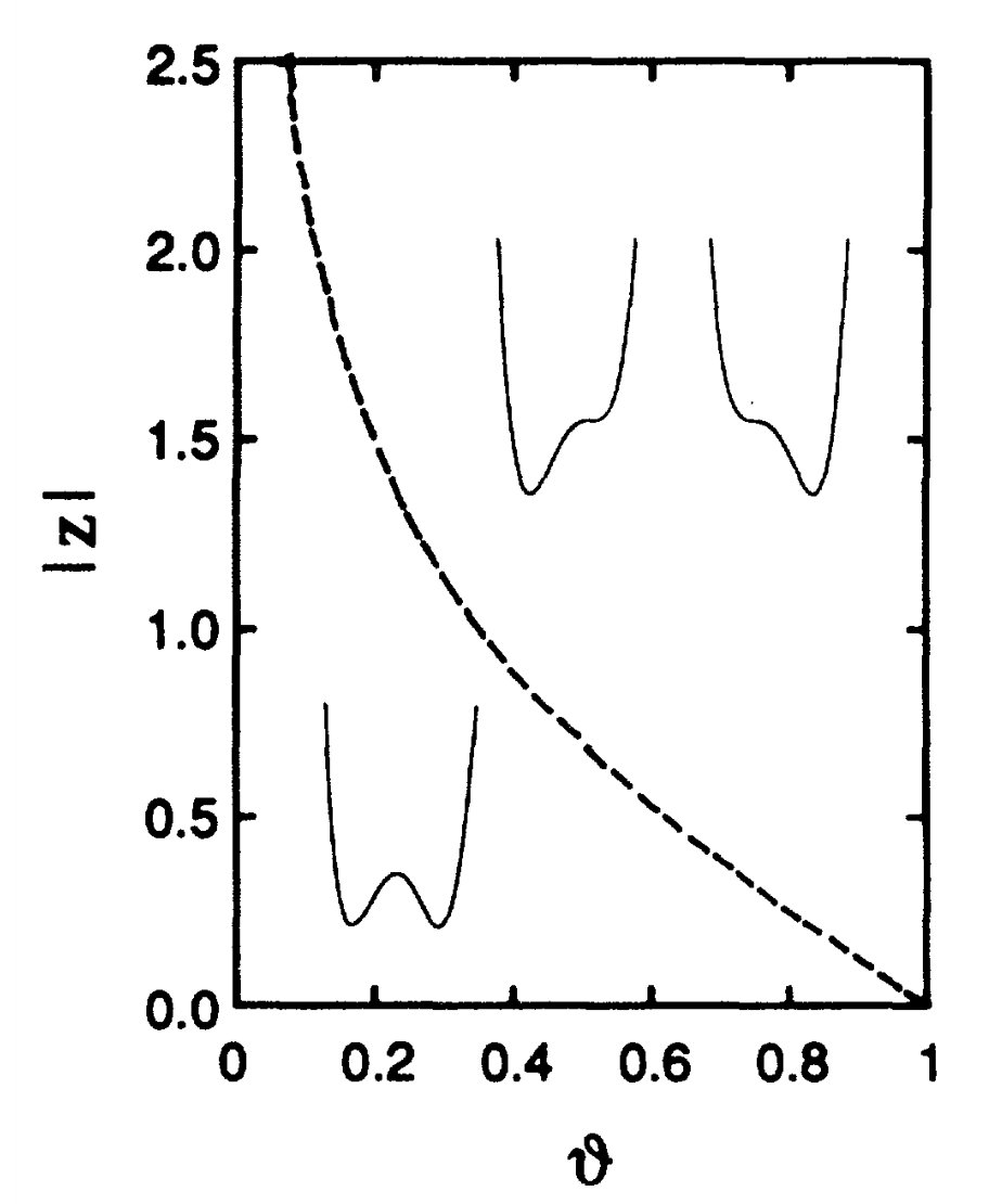 Figure 1
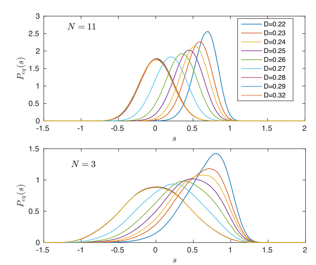 Figure 2
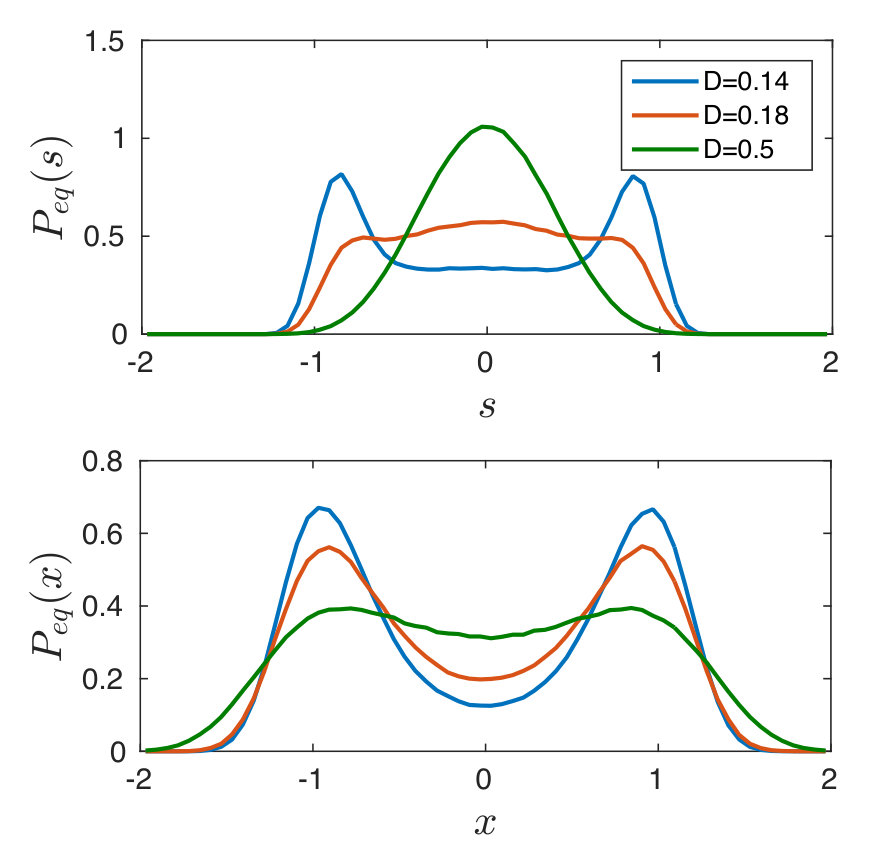 Figure 3
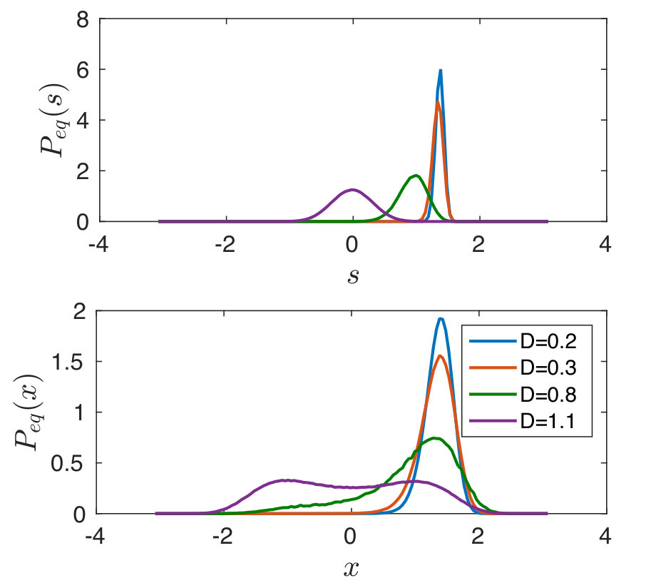 Figure 4
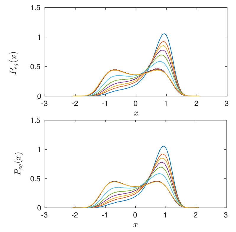 Figure 5
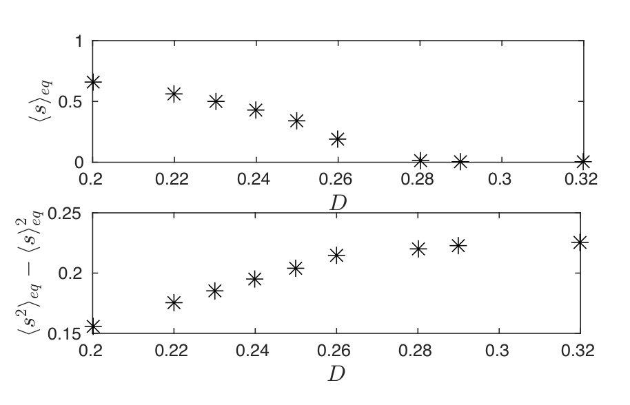 Figure 6
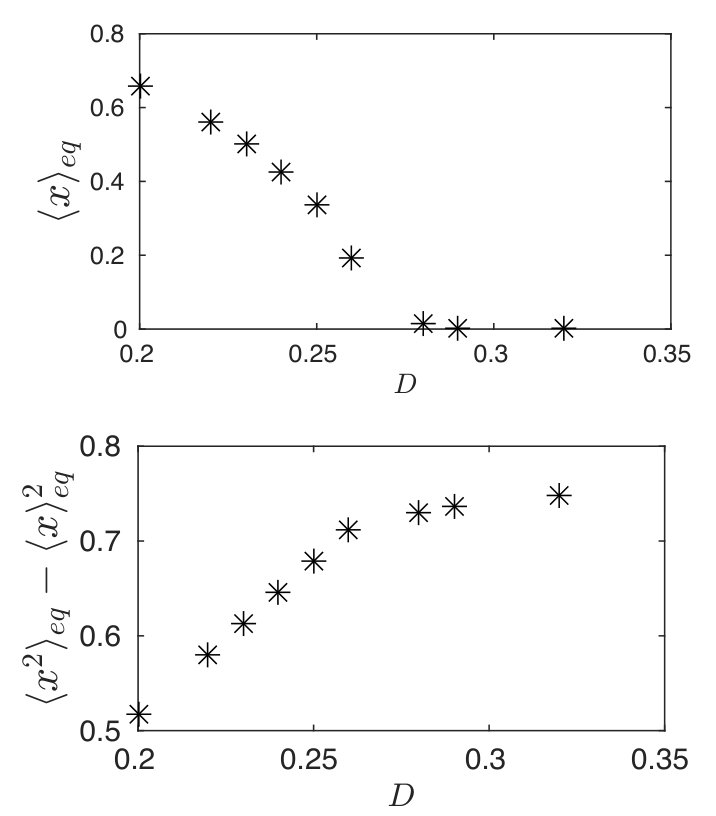 Figure 7
Peer Reviews
No public reviews on file for this paper yet. If you reviewed it on a platform where reviews are public (OpenReview, ICLR, NeurIPS, ICML), you can paste yours below so the community can read it here.
Videos
No videos yet. Explain this paper in a talk, walkthrough, or lecture? Add one.
Taxonomy
TopicsStochastic processes and statistical mechanics · Mathematical Biology Tumor Growth · Complex Systems and Time Series Analysis
Behavior of collective variables in complex nonlinear stochastic models of finite size
M. Morillo and J. M. Casado
Area de Física Teórica. Universidad de Sevilla.
Apartado Correos 1085, 41080 Sevilla (Spain)
Abstract
We consider the behavior of a collective variable in a complex system formed by a finite number of interacting subunits. Each of them is characterized by a degree of freedom with an intrinsic nonlinear bistable stochastic dynamics. The lack of ergodicity of the collective variable requires the consideration of a feedback mechanism of the collective behavior on the individual dynamics. We explore numerically this issue within the context of two simple finite models with a feedback mechanism of the Weiss mean-field type: a global coupling model and another one with nearest neighbors coupling.
I Introduction
Complex hierarchical systems admit several levels of description. At a microscopic level, the interest lies on the dynamical behavior of the constituent elements. Thus, at this level of description, one needs to follow the time evolution of very many microscopic variables. On the other hand, at the macroscopic level, one describes the system in terms of just a few collective variables characterizing it as a whole. The laws describing the behavior of collective variables could, in principle, be deduced from the dynamical laws governing the elementary constituents. In practice this is not an easy task as, in general, the dynamical equations for the collective variables can not be obtained from the microscopic dynamics without further approximations. On the other hand, in general, when studying a complex systems, there are just the collective variables which are accessible to experimental measurements. The detailed dynamics of the constituent elements has to be inferred from the information about the collective variables.
A fundamental property common to all complex systems made of a collection of interacting elements (subsystems) is the existence of feedback mechanisms of the whole system behavior into the dynamics of the subsystems KOMETANI1975 . The evolution of the system is determined by those of its elements in a statistical way and, at the same time, the feedback loops put the subsystems under the control of the global system. Such feedback loops, for example, give rise to the biological laws that characterize the phenomenon of life. In fact, this mutual interlevel control introduces a self-regulation mechanism to the dynamics of the hierarchical system against external forces and boundary conditions.
In this work, we have studied two very simple models describing a finite system composed of several subsystems. Each of them is characterized by a single stochastic variable . The subsystems have an intrinsic nonlinear bistable dynamics and they are coupled among them either in a global or local form. The whole system is characterized by a collective variable. We will assume that the information about the system comes from the observation of the collective variable. The randomness of the subsystem variables is due to a noise term in their dynamics. We will take this noise to be a white Gaussian noise characterized by a noise parameter . This noise can originate for instance, from the weak interactions between the subsystems and a large thermal bath with a temperature .
A goal of this work is to study the form of the distribution function for the collective variable and to compare it with the distribution function of a single element for small finite systems. As we will see, in the absence of feedback, both distributions are unique, regardless of the initial preparation of the system. This is a consequence of the fact that the joint probability distribution satisfies a linear Fokker-Planck equation. If the observations of the collective variable are compatible with such a behavior, then we can accept the microscopic description.
But, if one observes that, depending upon the noise value and the strength of the subsystems coupling, the equilibrium distribution might not be unique and it might depend on the initial preparation of the system, then the linear Fokker-Planck equation (or equivalently, the set of coupled Langevin-like equations) is not adequate. To deal with such a situation, we propose stochastic dynamics leading to nonlinear Fokker-Plank equations. The idea is simply an extension of the old Weiss mean-field approach to the equilibrium properties of magnetic systems. Then, as the system parameters are varied, the dynamics leads us from just a single stationary solution to situations where two distributions are stable and the system goes to one or the other depending upon the initial conditions.
We should point out that such a non-uniqueness of a single variable distribution function was studied long ago by several authors DESAI1978 ; DAWSON1983 ; SHIINO . They were able to derive a nonlinear Fokker-Planck equation for a single variable in the limit of an infinite system. We emphasize that, in this work, we are interested in small, finite systems.
The intrinsic bistable nonlinearity of the subsystems dynamics forbids explicit analytical solutions, but it is essential for the behavior indicated above. A closed, explicit, stochastic evolution equation for the collective variable can not be found from the subsystems dynamics. We will then rely on numerical simulations of the stochastic evolution equations for the subsystems variables.
II Two stochastic nonlinear models
II.1 A model with global interactions
We consider a system formed by a set of subsystems each one described by a single stochastic variable , whose dynamics is given by the coupled Langevin equations (in dimensionless form)
[TABLE]
where is the strength of the coupling and are Gaussian white noises with
[TABLE]
This model was introduced some years ago by Kometani and Shimizu KOMETANI1975 in a biophysical context and was later analyzed by Desai and Zwanzig DESAI1978 and Dawson DAWSON1983 from a more general statistical mechanical perspective. An alternative formulation can be casted in terms of the linear Fokker-Planck equation for the joint probability distribution ,
[TABLE]
where is the potential energy relief,
[TABLE]
with the single particle potential
[TABLE]
In the limit , one can write a Nonlinear Fokker-Planck Equation (NLFPE) for the one particle probability distribution, DESAI1978 ; DAWSON1983 ; SHIINO ; FRANK ; KURSTEN2016
[TABLE]
where
[TABLE]
In this limit, the system undergoes an order-disorder phase transition signaled by a change in the form of the equilibrium one-particle probability distribution and by the fact that for some values of the parameters and , the ergodicity is broken and there are more than one stable equilibrium distribution. The system ends up in one of them depending on its initial preparation. In Fig. 1 we sketch different regions in the parameter space and , separated by a transition line. Below the transition line, there is just one single distribution, regardless of the initial preparation of the system, leading to a single equilibrium with two maxima. This is indicated in the figure by drawing a double well potential. On the other hand, above the transition line, two stable monomodal equilibrium distributions are possible. Depending upon the initial condition the system relaxes to one or the other. This feature is illustrated in the figure by drawing two asymmetrical single minima potentials.
Let us define a collective variable
[TABLE]
Then, the Langevin equations (1) can be casted in the equivalent form
[TABLE]
The nonlinearity of equations (9) prevent us from writing a closed Langevin equation for . Note that there is a feedback of the collective dynamics in the Langevin dynamics of each degree of freedom. But, as we analyzed in a previous work GOMEZ2009 , with this type of feedback for the finite model the single variable distribution is unique for any set of parameter values. This is consistent with the fact that the joint probability distribution satisfies a linear Fokker-Plank equation with a unique distribution function for any values of the parameters.
We now propose to replace the model with
[TABLE]
Here, represents a noise average of the collective variable defined in Eq. (8). Clearly, the Langevin equation, Eq. (10) has to be solved concurrently with the evaluation of this average. The proposal amounts to replace in the dynamical evolution of each individual degree of freedom the whole stochastic process by its noise average, in the spirit of Weiss mean-field approximation to magnetism. Note that within this model, the collective variable is itself a fluctuating quantity, even though just its average value influences the subsystems dynamics.
II.2 A model with nearest neighbors interactions
This model is described by the (dimensionless) set of Langevin equations
[TABLE]
with the periodic conditions and . The noises are white Gaussian with the properties given in Eq. (2). As in the global interaction model, the joint probability distribution function satisfies a linear Fokker-Planck equation similar to the one in Eq. (3) but with the potential energy relief,
[TABLE]
Then, also for this case, the joint probability distribution satisfies a linear Fokker-Plank equation with a unique distribution function for any values of the parameters.
As in the global interaction case, we will now replace Eq. (11) with
[TABLE]
As said above, in both situations, even after using the Weiss approach, the collective variable for finite is still a random process with a probability distribution defined by
[TABLE]
Notice that within the mean field dynamics, the joint probability distribution factorizes as a product of single particle distributions, each of them satisfying a NLFPE similar to the one in (6) for the single particle distribution in the infinite size limit.
Defining the characteristic function of a distribution as
[TABLE]
one can easily see that the generating function of the collective variable and that of a single particle variable are related by
[TABLE]
Thus, the corresponding cumulant generating functions are related by . Then, the cumulants associated to the stochastic process , and those associated to the process, are related by
[TABLE]
In the limit of very large , becomes a very narrow peak around its first moment as indicated in DESAI1978 ; DAWSON1983 ; SHIINO .
III Numerical procedure
We have solved numerically the corresponding Langevin equations, Eqs. (9,11) and Eqs.(̃10,13) for systems with a small number of subsystems using very many noise realizations. The numerical method used has been detailed elsewhere our . After a convenient relaxation time so that the equilibrium probability distributions have been reached, we construct histograms that approximate the equilibrium probability distributions and .
Notice that the generation of Langevin trajectories for all the degrees of freedom for the mean field dynamics requires the knowledge of . Thus, at each time step during the evolution, this noise average is evaluated from the instantaneous values of each subsystem variable for each realization of the noise. Namely,
[TABLE]
where is the number of noise realizations considered.
Let us first consider the case of global coupling with mean-field dynamics. In Fig. 2 we depict the equilibrium distribution of the collective variable for several values of the noise strength and two system sizes, (upper panel) and (lower panel). In all cases, we have used and initial conditions such that . As seen in the figure, the qualitative behavior is quite independent of , except for the narrowing of the distribution as increases. For the parameter values considered, is always monomodal, with a peak that is displaced from to higher values of as the noise is decreased. Note that the peak is located at positive values of because, at the initial time, we located the value of to be positive. Had we started from the same initial values, but with a negative sign, the plots for would be as in Fig. 2, but with the peaks located at negative values.
In Fig. 3, we depict the equilibrium distribution for a single variable for several values of the noise strength and for two systems with (upper panel) and (lower panel). In all cases, we have used . Again, the qualitative behavior is quite independent of . By contrast with the behavior of , the single variable distribution changes its shape from a bimodal distribution centered at to a monomodal one, with a peak that is displaced to nonzero values of as the noise is decreased.
In Figs. 4 and 5 we depict the behavior of the equilibrium first and second cumulant moments of the collective variable and that of an individual variable for a system with degrees of freedom and mean-field global dynamics. The parameter values are indicated in the captions. The average values have been obtained from the corresponding numerical integration involving the equilibrium histograms constructed from the Langevin simulations. As expected from Eq. (15), the first moment of the individual and the collective variables are the same, while the second cumulant for the collective variable is smaller than that of the individual one. For the parameter values used in these figures, the probability distribution centered at (or ) is unstable for smaller than a bifurcation value. In the figures we have just depicted that branch of the stable first moments which are reached from the imposed initial condition .
The case of nearest neighbors interactions is qualitatively similar to the case of global interactions. We will just depict as an example the contrast in the behavior of for the finite model in Eq. (11) and the corresponding one with the mean field dynamics Eq. (13). In Fig. 6 we plot the behavior of and for a system with and nearest neighbors coupling. In Fig. 7 the same distributions are sketched but now with the systems described by the mean-field dynamics. In both dynamics there is a change in the shape of the equilibrium distribution as the noise value is varied. But for the finite case described by Eq. (11) the equilibrium distribution is always unique regardless of the initial preparation. On the other hand, the mean field dynamics leads to a bifurcation of the distribution as is varied. For large values of there is a single stable . As is decreased while keeping constant, the zero centered distribution becomes unstable and two stable distributions appear with peaks located at or depending on the initial preparation.
IV Conclusions
We have carried out numerical simulations to study some aspects of the behavior of complex stochastic systems formed by a finite number of subsystems with bistable intrinsic dynamics and mean field couplings. We have contrasted the behavior of each individual degree of freedom with that of a collective variable characterizing the entire system.
The systems considered have finite sizes. Then, the collective variable is also a stochastic variable with a probability density with a finite width, in contrast with what occurs in the infinite size limit. Furthermore, the mean field dynamics is compatible with the possible existence of several probability distributions in some regions of the parameter space. There is a transition from a single stable distribution to the several stable ones as the noise strength is varied for a fixed value of the coupling parameter. In the case of multiple distributions, the one that is observed depends upon the initial preparation.
We argue that if the stochastic collective variable is the accessible one, and it is such that its average value depends upon the initial conditions, the modelling of the subsystems dynamics requires the introduction of some sort of feedback of the average collective behavior on the individual dynamics. An example of this feedback is the mean field dynamics considered in this paper. It should be pointed out that in order to have the above mentioned transition between one or several distributions, the intrinsic bistable dynamics of each individual degree of freedom is essential.
The reference list from the paper itself. Each links out to its DOI / PubMed record.
- 1(1) K. Kometani and H. Shimizu, J. Stat. Phys. 13 , 473 (1975).
- 2(2) R. C. Desai and R. Zwanzig, J. Stat. Phys. 19 , 1 (1978).
- 3(3) D. A. Dawson, J. Stat. Phys. 31 , 29 (1983).
- 4(4) M. Shiino, Phys. Rev. A 36 ,2393 (1986).
- 5(5) T. D. Frank, Nonlinear Fokker-Planck equations. Fundamentals and Applications, Springer, (2005).
- 6(6) R. Kürsten, U. Behn, Phys. Rev. E 94 , 062135 (2016).
- 7(7) J. Gómez-Ordóñez, J. M. Casado, M. Morillo, C. Honisch, and R. Friedrich, Europhys. Lett. 88 400006 (2009).
- 8(8) M. Morillo,J. Gómez-Ordóñez, and J. M. Casado, Phys. Rev. E 52 ,316 (1995).