Algorithms for outerplanar graph roots and graph roots of pathwidth at most 2
Petr A. Golovach, Pinar Heggernes, Dieter Kratsch, Paloma T. Lima, and, Daniel Paulusma

TL;DR
This paper presents polynomial-time algorithms to determine if a graph has an outerplanar square root or a square root with pathwidth at most 2, addressing a classical NP-complete problem in specific graph classes.
Contribution
It introduces new polynomial-time algorithms for deciding the existence of outerplanar and pathwidth at most 2 square roots of a given graph.
Findings
Polynomial-time algorithm for outerplanar square root recognition
Polynomial-time algorithm for square root with pathwidth at most 2
Advances understanding of graph root problems in restricted classes
Abstract
Deciding whether a given graph has a square root is a classical problem that has been studied extensively both from graph theoretic and from algorithmic perspectives. The problem is NP-complete in general, and consequently substantial effort has been dedicated to deciding whether a given graph has a square root that belongs to a particular graph class. There are both polynomial-time solvable and NP-complete cases, depending on the graph class. We contribute with new results in this direction. Given an arbitrary input graph G, we give polynomial-time algorithms to decide whether G has an outerplanar square root, and whether G has a square root that is of pathwidth at most 2.
Click any figure to enlarge with its caption.
 Figure 1
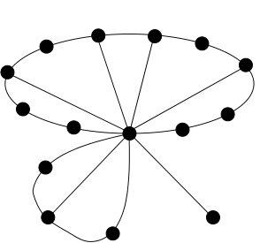 Figure 2
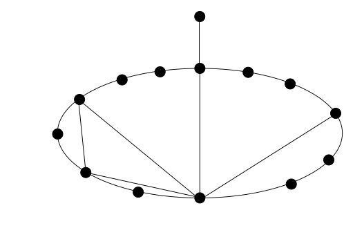 Figure 3
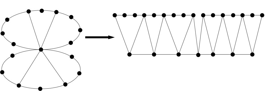 Figure 4
Peer Reviews
No public reviews on file for this paper yet. If you reviewed it on a platform where reviews are public (OpenReview, ICLR, NeurIPS, ICML), you can paste yours below so the community can read it here.
Videos
No videos yet. Explain this paper in a talk, walkthrough, or lecture? Add one.
Algorithms for Outerplanar Graph Roots
and Graph Roots of Pathwidth at Most ††thanks: This paper received support from the Research Council of Norway via the project “CLASSIS” and the Leverhulme Trust via Grant RPG-2016-258. An extended abstract of it appeared in the proceedings of WG 2017 [16].
Petr A. Golovach Department of Informatics, University of Bergen, PB 7803 N-5020 Bergen, Norway, {petr.golovach,pinar.heggernes,paloma.lima}@uib.no
Pinar Heggernes00footnotemark: 0
Dieter Kratsch Université de Lorraine, LITA, Metz, France, [email protected]
Paloma T. Lima-1-1footnotemark: -1
Daniël Paulusma Department of Computer Science, Durham University, Durham DH1 3LE, UK, [email protected]
Abstract
Deciding if a graph has a square root is a classical problem, which has been studied extensively both from graph-theoretic and algorithmic perspective. As the problem is NP-complete, substantial effort has been dedicated to determining the complexity of deciding if a graph has a square root belonging to some specific graph class . There are both polynomial-time solvable and NP-complete results in this direction, depending on . We present a general framework for the problem if is a class of sparse graphs. This enables us to generalize a number of known results and to give polynomial-time algorithms for the cases where is the class of outerplanar graphs and is the class of graphs of pathwidth at most .
1 Introduction
Squares and square roots of graphs form a classical and well-studied topic in graph theory, which has also attracted significant attention from the algorithms community. A graph is the square of a graph if and have the same vertex set, and two vertices are adjacent in if and only if the distance between them is at most in . This situation is denoted by , and is called a square root of . A square root of a graph need not be unique; it might even not exist. That is, there are graphs without square roots, graphs with a unique square root, and graphs with several different square roots. Characterizing and recognizing graphs with square roots has therefore been an intriguing and important graph-theoretic problem for more than 50 years (see e.g. [15, 32, 35]).
In 1967, Mukhopadhyay [32] proved that a graph on vertex set has a square root if and only if contains complete subgraphs , such that each contains , and vertex belongs to if and only if belongs to . Unfortunately, this characterization does not yield a polynomial-time algorithm for deciding whether has a square root. This problem is called the Square Root problem. In 1994, Motwani and Sudan [31] proved that Square Root is NP-complete.
Motivated by its computational hardness, special cases of Square Root have been studied where the input graph belongs to a particular graph class. It is known that Square Root is polynomial-time solvable on planar graphs [28], and more generally, on every non-trivial minor-closed graph class [33]. Polynomial-time algorithms also exist if the input graph belongs to one of the following graph classes: block graphs [26], line graphs [29], trivially perfect graphs [30], threshold graphs [30], graphs of maximum degree 6 [7], graphs of maximum average degree smaller than [18]111The average degree of a graph is defined as . The maximum average degree of is then defined as . graphs with clique number at most 3 [18], and graphs with bounded clique number and no long induced path [18]. On the negative side, Square Root is NP-complete on chordal graphs [23]. There also exist a number of parameterized complexity results for the problem [8, 19].
The intractability of Square Root has also been attacked by restricting properties of the square root. In this case, the input graph is an arbitrary graph, and the question is whether has a square root that belongs to some graph class specified in advance. This problem is called -Square Root, and this is the problem which we focus on in this paper.
Significant advances have also been made on the complexity of -Square Root. Previous results show that -Square Root is polynomial-time solvable for the following graph classes : trees [28], proper interval graphs [23], bipartite graphs [22], block graphs [26], strongly chordal split graphs [27], ptolemaic graphs [24], 3-sun-free split graphs [24], cactus graphs [18], cactus block graphs [12] and graphs with girth at least for any fixed [14]. The result for 3-sun-free split graphs was extended to a number of other subclasses of split graphs in [25]. We observe that if -Square Root is polynomial-time solvable for some class , then this does not automatically imply that -Square Root is polynomial-time solvable for a subclass of .
On the negative side, -Square Root remains NP-complete for each of the following classes : graphs of girth at least 5 [13], graphs of girth at least 4 [14], split graphs [23], and chordal graphs [23]. All known NP-hardness constructions involve dense graphs [13, 14, 23, 31], and the square roots that occur in these constructions are dense as well. This, in combination with the aforementioned polynomial-time results, leads to our underlying research question:
Is -Square Root polynomial-time solvable for every sparse graph class ?
Our Results
We give further evidence for the above question by proving that -Square Root is polynomial-time solvable for two classes , namely when is the class of outerplanar graphs, and when is the class of graphs of pathwidth at most . Both classes are well studied. In particular, Syslo [36] characterized outerplanar graphs by a list of two forbidden minors, and Kinnersley and Langston [21] gave a characterization of graphs of pathwidth at most 2 by a list of 110 forbidden minors (see [1, 2] for an alternative approach). Outerplanar graphs have treewidth at most 2 [3]. However, they can have arbitrarily large pathwidth (as every tree is outerplanar and trees can have arbitrarily large pathwidth). Moreover, there exist graphs of pathwidth at most 2 that are not outerplanar; take, for instance, the complete bipartite graph on vertices for any .
The proofs of our results rely on structural properties that are specific for outerplanar graphs or graphs of pathwidth at most 2, respectively. However, despite the fact that the two classes are incomparable, the approach to obtain polynomial-time algorithms for each of them is based on the same general framework. The basic idea is to use appropriate polynomial-time reduction rules, in which we try to recognize edges of the input graph that belong to any square root or to no square root of at all. The goal is to obtain a graph whose treewidth is bounded by a constant, which enables us to solve the problem in polynomial time after expressing it in Monadic Second-Order Logic and applying a classical result of Courcelle [9]. This idea has been used before (see, for instance, [7, 8, 18, 19]), but in this paper we formalize the idea into a general framework. We discuss this framework in detail in Section 3.
Sections 4 and 5 are dedicated to outerplanar graphs and graphs of pathwidth at most 2, respectively. In each of these two sections, we first prove the necessary structural properties of the graph class followed by a description of the algorithm, proof of correctness and running time analysis. Afterwards we prove that our general framework enables us to solve -Square Root in polynomial time for every subclass of outerplanar graphs or graphs of pathwidth at most 2, respectively, that satisfies the following two conditions:
- (i)
is closed under taking a subgraph, and
- (ii)
can be defined in Counting Monadic Second-Order Logic.
To give a few examples, our results imply the aforementioned results for the cases where is the class of forests [28] or cactus graphs (graphs in which every edge belongs to at most one cycle) [18], which both are subclasses of outerplanar graphs that satisfy conditions (i) an (ii). To give another example, a connected graph has pathwidth 1 if and only if it is a caterpillar (a tree which can be modified in a path after removing all vertices of degree 1). The problem of deciding if a graph has a square root that is a caterpillar can be solved in polynomial time via a straightforward adaptation of the algorithm of [28, 35] for trees. As the class of unions of caterpillars satisfy conditions (i) and (ii), this also follows from our results. Moreover, graphs of bandwidth at most 2, or equivalently, graph of proper pathwidth at most 2 [20] have pathwidth at most 2 and satisfy conditions (i) and (ii). Hence we can also recognize squares of such graphs in polynomial time due to our results.
2 Preliminaries
We consider only finite undirected graphs without loops and multiple edges. We refer to the textbook by Diestel [11] for any undefined graph terminology. In the remainder we let be a graph.
We denote the vertex set of by and the edge set by . We use to denote the number of vertices of a graph (if this does not create confusion). The subgraph of induced by a subset is denoted by . The graph is the graph obtained from after removing the vertices of . If , we also write . Similarly, we denote the graph obtained from by deleting a set of edges , or a single edge , by and , respectively.
The distance between a pair of vertices is the number of edges of a shortest path between them in . We write for a set of vertices . For a positive integer and , we write . For , we write instead of and say that is the open neighborhood of . The closed neighbourhood of a vertex is defined as . For , we let . Two distinct vertices are said to be true twins if and are false twins if . A vertex is simplicial if is a clique, that is, if there is an edge between any two vertices of . The degree of a vertex is defined as . The maximum degree of is . A vertex of degree 1 is said to be a pendant vertex of .
Let denote the complete graph on vertices and the complete bipartite graph with partition classes of size and , respectively.
A (connected) component of is a maximal connected subgraph. A vertex is a cut vertex of a graph if has more connected components than . A connected graph without cut vertices is said to be biconnected. An inclusion-maximal induced biconnected subgraph of is called a block of .
The contraction of an edge of a graph is the operation that deletes the vertices and and replaces them by a vertex adjacent to every vertex of . A graph is a contraction of a graph if can be obtained from by edge contractions. A graph is a minor of if can be obtained from by vertex deletions, edge deletions and edge contractions.
The syntax of Monadic Second-Order Logic (MSO) on graphs includes
- •
logical connectivities , and ,
- •
variables for vertices, edges, sets of vertices and sets of edges,
- •
the quantifiers and that apply to variables,
- •
the predicates , , and for equality, inclusion of an element in a set, adjacency of vertices and incidence of a vertex with an edge, respectively.
Counting Monadic Second-Order Logic (CMSO) is the extension of MSO with the predicate defined on sets for some integer constants and with and , such that if and only if . For a CMSO formula on graphs, we write to denote that evaluates on . We refer to the book of Courcelle and Engelfriet [10] for an introduction to MSO and CMSO.
We will use the following well-known fact (see, for example, [10]).
Lemma 1**.**
The property that a graph contains a fixed graph as a minor can be expressed in MSO.
2.1 Square Roots
For a positive integer , the -th power of a graph is the graph with vertex set , such that every pair of distinct vertices and of are adjacent if and only if . If , then is called a square of , and is called a square root of if .
We say that a square root of a graph is minimal if no proper subgraph of is a square root of . We need two basic lemmas on minimal square roots. The first lemma follows immediately from the definition. We give a short proof for the second lemma.
Lemma 2**.**
Let be a graph class closed under taking edge deletions and vertex deletions. If a graph has a square root in , then has a minimal square root in .
Lemma 3**.**
Let be a minimal square root of a graph that contains three vertices that are pairwise adjacent in . Then or has a neighbour in such that is not adjacent to in and is adjacent to exactly one of in .
Proof.
As is a minimal square root of , is not a square root of . Hence, there is an edge , such that has a unique -path of length and is an edge of this path. Therefore, exactly one of is adjacent to in . As and are both edges in , this means that or for some . Note that is not adjacent to , because, otherwise, either or would be the second -path of length 2. ∎
We also need a lemma that is implicit in [18]. This lemma enables us to identify some edges that are not included in any square root.
Lemma 4**.**
Let be two neighbours of a vertex in a graph that are of distance at least in . Then for any square root of .
Proof.
Suppose is a square root of . For contradiction, assume . If , then contradicting the assumption that . Hence . As , there exists a vertex such that . If , then ; a contradiction. If , then and imply that . Hence is a path in of length 2, and again we obtain a contradiction with our assumption that . We conclude that and for the same reason we obtain . ∎
2.2 Treewidth and Pathwidth
A tree decomposition of a graph is a pair where is a tree, whose vertices are called nodes, and is a collection of subsets, called bags, of such that the following three conditions hold:
- i)
;
- ii)
for all , for some ; and
- iii)
for all , induces a connected subtree of .
The width of a tree decomposition is . The treewidth of a graph is the minimum width over all tree decompositions of . If is a path, then we say that is a path decomposition of . The pathwidth of is the minimum width over all path decompositions of . Notice that a path decomposition of can be seen as a sequence of bags. We always assume that the bags are distinct and inclusion incomparable, that is, there are no bags and such that .
The next lemma gives two fundamental results on treewidth and pathwidth, which are due to Bodlaender, and Bodlaender and Kloks, respectively.
Lemma 5** ([4, 5]).**
For every constant , it is possible to decide in linear time whether the treewidth or the pathwidth of a graph is at most .
We will also need the following two well-known lemmas. We refer to [11] for the first lemma. Note that this lemma also holds if is a contraction of (as this immediately implies that is a minor of ). We provide a proof of the second lemma. This lemma is also folklore, but might not have been stated in this way. In particular, we formulate it for arbitrary instead of for only, as we will need this observation in general form to prove our results.
Lemma 6**.**
Let and be graphs. If is a minor of , then and .
Lemma 7**.**
For a graph and an integer , the following hold: and
Proof.
We show that . The proof of the second inequality uses the same arguments. The inequality is trivial if or . Assume that and . Let also .
Let be a tree decomposition of of minimum width. For , we define and . We show that is a tree decomposition of by proving that conditions (i)–(iii) of the definition of treewidth are satisfied.
(i). As for all , we obtain , so . As , this means that , so (i) holds.
(ii). Consider an edge of . By the definition of , contains a -path of length at most . Then has an edge such that and . Because is a tree decomposition of , there is a node such that . We find that . Hence (ii) holds.
(iii). For contradiction, assume that there is such that the set is disconnected. Then there exist two distinct nonadjacent nodes such that , , and for every internal node of the unique -path in . Since , there exists a vertex such that . Similarly, there exists a vertex such that . Let and be shortest -paths and -paths in respectively. Then contains an -path whose edges belong to . Note that every vertex of is of distance at most from in .
Consider an arbitrary internal node of the unique -path in . Let . As , it follows that . Hence, . We conclude that . This means that the bag does not separate and in , which contradicts a basic property of a tree decomposition (see, for example, Lemma 12.3.1 [11]).
We now prove the bound on the width of . For , we find that
[TABLE]
Hence . ∎
We will also need the following characterization of graphs of pathwidth at most , which is due to Kinnersley and Langston (we do not specify the graphs on their list, as this is irrelevant for our purposes).
Lemma 8** ([21]).**
A graph has pathwidth at most if and only if does not contain a graph from a specific list of 110 graphs as a minor.
As mentioned we will also need the following classical result of Courcelle as a lemma.
Lemma 9** ([9]).**
For every fixed integer and every problem expressible in CMSO, there exists a linear-time algorithm that solves for the class of graphs of treewidth at most .
2.3 Outerplanar Graphs
A graph is planar if admits a planar embedding, which is an embedding on the plane in such a way that the edges of only intersect at their end-points. A planar graph is outerplanar if it admits a planar embedding in which all its vertices belong to the outerface. When considering an outerplanar graph, we always assume that such an embedding is given.
If is a planar biconnected graph different from , then for any of its embeddings, the boundary of each face is a cycle (see, e.g., [11]). If is a biconnected outerplanar graph distinct from , then the cycle forming the boundary of the external face is unique [36]. We call the boundary cycle of . Every vertex of belongs to , and every edge of is either an edge of or a chord of , that is, its endpoints are vertices of that are non-adjacent in . By definition, these chords are not intersecting in the embedding. We define the clockwise ordering of with respect to some vertex of as the clockwise ordering of the vertices on starting from . For a subset of vertices , the clockwise ordering of with respect to is the restriction of the clockwise ordering of to the vertices of . See Figure 1 for an example of these notions.
We use the above terms for blocks of an outerplanar graph that are distinct from . We say that two distinct vertices are consecutive with respect to if and are in the same block of and there are no vertices of between and in the clockwise ordering of the vertices of the boundary cycle of with respect to . For a set of vertices , we say that the vertices of are consecutive with respect to if the vertices of are in the same block of and any two vertices of consecutive in the clockwise ordering of the vertices of with respect to are consecutive with respect to . See Figure 2 for an illustration of these notions.
Sysło characterized the class of outerplanar graphs via a set of two forbidden minors.
Lemma 10** ([36]).**
A graph is outerplanar if and only if it does not contain or as a minor.
We will also need the following well-known result.
Lemma 11** ([3]).**
Every outerplanar graph has treewidth at most .
3 General Algorithmic Approach
Our algorithms for deciding whether a graph has an outerplanar square root or a square root that has pathwidth at most 2, respectively, rely on similar ideas and concepts.
The framework underlying these two algorithms is general and has the potential to be applicable to find other restricted square roots as well. This section is devoted to explain this framework.
We observe that even though outerplanar graphs and graphs of pathwidth at most 2 have bounded treewidth, squares of such graphs may have arbitrarily large treewidth. The basic idea is to reduce an input graph of our problem in polynomial time to a graph of bounded treewidth that is an instance of a closely related auxiliary problem. After showing that this auxiliary problem can be expressed in MSO, we can then apply the well-known result of Courcelle [9].
Let be the class of outerplanar graphs or graphs of pathwidth at most 2. Let be the input graph. In order to find out if has a square root , we modify using the following polynomial-time rules, which we apply exhaustively in the order below:
Deleting irrelevant vertices. We try to identify vertices that can be deleted from , such that the resulting graph has a square root that belongs to if and only if has a square root that belongs to . If is the class of outerplanar graphs, then this step allows us to bound the number of true twins of a simplicial vertex of . If is the class of graphs of pathwidth at most 2, then this step allows us to bound the number of true twins of a vertex of . 2. 2.
Labeling edges. We try to identify edges in that we can give a specific label. That is, we label an edge of red if we can determine that belongs to every minimal square root of and we label blue if we can determine that does not belong to any minimal square root of . We let and denote the sets of red and blue edges, respectively. 3. 3.
Deleting irrelevant edges. We determine a set such that for each , all edges incident to are labeled either red or blue. We return a no-answer if there exist two red edges that form an induced path of length 2 in . Otherwise, for each , we identify a set of edges in that we may remove from . The crucial properties of every deleted edge are that (i) is not included in any minimal square root of and (ii) there are two red edges incident to in that form an -path.
After performing each of these three rules exhaustively in the given order, we obtain a new graph . The crucial point here is that if the treewidth of is greater than some constant that does not depend on or , then does not have a square root such that . Assume that the treewidth of is at most . Recall that in order to obtain we deleted some edges of . Therefore, a square root of is not necessarily a square root of and, moreover, may not even have a square root. Nevertheless, by using properties (i) and (ii) above, we can recover the structure of a square root of . More formally, we prove that has a square root in if and only if contains a subset with the following properties:
- (i)
and ;
- (ii)
for every , or there exists a vertex with ;
- (iii)
for every two distinct edges , or there is a vertex with ; and
- (iv)
the graph belongs to .
In fact, is a square root of the graph obtained from via exhaustive application of the first rule. Since has bounded treewidth and properties (i)–(iv) can be expressed in MSO, we can test the existence of the set in polynomial time by applying the aforementioned result of Courcelle [9].
4 Outerplanar Roots
We say that a square root of is an outerplanar root if is outerplanar, and we define the following problem:
Outerplanar Root
* Instance:*
a graph .
Question:
does have an outerplanar root?
The main result of this section is the following theorem.
Theorem 1**.**
Outerplanar Root* can be solved in time.*
We first show a number of structural results in Section 4.1. We then use these results in the design of our polynomial-time algorithm for Outerplanar Root in Section 4.2.
4.1 Structural Lemmas
As the class of outerplanar graphs is closed under vertex an edge deletions, we may restrict ourselves to minimal outerplanar roots by Lemma 2.
We start with the following lemmas.
Lemma 12**.**
Let be a minimal square root of a graph , and let . If is not a pendant vertex of , then there is a vertex that is adjacent to in .
Proof.
Since is not a pendant vertex of , has at least one neighbour in distinct from . If there exists a vertex such that , then the claim holds. Assume that for every distinct from , it holds that . Consider such a neighbour . By Lemma 3, or has a neighbour in such that . By our assumption on , we find that this vertex cannot be and thus must be . Since , we find that . Hence is adjacent to in , as desired. ∎
Let be a minimal square root of a graph and let . We define the following set:
[TABLE]
We use to detect edges with both endpoints in that are excluded from every minimal square root of .
Lemma 13**.**
Let be a minimal square root of a graph , and let . If for two distinct vertices there is no set such that , then .
Proof.
Suppose that for two distinct vertices , . By Lemma 3, there is a vertex such that is adjacent to or in , but is not adjacent to in . We find that and are adjacent to in and, therefore, . In other words, . ∎
We need the following two lemmas about the structure of for minimal outerplanar roots.
Lemma 14**.**
Let be a minimal outerplanar root of a graph , and let . Then, for each , is consecutive with respect to .
Proof.
Let and consider a vertex such that . As but , we find that must be adjacent to a vertex of . Hence .
If , then the claims holds by definition. Assume that .
We first observe that the vertices of are in the same block of . This can be seen as follows. Suppose are two vertices that are not in the same block of . Then any vertex adjacent to and in must belong to . Hence , which is not possible.
Let be the boundary cycle of . Assume that and that the vertices are numbered in the clockwise order with respect to . Suppose that is not consecutive with respect to . Then, by definition, there exists a vertex that lies on between two vertices and for some , such that does not belong to . The latter implies that . Since and belong to by definition of , we find that has an -path and an -path , each of length at most . The paths and do not contain , due to the facts that and the length of and is at most . Moreover, and do not contain , as and both paths have length at most .
Let be the subpath of from to that does not contain , and let be the subpath of from to that does not contain . First suppose that does not belong to or . We contract all edges on and and every edge on and . This yields a with vertices , , and , contradicting Lemma 10. Now suppose that belongs to or , say to . We contract the edge , every edge on , every edge of and every edge of . This yields a with vertices , , and , contradicting Lemma 10 again. We conclude that must be consecutive with respect to . ∎
Lemma 15**.**
Let be a minimal outerplanar root of a graph , and let . Then any has size at most .
Proof.
For contradiction, assume that there exists a set of size at least 5. Let for some . By definition, for some vertex . By Lemma 14, is consecutive with respect to . We assume that is the clockwise order of the vertices of along the boundary cycle of the block of with respect to .
First suppose that belongs to . If lies before in the clockwise ordering of the vertices of with respect to , then is not adjacent to in due to the outerplanarity, a contradiction. Similarly, if lies after , is not adjacent to in and we obtain the same contradiction.
Now suppose that does not belong to . Then, as every vertex in is adjacent to in , we find that is at distance at most in from and . It follows that there is a -path in of length at most , such that , together with the edges and , forms a cycle in . The innerface of this cycle contain the nonempty set , which is not possible as is outerplanar (alternatively, by contracting the edges of the subpath of from to and by contracting all but two edges of , we obtain a , contradicting Lemma 10). ∎
By combining Lemmas 14 and 15 we obtain the following lemma.
Lemma 16**.**
Let be a minimal outerplanar root of a graph , and let . Then the following two statements hold:
- (i)
If do not belong to the same block of , then for any , at least one of does not belong to .
- (ii)
Let be a block of containing and vertices ordered in clockwise order with respect to in the boundary cycle of . Then, for any , at least one of does not belong to if .
We now prove some structural results that help us to decide whether an edge incident to a vertex is in an outerplanar root of a graph or not. Suppose that is a set of vertices of a graph that are pairwise true twins, such that at least one vertex is a pendant vertex of a root of . Then in , we find that , and consequently, is simplicial. We therefore formulate the following lemma in terms of simplicial sets, although we do not need this fact for our proof.
Lemma 17**.**
Let be a minimal outerplanar root of a graph . If contains a set of seven simplicial vertices that are pairwise true twins in , then at least one of the vertices in is a pendant vertex of .
Proof.
First suppose that contains two vertices and that do not belong to the same block of . We claim that is a pendant vertex of . Since and are adjacent in , we find that for a cut vertex that belongs to two blocks and of containing and respectively. To obtain a contradiction, assume that has a neighbour in . Then is not in . It follows that , because and are true twins of and, therefore, . By Lemma 3, or has a neighbour in with . In both cases, we find that , whereas implies that . This is a contradiction to our assumption that and are true twins in .
Now suppose that all vertices of belong to the same block of . Let be the boundary cycle of . To choose some order, we let be the vertices of numbered according to the clockwise order with respect to an arbitrary vertex of . Because the vertices of are pairwise adjacent in , has a chord (where in is possible), such that has vertices in both connected components of . Among all such chords we choose and a connected component of in such a way that contains the smallest number of vertices of . Assume without loss of generality that and let for some be the vertices of in the other connected component of . Notice that contains at least three vertices of by the choice of . Assume also that is after in the clockwise ordering of the vertices of with respect to . Because the vertices of are adjacent in , they are at distance at most in . As is outerplanar, this implies that for any and any , or .
Suppose that contains at least two vertices of . By symmetry, we may assume that . From our choice of , it follows that and , and thus and . We find that and , but these are intersecting chords of ; a contradiction. We conclude that is the unique vertex of in . This implies that and , as it is possible that or . We also deduce that or . By symmetry we may assume that .
We now show that we may assume without loss of generality that is adjacent to in . First suppose that . Then for every . Hence, is adjacent to . Now suppose that . We first show that for every or for every . For contradiction, assume that there exists an index such that and an index such that . Since , we find that . As we cannot have intersecting chords in , this means that even if . By using the same arguments with respect to index , we obtain even if . Because for , we have that or and , the distance between and in is at least 3 by the outerplanarity of . As and are adjacent in , we obtain a contradiction. Therefore, the claim holds. By symmetry, we may assume that for every . Hence is adjacent to .
Let be the neighbour of on after in the clockwise order with respect to . Note that . Because and are true twins of , we have that . As is outerplanar and is adjacent to and in , this means that and . We have that . By Lemma 3, there is a vertex such that either
i) and , or
ii) and .
If , then by the same arguments as for , we find that ; a contradiction. Hence, we have that . If , then ; a contradiction. Therefore, . Since is adjacent to in , is a neighbour of in . As is outerplanar, the only possibility is that and moreover that lies on in between and and that is adjacent to . As and are true twins in , we find that is adjacent to in . This means that ; a contradiction. We conclude that is a pendant vertex of . This completes the proof of the lemma. ∎
For the next lemmas, we need the following statement.
Lemma 18**.**
Let be a square root of a graph and let be a cut vertex of . Then for every that are in distinct components of , .
Proof.
Consider a shortest -path in . Then contains at least one edge such that and are in distinct components of , because is a cut vertex of and are in distinct components of . Clearly, and, therefore, , as is a cut vertex of . Hence, . Since , the vertices and are pairwise distinct from and . This means that neither nor is an end-vertex of . We conclude that has length at least , that is, . ∎
We need the following two lemmas in order to be able to identify the edges incident to a vertex of sufficiently high degree in an outerplanar root.
Lemma 19**.**
Let be a graph with a minimal outerplanar root . Let be such that there are three distinct vertices that are pairwise at distance at least in . Then for every , it holds that if and only if for every .
Proof.
Let .
Observe that if there is some such that , then by Lemma 4.
Suppose that , that is, . As are neighbours of in that are pairwise at distance at least in , it follows from Lemma 4 that for every . We must show that there is some such that . Observe that this property trivially holds if for . Assume that . From Lemma 4 it follows that for every , that is, .
Assume that there is an index such that and are in distinct connected components of . Then from Lemma 18, it follows that .
Now suppose that and are in the same connected component of . Since , there is a vertex such that . Let be the block of containing and and let be the boundary cycle of . Because and are in the same connected component of and are neighbours of in , each is either
i) a vertex of and we let in this case, or
ii) and there is a unique such that and
(see Figure 3 for an example).
Assume that are in clockwise order with respect to in . Let and denote the and -paths in avoiding , respectively. As are at distance at least from each other in , we observe that and have length at least 3. Moreover, if or , then the length of is at least 4, and if or , then the length of is at least 4.
Observe that for , a shortest -path is is a shortest path in for some -path in . Suppose that there is such that contains . Then every shortest -path in contains an edge for . Since , we obtain that neither no in an end-vertex of . Therefore, has length at least 3 and, therefore, . Assume from now that do not contain . Observe that it is sufficient to show that one of these paths has length at least 5. Observe also that by outerplanarity, the inner vertices of each form a segment of avoiding .
First suppose that is a vertex of . Then and, therefore, lies either before or after in the clockwise order with respect to . Assume without loss of generality that is before . Then contains and at least one edge that is before . If , then also contains the edge . We conclude that the length of is at least 5. Hence, .
Now suppose that does not lie on . Then is a cut vertex of and it holds that and are in different components of . First suppose that , that is, lies on either before or after . By symmetry, we can assume that is before . Then contains and at least two other edges. We obtain that the length of is at least 5 and . Now suppose that . Then contains and . If , then also contains . We have that the length of is at least 5 and therefore, . ∎
Lemma 20**.**
Let be a graph with a minimal outerplanar root such that any vertex has at most seven pendant neighbours in . Let be a vertex with at least 22 neighbours in . Then there are three distinct vertices that are pairwise at distance at least in .
Proof.
Let be the set of pendant neighbours of in . Let . Notice that , because .
First suppose that the vertices of belong to at least three connected components of . Then there are three distinct blocks , and of containing and at least one vertex of each. By Lemma 12, there are vertices such that is adjacent to a vertex of in for . Recall that , and are in distinct connected components of . We find that , , are pairwise at distance at least 3 in by Lemma 18.
Now suppose that the vertices of belong to exactly two connected components of . Then there are two blocks and of containing and at least one vertex of each. Since , we can assume that contains at least eight vertices of , which we denote by for in clockwise order in the boundary cycle of with respect to . By Lemma 12, there are vertices such that is adjacent to in and is adjacent to in . By Lemma 16 (ii), we find that is not adjacent to in and that is not adjacent to in . We observe that is either lying on the boundary cycle of or belongs to some other block of containing or . Similarly, is either lying on the boundary cycle of or belongs to some other block of containing or , respectively. Then (distance 3 is possible if lies on the boundary cycle between and , and lies on the boundary cycle between and ). By Lemma 12, there exists a vertex such that is adjacent to a vertex of in .
Then is in a connected component of distinct from the connected component of to which and belong. Hence is at distance at least 3 from and in by Lemma 18.
Finally suppose that the vertices of all belong to the same connected component of . That is, all vertices of are in the same block of , which also contains . Denote them by in their order in the clockwise order in the boundary cycle of with respect to . By Lemma 12, there exist vertices such that is adjacent to in , is adjacent to and is adjacent to . By Lemma 16 (ii), we find that is not adjacent in to ; is not adjacent to and ; and is not adjacent to . Each of , and is either lying on the boundary cycle of or is in another block of containing or ; or or ; or or , respectively. This means that are pairwise at distance at least in . ∎
The next and final lemma of Section 4.1 will be crucial for our algorithm. In order to state it, we need to introduce some additional notation. Let be a minimal outerplanar root of a graph , such that each vertex of is adjacent to at most seven pendant vertices. Let be the set of vertices that have degree at least in . For every and every block of containing , we consider the set and denote the vertices of by , where these vertices are numbered in the clockwise order with respect to in the boundary cycle of . Then we modify as follows:
- •
for with , delete the edge from (note that this edge exists in );
- •
for and , delete the edge from (note that this edge exists in ).
We denote the resulting graph by ; observe that is a spanning subgraph of .
In our final structural lemma we prove that .
Lemma 21**.**
Let be a graph with a minimal outerplanar root , such that each vertex of is adjacent to at most seven pendant vertices. Then .
Proof.
We first do the following for each vertex (see Figure 4 for an example):
- •
Let be the blocks of containing .
- •
For each , denote by the neighbours of in numbered according to the clockwise ordering with respect to in the boundary cycle of . Assume that is the ordering of obtained by the consecutive concatenation of the sequences for .
- •
Modify as follows: delete from and add a path such that adjacent to and for .
Let be the graph obtained by the above procedure. Note that the procedure modifies vertices and degrees of vertices of .
We observe that is a contraction of , as can be obtained from by contracting the path constructed for each . Moreover, is an outerplanar graph, because each step maintains outerplanarity (see Figure 4). By Lemma 11, we find that .
We are first going to prove that . Let . Suppose first that . We have that and, in particular, has at most neighbours in in the graph . In the construction of , each neighbour of this type is replaced by two neighbours and all other neighbours remain the same. Therefore, . Suppose now that is a vertex of one of the paths constructed for . When is replaced by , the degree of each vertex is at most , and at most two neighbours of are modified in the subsequent construction steps. This implies that .
We are now going to prove that is a minor of . Let be the graph obtained from after contracting each constructed path into a single vertex, which we denote by again. Hence . We show that is a subgraph of .
We already observed that can be obtained from by contracting paths constructed for . Hence, each edge of that is an edge of is an edge of . Let be an edge of that is not an edge of . Then there is a vertex such that . Denote by and , respectively, the sets of vertices of that are contracted to and in , respectively. If , then by the construction of , there are vertices and such that . Hence, and thus . Suppose that . By the definition of , the vertices and are in the same block of . Denote by the vertices of in in the clockwise order with respect to along the boundary cycle of . We have that and for some . By the definition of , . By the construction of , there are vertices and that are joined by the path in . Since this path has length at most , we find that , and therefore, .
Since is a subgraph of and is a contraction of , we conclude that is a minor of . Since is a minor of , we find that by Lemma 6. Because is outerplanar, by Lemma 11, and because , by Lemma 7. Hence, . ∎
4.2 The Algorithm
In this section, we construct our -time algorithm for Outerplanar Root, that is, we are now ready to prove Theorem 1.
Theorem 1 (restated). Outerplanar Root* can be solved in time.*
Proof.
Let be the input graph. We may assume without loss of generality that is connected and has vertices. We first exhaustively apply the following rule in order to reduce the number of pendant vertices adjacent to the same vertex in a (potential) outerplanar root of .
Deleting a simplicial true twin. If has a set of simplicial true twins of size at least 8, then delete an arbitrary vertex from .
The following claim shows that this rule is safe.
Claim 1. If is obtained from by the application of deleting a simplicial true twin, then has an outerplanar root if and only if has an outerplanar root.
We prove Claim 1 as follows. First suppose that has an outerplanar root , which we may assume to be minimal. By Lemma 17, has a pendant vertex . It is readily seen that is an outerplanar root of . Now suppose that has an outerplanar root , which we may assume to be minimal. By Lemma 17, has a pendant vertex , since the vertices of are simplicial true twins of and . Let be the unique neighbour of in . We construct from by adding and making adjacent to . It is readily seen that is an outerplanar root of . This proves Claim 1.
For simplicity, we call the graph obtained by the exhaustive application of deleting a simplicial true twin again. The next claim immediately follows from the observation that any two pendant vertices of a square root of adjacent to the same vertex in are simplicial true twins of .
Claim 2. Every outerplanar root of has at most seven pendant vertices adjacent to the same vertex.
In the next stage of our algorithm we are going to label some edges of red or blue in such a way that the red edges are included in every minimal outerplanar root of , whereas the blue edges are excluded from any minimal outerplanar root of . Let be the set of red edges and be the set of blue edges. We will also construct a set of vertices of such that for every , all edges incident to are labeled red or blue.
Labeling edges. Set , and . For each such that there are three distinct vertices that are at distance at least from each other in , do the following:
- (i)
set ;
- (ii)
set ;
- (iii)
set ;
- (iv)
set and ;
- (v)
if , then return a no-answer and stop.
Note that the above rule does not change the graph itself. Lemmas 19 and 20, combined with Claim 2, imply the following claim.
Claim 3. If has a minimal outerplanar root , then labeling edges does not stop in step (v). Moreover, and , and every vertex with is included in .
Next, we are going to find, for each , a set of edges with that may be removed from . This way we will reduce the treewidth of .
Deleting irrelevant edges. Set . For every vertex and every pair of distinct vertices such that do the following:
- (i)
if , then return a no-answer and stop;
- (ii)
if there is no such that and , then include in ;
- (iii)
if , then return a no-answer and stop;
- (iv)
remove the edges of from .
By combining Lemma 13 with Claim 3 we obtain the following claim.
Claim 4. If has a minimal outerplanar root , then deleting irrelevant edges does not stop in step (i) or (iii), and moreover, .
Assume that we have not returned a no-answer after the execution of deleting irrelevant edges. Let . Because of the edge deletions, a square root of may not be a square root of and vice versa. Nevertheless, the edge labels and the properties of the edges of allow us to recover the structure of square roots of from . In order to show this, we prove the following claim.
Claim 5. The graph has an outerplanar root if and only if there is a set such that
- (i)
* and ;*
- (ii)
for every , or there exists a vertex with ;
- (iii)
for every two distinct edges , or there is a vertex with ; and
- (iv)
the graph is outerplanar.
We prove Claim 5 as follows. First suppose that is a minimal outerplanar root of . By Claim 4 we find that , that is, . Let . Then (i) holds due to Claim 3, whereas (ii) and (iv) hold because is an outerplanar root of . To prove (iii) suppose that and are distinct edges of such that . As is a square root of , this means that , that is, . By definition of the rule deleting irrelevant edges, this means that there must exist a vertex such that .
Now suppose that there is a subset such that (i)–(iv) hold. Let . If , then or there is a vertex such that by (ii). If , then there is a vertex such that by (iii). As by (i), we find that . Hence is a subgraph of . As , we find that . We conclude that is a square root of . By (iv) we find that is an outerplanar root of . Hence we have proven Claim 5.
It remains to check the existence of a set of edges satisfying (i)–(iv) of Claim 5 for a given triple , , , which is the final step of the algorithm. Notice that, if has a minimal outerplanar root , then is a subgraph of the graph constructed in Section 4.1; this is due to Lemmas 13 and 16. By Lemma 21, we have that . Hence we must return a no-answer and stop if .
Now suppose . It is straightforward to verify that properties (i)–(iv) in Claim 5 can be expressed in MSO. In particular, to express outerplanarity in (iv), we combine Lemma 10 with Lemma 1. Afterwards we use Lemma 9.
The correctness of our algorithm follows from the above description and proofs of Claims 1–5. It remains to evaluate the running time of our algorithm, which we do below.
It is well-known that the classes of true twins can be constructed in linear time (see, for example, [17]). Then we can check whether each class contains simplicial vertices in time. Therefore, the exhaustive application of deleting a simplicial true twin costs time. For every vertex , we can compute the distances between the vertices of in in time. This implies that labeling edges can be done in time. Applying deleting irrelevant edges takes time as well, as it takes to process a pair and the number of such pairs is . We construct in linear time. Finally, checking whether and deciding whether there is a set of edges satisfying the required properties can be done in linear time by Lemma 5 and 9, respectively. Hence the total running time is . This completes the proof of Theorem 1. ∎
We conclude the section by the remark that instead of merely checking the existence of a set as in Claim 5, we can also find if it exists. We can do this by constructing a dynamic programming algorithm for graphs of bounded treewidth (see [7] for a sketch of such an approach). Hence, if has an outerplanar root, then we can find it in polynomial time.
5 Roots of Pathwidth at Most 2
We say that a square root of is a pathwidth- root if has pathwidth at most 2, and we define the following problem:
Pathwidth-2 Root
* Instance:*
a graph .
Question:
does have a pathwidth- root?
The main result of this section is the following theorem.
Theorem 2**.**
Pathwidth-2 Root* can be solved in time.*
We first show a number of structural results in Section 5.1. We then use these results in the design of our polynomial-time algorithm for Pathwidth-2 Root in Section 5.2.
5.1 Structural Lemmas
Recall our assumption that for every two distinct bags and of a path decomposition. The class of graphs of pathwidth at most 2 is closed under vertex deletion and edge deletion. Hence, by Lemma 2, we may focus on minimal pathwidth-2 roots.
A graph of pathwidth at most 2 may have several different path decompositions of width at most 2. We can use any such path decomposition in our arguments below. For ease of notation, we will refer to such a path decomposition as the path decomposition of .
Lemma 22**.**
Let be a minimal pathwidth- root of a graph . If there are distinct vertices such that the path decomposition of contains bags , ,, in this order, then for .
Proof.
Suppose has a neighbour in such that and . There exists a bag in the path decomposition of that contains and . As contains , we find that is between the bags and in the path decomposition and hence must contain and . Then , a contradiction with . ∎
The Ramsey number is the smallest integer such that every graph on vertices has either a clique of size or an independent set of size . By Ramsey’s Theorem [34], is finite for every pair of integers . We use Ramsey’s Theorem in the proof of the following lemma.
Lemma 23**.**
Let be a minimal pathwidth- root of a graph . Then there is a constant such that for every set of true twins in with , one of the following holds:
- (i)
* contains a pendant vertex of .*
- (ii)
* contains three pairwise nonadjacent vertices of degree in with .*
Proof.
Let and consider a set of true twins in with . We first construct an auxiliary graph . Let . We add an edge between two vertices of if and only if there exists a bag in the path decomposition of that contains both of them. We claim that has an independent set of size 16. As , it suffices to prove that does not contain a . For contradiction assume that has a with vertex set . Let be the path formed by the bags containing vertex in the path decomposition of . As is a clique in , any two paths and are intersecting. By the Helly property, there exists a bag containing all four vertices, a contradiction with . Hence, does not contain a .
Let be an independent set of (so ). By the construction of , there are no two vertices of that are contained in the same bag of the path decomposition of . Let be (distinct) bags that appear in this order in the path decomposition of , such that for . As the vertices of are true twins in and they are not adjacent in , there must exist a path of length 2 in between any two of them. Let be such a path in between and . We may assume without loss of generality that and , since there exists a bag that contains both and and a bag that contains both and , and and can be chosen to be any bags containing and , respectively. By definition, for .
First assume that there are three distinct vertices , and in with that are not adjacent to in . Let be the vertex in a path of length 2 in between and . We may assume without loss of generality that and . Then . By Lemma 22, we obtain . Then, as , we find that . Hence condition (i) holds.
Now assume that at most two vertices of are not adjacent to in . Let consist of all vertices of that are adjacent to in ; note that and that might be a proper subset of . If some vertex of has degree 1 in , then condition (i) holds. Suppose that all the vertices of have degree at least 2 in . Let be bags that appear in this order in the path decomposition of such that for .
Consider a neighbour of in . We may assume without loss of generality that . First suppose that appears in at least five bags of . Then, by definition, must be in , , , and . As , and do not have degree 1 in , we use Lemma 22 to find that . Hence condition (ii) holds. From now on assume that no neighbour of in appears in more than five bags of , that is, any neighbour of may only appear in . This implies that in order to prove condition (ii) it suffices to find a vertex that appears in at least five bags of .
Suppose that contains a path for some vertices with . We may assume without loss of generality that and . Recall that does not belong to any bag for and belongs to , while belongs to any bag between and . Then there exists a bag , which has to be between and . Since and does not belong to any for , this means that appears in at least five bags of .
Suppose that contains a path for some vertices with . We may assume without loss of generality that and . Recall that does not belong to any bag for , while belongs to any bag between and . Then there exists bags and , which have to be between and . Since and does not belong to any for , this means that either or appear in at least five bags of .
We continue as follows. Let be a neighbour of . By the above assumption, does not belong to for . In particular, this means that is not adjacent to . As and are true twins in , we find that is a neighbour of in . As and are not adjacent in , this means that contains a path for some vertex . If , then contains a path with . Hence, condition (ii) holds. Now suppose that that . Then , and form a triangle in . By Lemma 3, contains a vertex that is adjacent to at least one of or , but not to .
First suppose . Then . As and are true twins in , we find that is also adjacent to in . Hence either contains a path or a path for some vertex . Note that , as is neither equal to nor adjacent to . Hence we find that condition (ii) holds.
Finally suppose . As , is adjacent to in . As and are true twins in , we find that is also adjacent to in . If , then we have found a path with and thus condition (ii) holds. If , then contains a path for some vertex . Note that , as is neither equal to nor adjacent to . Hence, as either, condition (ii) also holds in this case. ∎
A graph that contains no set of more than vertices that are true twins of each other is called -twin-bounded.
Lemma 24**.**
Let be a -twin-bounded graph that has a minimal pathwidth- root . If there are distinct vertices such that the bags , ,, appear in this order in the path decomposition of , then .
Proof.
By Lemma 22, we have for . . Vertices adjacent only to in are true twins in . The same applies for vertices only adjacent to in and to vertices only adjacent to and in . As the size of every set of true twins in is bounded by , we obtain and thus . ∎
Lemma 25**.**
Let be a -twin-bounded graph that has a minimal pathwidth- root . Any two vertices and have at most common neighbours in .
Proof.
Let . If , then . Suppose . The path decomposition of must have a bag containing and and a bag containing and for . As , this implies the existence of the bag for each . In order to see this, assume that the bags containing , , …, appear in this order in the path decomposition of . For , there is no bag containing both and , since there must exist bags containing , , and . Assume that the bag containing appears after the one containing . Since there exists a bag containing , there exists a bag . Now, for every , the bag containing must also contain , because of the existence of the bag containing . Hence, for every , there exists a bag . Finally, since there exist bags containing both and and a bag , we conclude that there is a bag . The above implies that we may also assume that appear in the path decomposition of in this order. By Lemma 22 we find that for . As each is adjacent to and , this means that for . Consequently, are true twins in . Hence, as is -twin-bounded, , and thus . ∎
Lemma 26**.**
Let be a -twin-bounded graph that has a minimal pathwidth- root . Let . Let be a vertex with . Then there are five distinct vertices that are pairwise at distance at least in .
Proof.
Choose a set of bags in the path decomposition of , such that for and . Note that some neighbours of might appear in more than one bag of this set.
Let be the smallest integer such that contains at least three distinct vertices of . Since belongs to all bags and every bag has size at most 3, at least one of these three neighbours in does not appear in . Let be such vertex. For , let be the smallest integer greater than such that contains at least five new vertices of . As belongs to all bags, there is at least one vertex among these five vertices that appears neither in nor in . This yields an independent set . Since , we have .
Since is -twin-bounded and vertices that have the same vertex as their unique neighbour in are true twins in , at least vertices from have another neighbour in besides . By Lemma 25, two vertices can have at most common neighbours in . Hence, we can pick 21 vertices from , say without loss of generality, , such that , for , is adjacent to a distinct vertex .
For , let be a bag of the path decomposition of that contains and (such a bag exists as ). Then, for , we may assume that . Note that and might be adjacent in , but cannot be a neighbour of , with , because of the existence of bag . For the same reason, cannot be adjacent to for some . Also, if , all paths in from to contain either or . The same applies for the paths from to for some . Then are vertices that are pairwise at distance at least 3 in . ∎
Lemma 27**.**
Let be a -twin-bounded graph that has a minimal pathwidth- root . Let be a vertex such that there are five distinct vertices that are pairwise at distance at least in . Then, for any , it holds that if and only if for some .
Proof.
Let . First suppose that for some . Then, by Lemma 4 we find that .
Now suppose that . If for some , then for . Hence we may assume that . As for , Lemma 4 tells us that for . As for , this means that for , there exists a vertex such that and . We observe that and for , as otherwise . Assume that appear in this order in the path decomposition of . Then the path decomposition of contains the sets , and as bags.
First consider the case where appears before in the path decomposition of . If a shortest path between and in contains , then . Otherwise a shortest path between and in must contain either , , which are both not adjacent to in , or another neighbour of that appeared previously in the path decomposition and has no common neighbour with in . Assume without loss of generality that it contains . We have , as otherwise . As , we obtain .
Now consider the case where appears between and . Then we consider instead of . By the same argument as above we find that due to the existence of bags and . The other cases follow by symmetry. ∎
Let be a -twin-bounded graph that has a minimal pathwidth- root . We define the following two sets for a vertex with :
[TABLE]
For a vertex we define the set
[TABLE]
Using the above notions we prove the following lemma, in which we identify edges that do not belong to a minimal pathwidth-2 root.
Lemma 28**.**
Let be a -twin-bounded graph that has a minimal pathwidth- root . Let for some vertex with . If there is no vertex with , then .
Proof.
We prove the lemma by contraposition. Assume that . By Lemma 3, there exists a vertex that is, in , adjacent to at least one of , but not to . The latter implies that . Hence the set is defined. Say , which implies that . As , we also find that . Hence, as , both and are in . ∎
We will also need the following lemma.
Lemma 29**.**
Let be a -twin-bounded graph that has a minimal pathwidth- root . Let for some vertex with . Then the number of bags in the path decomposition of containing and a vertex of is at most .
Proof.
Let and be the first and the last bag in the path decomposition of containing and a vertex of . First suppose that belongs to both and . Then all the bags between and (including and themselves) contain both and . Recall that for any two bags and . Hence, for every vertex appearing between and we have exactly one new bag. By Lemma 24, the number of such vertices, and thus the number of bags between and , is at most .
Now suppose that appears before but is not contained in . By definition, contains a vertex . Since the bags containing appear before , we find that . As , this means that . Hence there exists a vertex such that . This means that there exists a bag containing . As this bag contains , it is before in the path decomposition of . It also means that there exists a bag . As , this bag must be between and . As bags between and contain , there are at most of them due Lemma 24. By the same arguments as in the first case, the number of bags between and is at most as well. Hence, the number of bags between and is at most . By symmetry, we find the same bound if appears after but is not contained in .
Now suppose that belongs to but not to . Let be such that . If , the number of bags between and can again be bounded by , by a similar argument as used in the previous case. Assume and let be a path between and . There exists a bag containing and a bag containing that appears after . By the same arguments as before, the constant bounds the number of bags between and ; between and ; and between and . Hence, the number of bags between and is at most . By symmetry, we find the same bound if belongs to but not to .
Finally suppose that appears between and but is not contained in them. We proceed in the same way as before, and the worst scenario is when the vertices of contained in and are not adjacent to . Let and be such that is a path between and . We take and analogously with respect to . By Lemma 24, the constant bounds the number of bags between the following pairs of bags: and ; and ; and ; and ; and and . The total number of bags between and is therefore at most . ∎
Let be a -twin-bounded graph that has a minimal pathwidth- root . Let be the set of vertices of with . For every we do the following:
- •
for every two distinct vertices for which no vertex exists with , delete the edge from (note that this edge exists in ).
We denote the resulting graph by ; note that is a spanning subgraph of . We now prove, in our last structural lemma, that the class of graphs has bounded pathwidth.
Lemma 30**.**
Let be a -twin-bounded graph that has a minimal pathwidth- root . Let be the set of vertices of with . Then for .
Proof.
For each , we do the following. Consider the bags in the path decomposition of containing and its neighbours. Starting from , we pick the first bag where a new neighbour of appears. Let be such a bag. As contains at least one vertex that is not contained in , we have , while we already know that . In the bags , we replace by a new vertex . We create a new bag between and containing , and . In the bags , we replace by . In general, for every bag found containing a new neighbour of we do the following:
Create a new bag between and containing and the vertices of (note that ). 2. 2.
In the bags , replace by . 3. 3.
In , add an edge between and and an edge between and the newly found neighbour of .
Let be the graph obtained from by the above procedure. Note that is a contraction of , as can be obtained by contracting the edges of the paths created for each vertex of . As we constructed a path decomposition of with the same width as the one , we have .
If , then and, in each step of the above procedure, the degree of is maintained. The vertices created for each vertex of have degree at most . Thus the graph has degree at most .
We claim that is a minor of . Let be obtained from by contracting all edges of the paths created for each vertex of . We may assume that and show below that is a subgraph of .
Every edge of that belongs to is also an edge of . Let be such that . As is a square root of , there exists such that . Let and be the sets of vertices of that were contracted to and , respectively. If , then by the construction of there are vertices and such that and therefore and . If , there exists a path in and vertices and such that and . Since and , we know that for some , otherwise we would have deleted the edge when constructing . As the number of bags containing and vertices of is at most by Lemma 29, the length of the path is at most . This implies that and hence , which in turn implies that . Since is a subgraph of and is a contraction of , we conclude that is a minor of .
As and has bounded degree, we find that due to Lemma 7. Since is a minor of , we find that due to Lemma 6. Hence, and we can take . ∎
5.2 The Algorithm
In this section, we construct our -time algorithm for Pathwidth- Root, that is, we are now ready to prove Theorem 2. In order to dot this we follow the proof of Theorem 1 and replace in that proof the basic results for outerplanar graphs from Section 2.1 and the structural results for graphs with outerplanar roots from Section 4.1 with the basic results for graphs of pathwidth at most 2 from Section 2.2 and the structural results for graphs with pathwidth-2 roots from Section 5.1.
Theorem 2 (restated). Pathwidth- Root* can be solved in time.*
Proof.
Let be the input graph. We may assume without loss of generality that is connected and has vertices. We first exhaustively apply the following rule in order to reduce the number of true twins each vertex can have in a (potential) pathwidth-2 root of .
Deleting a true twin. If has a set of true twins of size at least , then delete an arbitrary vertex from .
The following claim shows that this rule is safe.
Claim 1. If is obtained from by the application of deleting a true twin, then has a pathwidth- root if and only if has a pathwidth- root.
We proof Claim 1 as follows. First suppose that has a pathwidth- root . We may assume without loss of generality that is minimal. Note that has pathwidth at most 2 for every . Since , there is a vertex satisfying condition (i) of Lemma 23 or there are three vertices satisfying condition (ii) of Lemma 23. As the vertices of are true twins, we take in the first case and in the second case to find that is a pathwidth-2 root of .
Now suppose that has a pathwidth-2 root , which we may assume to be minimal. Since , there is a vertex satisfying condition (i) of Lemma 23 or there are three vertices satisfying condition (ii) of Lemma 23.
In the first case, let be the (unique) vertex of that is adjacent to . We add and the edge to to obtain a square root of . We still need to prove that . We may assume that appears in only one bag (which also contains ) in the path decomposition of . Otherwise we can delete all other occurrences of and obtain another path decomposition of that has width at most 2. Let be the bag containing , and let be the next bag of the path decomposition. If , then we create a new bag between and containing . If , then , and the new bag will contain . Note that in both cases the new bag contains at most three vertices. Hence we obtained a path decomposition of that has width at most 2.
In the second case, let . We add and the edge , to to obtain a square root of . We still need to prove that . Since , the path decomposition of contains a bag for some . Since is only adjacent to and , we may assume that is the only bag in the path decomposition containing . Let be the next bag of the path decomposition. We create a new bag between and to obtain a path decomposition of that has width at most 2. This proves Claim 1.
For simplicity, we call the graph obtained by exhaustive application of deleting a true twin again. The next claim immediately follows from the rule deleting a true twin.
Claim 2. The graph is -twin-bounded.
In the next stage of our algorithm we are going to label some edges of red or blue in such a way that the red edges are included in every minimal pathwidth-2 root of , whereas the blue edges are excluded from any minimal pathwidth-2 root of . We let denote the set of red edges and the set of blue edges. We also construct a set of vertices of such that for every , the edges incident to are labeled red or blue.
Labeling edges. Set , and . For each such that there are five distinct vertices that are at distance at least from each other in , do the following:
- (i)
set ;
- (ii)
set ;
- (iii)
set ;
- (iv)
set and ;
- (v)
if , then return a no-answer and stop.
Note that the above rule does not change the graph itself. Lemmas 26 and 27, combined with Claim 2, imply the following claim.
Claim 3. If has a minimal pathwidth- root , then labeling edegs does not stop in step (v). Moreover, and , and every vertex with is included in .
Next, we are going to find, for each , a set of edges with that may be removed from .
Deleting irrelevant edges. Set . For each and every pair of distinct vertices such that do the following:
- (i)
if , then return a no-answer and stop;
- (ii)
if there is no such that and , then include in ;
- (iii)
if , then return a no-answer and stop;
- (iv)
remove the edges of from .
By combining Lemma 28 with Claim 3 we obtain the following claim.
Claim 4. If has a minimal pathwidth- root , then deleting irrelevant edges does not stop in step (i) or (iii), and moreover, .
Assume that we have not stopped and returned a no-answer after the execution of deleting irrelevant edges. Let . Again we find that a square root of may not be a square root of and vice versa. However, we can prove the following claim.
Claim 5. The graph has a pathwidth- root if and only if there is a set such that
- (i)
* and ;*
- (ii)
for every , or there exists a vertex with ;
- (iii)
for every two distinct edges , it holds that or there is a vertex with ;
- (iv)
the graph has pathwidth at most .
We prove Claim 5 as follows. First suppose that is a minimal outerplanar root of . By Claim 4 we find that , that is, . Let . Then (i) holds due to Claim 3, whereas (ii) and (iv) hold because is a pathwidth-2 root of . To prove (iii) suppose that and are distinct edges of such that . As is a square root of , this means that , that is, . By definition of the rule deleting irrelevant edges, this means that there must exist a vertex such that .
Now suppose that there is a subset such that (i)–(iv) hold. Let . If , then or there is a vertex such that by (ii). If , then there is a vertex such that by (iii). As by (i), we find that . Hence is a subgraph of . As , we find that . We conclude that is a square root of . By (iv) we find that is a pathwidth-2 root of . Hence we have proven Claim 5.
It remains to check the existence of a set of edges satisfying (i)–(iv) of Claim 5 for a given triple , , , which is the final step of the algorithm. Notice that If has a minimal pathwidth-2 root , then is a subgraph of constructed in Section 5.1; this is due to Lemmas 26 and 28. By Lemma 30, we find that . Hence we must return a no-answer and stop if .
Now suppose . As , this means that . It is straightforward to verify that properties (i)–(iv) in Claim 5 can be expressed in MSO. In particular, to express outerplanarity in (iv), we combine Lemma 8 with Lemma 1. Afterwards we use Lemma 9.
The correctness of our algorithm follows from the above description and proofs of Claims 1–5. It remains to evaluate the running time of our algorithm, which we do below.
We can verify in time if two vertices of are true twins. This means that the classes of true twins can be constructed in time. Therefore, the exhaustive application of deleting a simplicial true twin costs time. For every vertex , we can compute the distances between the vertices of in in time. This implies that labeling edges can be done in time. Applying deleting irrelevant edges takes time, as it takes to process a pair and the number of such pairs is . We construct in linear time. Finally, checking whether and deciding whether there is a set of edges satisfying the required properties can be done in linear time by Lemma 5 and 9, respectively. Hence the total running time is . This completes the proof of Theorem 2. ∎
Similarly to Outerplanar Root, we remark that one can find a a pathwidth-2 root of a graph if it exists using a dynamic programming algorithm.
6 Conclusions
We proved that -Square Root is polynomial-time solvable when is the class of outerplanar graphs or the class of graphs of pathwidth at most 2. In fact, our technique allows us to obtain results that are more general than Theorems 1 and 2. Namely, we can solve -Square Root in polynomial time for every subclass of outerplanar graphs or graphs of pathwidth at most 2, respectively, that satisfies the following two conditions:
- (i)
is closed under vertex deletion and edge deletion, and
- (ii)
can be defined in CMSO.
We briefly sketch how this generalization can be obtained for subclasses of outerplanar graphs that satisfy conditions (i) and (ii). The proof for subclasses of pathwidth at most 2 is similar.
Let be a subclass of outerplanar graphs that satisfy conditions (i) and (ii). It is straightforward to show the result if is closed under pendant vertex addition, which means that every graph obtained from a graph by creating a new vertex and making it adjacent to a vertex of belongs to . In this case, we can simply repeat the proof of Theorem 1, as this property, together with condition (i) ensures that deleting a simplicial true twin is safe, while condition (ii) guarantees that the remaining part of the algorithm remains correct.
However, if is not closed under pendant vertex addition, then we cannot claim that deleting a simplicial true twin is sound. We can still show that the graph , where is a twin vertex, has a square root if has a square root , but the opposite might be false. The reason is that we cannot duplicate a pendant vertex of to obtain a square root of . This situation happens, for example, if is a class of outerplanar graphs of bounded degree. To overcome this difficulty, we need some additional properties of CMSO. In particular, it is known that every CMSO-definable property on structures has a finite state. This fact was first explicitly proved by Bodlaender et al. in [6] and we refer to this paper for the definitions. Lemma 3.2 of [6] implies the following lemma.
Lemma 31**.**
Let be a CMSO formula on graphs. For every positive integer , there exists positive integers and with that only depend on and , such that the following holds: if a graph has a family of false twins of degree , such that and with , then if and only if .
We use Lemma 31 to modify the deleting a simplicial true twin rule as follows. Let be a CMOS formula such that if and only of . We take the constants and for and . Then we construct the new rule:
Deleting a simplicial true twin∗. If has a set of simplicial true twins of size at least , then delete the vertices of an arbitrary set of size from .
By using the same arguments as in the proof of Claim 1, we can show that if is obtained from by the application of deleting a simplicial true twin∗, then has a square root if and only if has a square root . Afterwards we apply the same labeling edges and deleting irrelevant edges rules and show Claim 5 in the same way as before (namely, by using the fact that condition (i) holds). For the final stage, we have to adjust the constant upper bound on the treewidth, which has increased due the modified rule of deleting simplicial true twins.
We conclude our paper by posing the following two open problems. First, is -Square Root polynomial-time solvable for every class of graphs of bounded pathwidth? Second, is -Square Root polynomial-time solvable if is the class of planar graphs? Both these problems require additional proof techniques to solve them.
Acknowledgements. We thank Dimitrios M. Thilikos for helpful comments on the generalizations of Theorems 1 and 2 in Section 6, and we thank an anonymous reviewer for helpful comments on our paper.
The reference list from the paper itself. Each links out to its DOI / PubMed record.
- 1[1] Barát, J., Hajnal, P.: Operations which preserve path-width at most two, Combinatorics, Probability and Computing 10 (2001), 277–291.
- 2[2] Barát, J., Hajnal, P., Lin, Y., Yang, A.: On the structure of graphs with path-width at most two, Studia Scientiarum Mathematicarum Hungarica, 49 (2012) 211–222.
- 3[3] Bodlaender, H.L.: Classes of graphs with bounded treewidth, Technical report RUU-CS-86-22, Dept. of. Computer Sciences, Utrecht University, Utrecht, the Netherlands, 1986.
- 4[4] Bodlaender, H.L.: A linear-time algorithm for finding tree-decompositions of small treewidth, SIAM Journal on Computing 25 (1996) 305–1317.
- 5[5] Bodlaender, H.L., Kloks, T.: Efficient and constructive algorithms for the pathwidth and treewidth of graphs, Journal of Algorithms 21(1996) 358–402.
- 6[6] Bodlaender, H.L., Fomin F.V., Lokshtanov V., Penninkx E., Thilikos D.M., Saurabh S.: (Meta) Kernelization, Journal of ACM 63 (2016) 44:1–44:69.
- 7[7] Cochefert, M., Couturier, J., Golovach, P.A., Kratsch, D., Paulusma, D., Stewart, A.: Computing square roots of graphs with low maximum degree, Discrete Applied Mathematics, to appear.
- 8[8] Cochefert, M., Couturier, J., Golovach, P.A., Kratsch, D., Paulusma, D.: Parameterized algorithms for finding square roots, Algorithmica 74 (2016) 602–629.