Stochastic thermodynamics in the strong coupling regime: An unambiguous approach based on coarse-graining
Philipp Strasberg, Massimiliano Esposito

TL;DR
This paper develops an unambiguous stochastic thermodynamics framework for strongly coupled systems by coarse-graining, valid when the auxiliary system evolves faster than the primary system, extending previous results to time-dependent couplings.
Contribution
It introduces a coarse-graining approach that unambiguously defines thermodynamic quantities in strongly coupled systems, including time-dependent interactions and instantaneous rates.
Findings
The framework matches strong coupling results in the fast auxiliary limit.
Numerical examples show previous approaches fail outside the fast auxiliary limit.
The method extends thermodynamic analysis to non-Markovian reservoirs with time-dependent couplings.
Abstract
We consider a classical and possibly driven composite system weakly coupled to a Markovian thermal reservoir so that an unambiguous stochastic thermodynamics ensues for . This setup can be equivalently seen as a system strongly coupled to a non-Markovian reservoir . We demonstrate that only in the limit where the dynamics of is much faster then , our unambiguous expressions for thermodynamic quantities such as heat, entropy or internal energy, are equivalent to the strong coupling expressions recently obtained in the literature using the Hamiltonian of mean force. By doing so, we also significantly extend these results by formulating them at the level of instantaneous rates and by allowing for time-dependent couplings between and its environment. Away from the limit where evolves much faster than , previous approaches…
Click any figure to enlarge with its caption.
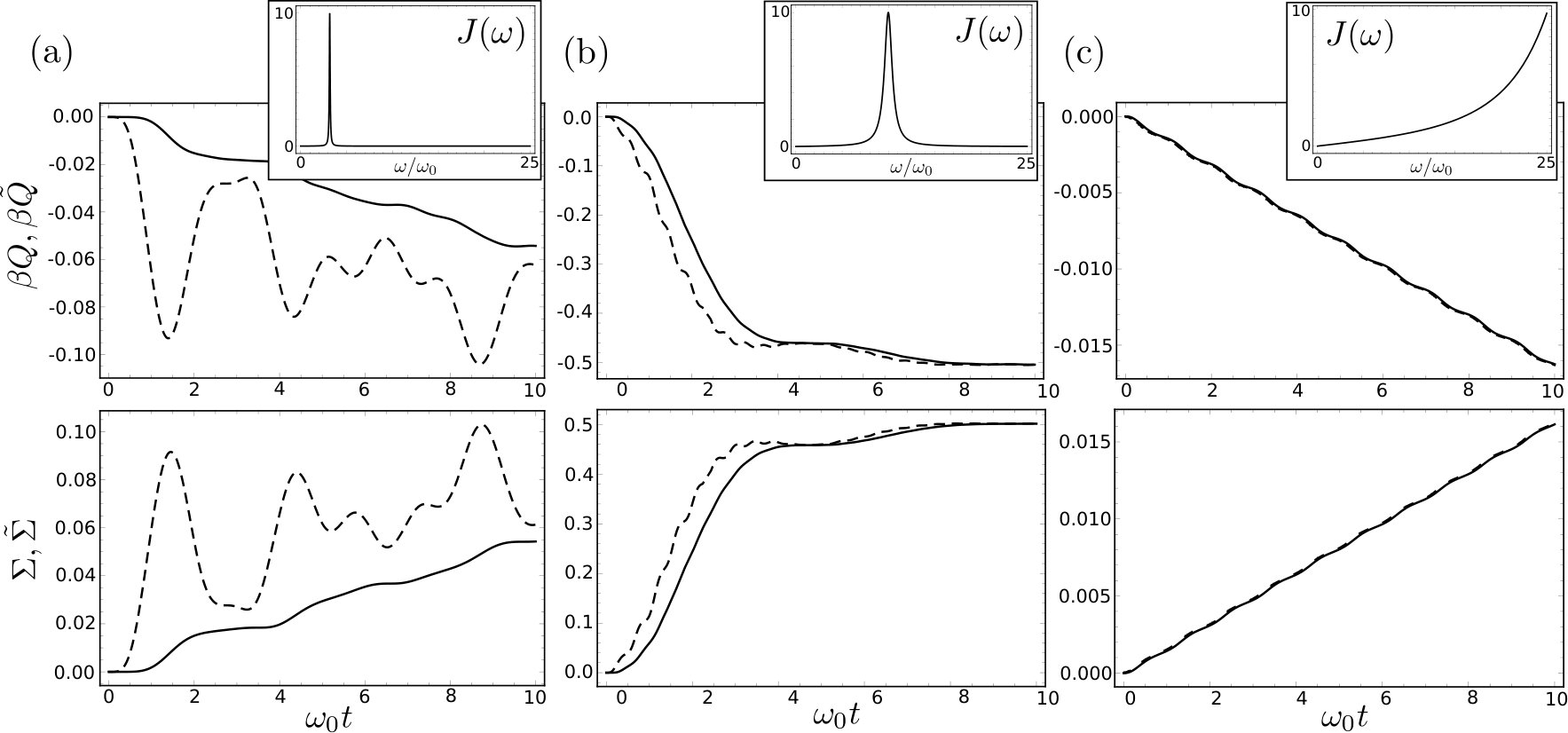 Figure 1
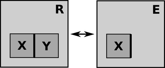 Figure 2
Peer Reviews
No public reviews on file for this paper yet. If you reviewed it on a platform where reviews are public (OpenReview, ICLR, NeurIPS, ICML), you can paste yours below so the community can read it here.
Videos
No videos yet. Explain this paper in a talk, walkthrough, or lecture? Add one.
Stochastic thermodynamics in the strong coupling regime:
An unambiguous approach based on coarse-graining
Philipp Strasberg
Massimiliano Esposito
Complex Systems and Statistical Mechanics, Physics and Materials Science, University of Luxembourg, L-1511 Luxembourg, Luxembourg
Abstract
We consider a classical and possibly driven composite system weakly coupled to a Markovian thermal reservoir so that an unambiguous stochastic thermodynamics ensues for . This setup can be equivalently seen as a system strongly coupled to a non-Markovian reservoir . We demonstrate that only in the limit where the dynamics of is much faster than , our unambiguous expressions for thermodynamic quantities such as heat, entropy or internal energy, are equivalent to the strong coupling expressions recently obtained in the literature using the Hamiltonian of mean force. By doing so, we also significantly extend these results by formulating them at the level of instantaneous rates and by allowing for time-dependent couplings between and its environment. Away from the limit where evolves much faster than , previous approaches fail to reproduce the correct results from the original unambiguous formulation, as we illustrate numerically for an underdamped Brownian particle coupled strongly to a non-Markovian reservoir.
I Introduction
Establishing the laws of thermodynamics for a given setup is not only beneficial for practical purposes, but also provides an important consistency check for the validity of the model and provides much deeper insights into the structure of the problem. Yet, establishing these laws for small-scale systems away from the well-established weak-coupling and Markovian limit can be very challenging.
This paper focuses on the case of a small, driven classical system in strong contact with a single environment. This case has attracted a lot of attention recently and was mostly tackled by introducing a Hamiltonian of mean force (HMF), classically Jarzynski (2004); Gelin and Thoss (2009); Seifert (2016); Talkner and Hänggi (2016); Philbin and Anders (2016); Jarzynski (2017); Miller and Anders (2017) as well as quantum-mechanically Gelin and Thoss (2009); Campisi et al. (2009a, b); Hilt et al. (2011); Pucci et al. (2013); Philbin and Anders (2016). However, the question of what exactly are the correct definitions for heat, internal energy and other quantities causes already controversies at the classical level Gelin and Thoss (2009); Seifert (2016); Talkner and Hänggi (2016); Jarzynski (2017).
We present an enlightening perspective on this problem by considering two coupled systems which are in weak contact with a large thermal reservoir and obey standard stochastic thermodynamics. By realizing that the system can be strongly coupled to the system , we see that the situation is equivalent to a system in strong contact with an environment . In fact, for many relevant scenarios it makes sense that the system only couples strongly to a subpart of the environment, but not to each degree of freedom of . This picture is also supported by our example at the end of the paper.
The benefit of our approach is that we start from a well-defined thermodynamics with unambiguous definitions and we can then compare under which conditions previous approaches based on the HMF coincide with them. Our framework can be seen as an applications of the laws of thermodynamics under coarse graining as detailed in Ref. Esposito (2012), also see Refs. Seifert (2011); Bo and Celani (2014).
*Outline: * We start by presenting the thermodynamic description of the combined system in contact with in Sec. II. We show what changes if we coarse-grain and consider the important limit where evolves much faster than such that it can be adiabatically eliminated and a closed thermodynamic description for alone emerges. In Sec. III we turn the situation around and start from a description of coupled to and derive an exact inequality. Based on this we recapitulate the thermodynamics previously established using the HMF and we show that we are able to rederive and greatly extend these results if evolves much faster than . Beyond that we explicitly quantify the difference in the two proposed definitions of entropy production and we use an example in Sec. IV to illustrate generic features in the thermodynamics of strongly coupled systems demonstrating that knowledge of the HMF alone does not suffice to reproduce the original thermodynamics. It also provides a strategy to identify a system if the initial setup is described at the level of . Sec. V summarizes the main implications of our findings.
II Setup
II.1 Basic quantities
A sketch of the setup is shown in Fig. 1. Two systems and interact with each other and their joint Hamiltonian is assumed to be of the form
[TABLE]
Here, the energy of system as well as the interaction energy can be time-dependent due to some externally controlled parameters . The energy of system is assumed to be time-independent.
Since the joint system is weakly coupled to a large thermal reservoir at inverse temperature , we assume that its dynamics can be modeled by a Markovian master equation (ME) of the form
[TABLE]
Here, denotes the probability to find the system in state at time . The rate matrix obeys which ensures conservation of probability []. Furthermore, we assume local detailed balance
[TABLE]
which allows a physical interpretation of the ME and especially a consistent thermodynamic description. The rest in this section then follows standard stochastic thermodynamics Schnakenberg (1976); Seifert (2012); Van den Broeck and Esposito (2015).
For this purpose we introduce the following quantities:
[TABLE]
Here, we have denoted the ensemble average with respect to any solution of the ME above by . Furthermore, the thermodynamic entropy coincides in the weak coupling regime with the definition of Shannon entropy.
Based on the definitions above, it is straightforward to derive the first law:
[TABLE]
(we define heat and work positive if they increase the energy of ). Furthermore, the second law states that the overall entropy production rate is postive:
[TABLE]
Its positity can be proven by noting the identity
[TABLE]
and using . Another useful identity is
[TABLE]
where the partial derivative indicates that the change of is evaluated at fixed . Here, we introduced the equilibrium (Gibbs, thermal) state
[TABLE]
which depends parametrically on time and denotes the equilibrium partition function. Also the concept of relative entropy,
[TABLE]
which is always positive for any two probability distributions and , will be used later on.
Finally, let us introduce the concept of a non-equilibrium free energy , which is defined for any state . Using this, we can reformulate the second law as
[TABLE]
Whenever a system (where could stand for depending on the situation) is at equilibrium, it is useful to note the relations
[TABLE]
for the equilibrium free energy, internal energy and entropy. Note that we use calligraphic letters to denote thermodynamic quantities at equilibrium.
Below, to keep a compact notation, we will often omit the dependence on in the notation.
II.2 Coarse-graining
We now shift our attention to system alone and mostly follow Ref. Esposito (2012) for the rest of this section. For this purpose we split the joint probability into a conditional and marginal probability as
[TABLE]
with and . It is not hard to deduce that evolves according to the ME
[TABLE]
where the new effective rate matrix is given by
[TABLE]
In general, it depends explicitly on time due to the time-dependence of and solving (19) is equally hard as solving the original ME unless further assumptions are made.
Nevertheless, there is an apparent second law related to the reduced dynamics of Esposito (2012):
[TABLE]
which can be rewritten as
[TABLE]
Here, we introduced the apparent heat flow
[TABLE]
and denotes the conditional Shannon entropy
[TABLE]
which fulfills with . Unfortunately, at this general level there is no relation between and the real heat flow making it hard to establish a local version of the first law. Furthermore, note that always underestimates the true entropy production .
II.3 Time-scale separation
There is an important limit, in which evolves much faster than and can be adiabatically eliminated. We will refer to this as time-scale separation (TSS). Within TSS one assumes that
[TABLE]
for . To get a simple description we also assume that for each given all states are connected, i.e., for all .
Under these conditions one can show that the conditional probabilities equilibrate and can be written as111Of course, there are also alternative parametrizations possible. For instance, with . This does not affect the resulting thermodynamics at the end.
[TABLE]
Normalization is ensured by choosing
[TABLE]
where denotes the ensemble average with respect to . Note that depends parametrically on time. In contrast, the equilibrium free energy has no time-dependence. Although it appears in the definition of , we remark that the reduced state of is not given by the equilibrium state .
Within TSS we denote the rate matrix by , which now depends only parametrically on time and greatly simplifies the solution of Eq. (19). Furthermore, it fulfills an effective local detailed balance relation of the form
[TABLE]
which makes the meaning of as a free energy landscape for system transparent. Using this, we can express the apparent heat flow (23) as
[TABLE]
which now coincides with the real heat flow:
[TABLE]
To prove Eq. (30) it is useful to note that
[TABLE]
where we used (26). Then, after realizing that and , we get
[TABLE]
Plugging this result into Eq. (29), we finally obtain
[TABLE]
which equals our original definition (6) within TSS.
Furthermore, it makes sense to rewrite the internal energy as where we introduced the average internal energy conditioned on the state :
[TABLE]
Formally, the first law remains the same as before
[TABLE]
In contrast to the general case, however, the time-dependence of all quantities comes only from the dynamical time-dependence of the system alone and the parametric dependence on . The same observation holds true for the second law of thermodynamics which can be expressed as
[TABLE]
Thus, within TSS we have indeed . For later purposes it will be also convenient to note the following two identities
[TABLE]
which look remarkably similar to Eqs. (16) and (17). Proving them follows from straightforward though tidious algebraic manipulations, which we will not display here.
Finally, we briefly mention how to extend the results above to the stochastic level following the well-established procedure Seifert (2012); Van den Broeck and Esposito (2015). This will also underline the fact that any information about enters only statically in the description. If the system starts at time in state , jumps at time to and stays in that state until it jumps at time to , etc., we denote this trajectory by . Then, the fluctuating internal energy at each instant is given by
[TABLE]
The work along the trajectory becomes
[TABLE]
and the stochastic entropy is defined as
[TABLE]
Finally, the heat can be decomposed as
[TABLE]
where the sum indexed by runs over all jumps which have happened from to . Since obeys a Markovian ME with rates that fulfill the local detailed balance relation (28), it is clear that the integral and detailed fluctuation theorems are also obeyed, e.g.,
[TABLE]
where and denotes an ensemble average over all trajectries .
III The Hamiltonian of mean force
III.1 Exact identities
In this section we turn the situation around and consider a system in contact with an environment as shown on the right hand side of Fig. 1 and we only use in Sec. III.2 the decomposition . We assume that the combined system is isolated and obeys an Hamiltonian dynamics with an Hamiltonian
[TABLE]
where denotes a microstate of the environment. Note that we will in general denote thermodynamic quantities in this section by a “tilde” to distinguish them from previously introduced quantities. Their relation will be clarified in Sec. III.2.
As in Ref. Seifert (2016); Talkner and Hänggi (2016), we assume that the initial state of reads
[TABLE]
where is an arbitrary initial system state and denotes the equilibrium state of conditioned on a microstate of the system. Clearly, is defined as in Eq. (27) with replaced by . The state can be more elegantly expressed by introducing the HMF,
[TABLE]
which has been successfully used for a long time in thermostatics Kirkwood (1935); Roux and Simonson (1999). Using this, we find
[TABLE]
and also the important relation
[TABLE]
Given the initial state (45), we follow Ref. Esposito et al. (2010) and define an entropy production
[TABLE]
which measures the deviation of the true state from an idealized reference state . Note that definition (49) differs from Ref. Esposito et al. (2010) only in the choice of the reference state We discuss in Appendix A how both are related. We will now show that Eq. (49) coincides with the definition used in Ref. Seifert (2016) as was independently and simultaneously noted in Ref. Miller and Anders (2017).
It is convenient to rewrite Eq. (49) as
[TABLE]
where we used that the Shannon entropy of the global system remains constant under Hamiltonian dynamics, . Furthermore, we use the notation for any time-dependent function . Now, in accordance with phenomenological nonequilibrium thermodynamics, we would like to split into two parts:
[TABLE]
Without additional information, there is obviously no unique splitting of these two quantities at this formal level, which essentially translates the results of Ref. Talkner and Hänggi (2016) into our framework. For the moment we will use the following definitions, which comply with the suggestions of Ref. Seifert (2016):
[TABLE]
The latter can be also rewritten as
[TABLE]
if we use the generally accepted definition for work . Assuming the first law of thermodynamics to be valid in the strong coupling case, this then implies a definition for internal energy:
[TABLE]
Introducing the non-equilibrium free energy
[TABLE]
we can alternatively write Eq. (51) as
[TABLE]
The definitions above of , , , and seem to provide a satisfactory extension of thermodynamics to the strong-coupling case and they coincide with the definitions used by Seifert, who further motivates them by arguments of equilibrium statistical mechanics Seifert (2016). In addition to Ref. Seifert (2016), we have seen that the framework can be even extended by allowing for a time-dependence in the coupling , too.
Nevertheless, the approach above should be taken with care because it is ambiguous Talkner and Hänggi (2016), and is not formulated at the level of instantaneous rates implying that the positivity of entropy production (51) crucially relies on the choice of initial state (45).
III.2 Reduced thermodynamics description in
We now clarify this situation by returning to our previous results in Sec II.3. where we assumed that the environment is made of two parts, . The first part is strongly coupled to the system and is explicitly described. The second part is an ideal weakly coupled and Markovian thermal reservoir. Under these assumptions the ME (2) and the full Hamiltonian dynamics give rise to the same description in the reduced space . This implies, e.g., that the work computed within the ME framework [see Eq. (5)] coincides with the work computed using the exact Hamiltonian dynamics as in Sec. III.1.
In the limit of TSS, instantaneously equilibrates with respect to a given microstate of . Thus, the initial requirement (45) is not only fulfilled initially but at any time . This implicitly means that for any fixed value of , the global equilibrium steady state reads
[TABLE]
where is the bare Hamiltonian of . As a result, the HMF introduced in Eq. (46) coincides with
[TABLE]
which can be regarded as the HMF of only. Using the last equation together with (37) and (38), it is not hard to deduce the following two relations:
[TABLE]
Thus, apart from a time-independent additive constant the definitions for internal energy and system entropy within TSS coincide with the definitions based on the HMF. Furthermore, since both approaches agree on the definition of work, we can show for the heat flow that
[TABLE]
Thus, within TSS we agree on this definition too and are able to derive the first law at the level of instantaneous rates. Likewise, we can also prove the positivity of the entropy production rate by noting that
[TABLE]
As a preliminary summary we have thus shown that within TSS, the framework introduced in Ref. Seifert (2016) is thermodynamically consistent and can be greatly extended. Furthermore, no ambiguity is left within our approach which allows us to refute the criticism raised in Ref. Talkner and Hänggi (2016) for our setup.
It is interesting to ask what happens away from TSS when does not instantaneously conditionally equilibrate and is thus dynamically evolving. It is then possible to show that the framework of Sec. III.1 does not coincide with the original thermodynamic description of Sec. II anymore. For instance, we prove in Appendix B that the difference in entropy production can be expressed as
[TABLE]
Thus, overestimates by the relative entropy between the true state of and an idealized state of the form (45). Also, the rate of change of can be negative. This and other features are explicitly demonstrated in the next section with the help of an example where the ME description in exactly coincides with the reduced Hamiltonian dynamics.
To conclude, when it is possible to separate out the strongly coupled and non-Markovian degrees of freedom from the environment , then the following hierarchy of inequalities holds,
[TABLE]
The equality holds in the limit of TSS. Each of the entropy production in Eq. (65) corresponds to a different layer of the description. assumes to be conditionally (versus ) equilibrated and, of course, implicitly to be equilibrated. assumes only an ideal reservoir and is an exact result which can be applied to any Hamiltonian dynamics (44) as long as the initial condition is of the form (45).
IV Discrepancy in the non-Markovian regime
Within TSS, i.e., whenever the environment behaves Markovian by instantaneously adapting to the microstate of the system , we have proven the equivalence of the coarse-grained thermodynamic framework from Sec. II.3 with the approach based on the HMF. In principle, both frameworks can be also applied beyond TSS and we will now provide a counterexample showing that the HMF-approach then no longer coincides with the standard framework of Sec. II.
We consider the example of driven Brownian motion thereby demonstrating that our main results above do not only hold for dynamics on discrete states but also for continuous variables. The global Hamiltonian with mass-weighted coordinates is specified by Weiss (2008); Sekimoto (2010)
[TABLE]
and we identify in the following and use . We relaxed the notation meaning with the energy associated to the microstate and a microstate of the bath is given by specifying for all . Furthermore, the spectral density (SD) of the bath is defined as and parametrized by
[TABLE]
Here, controls the overall coupling strength between the system and the environment and changes the shape of the SD from a pronounced peak around for small to a rather unstructured and flat SD for large .
The corresponding Langevin equation for this setup reads Weiss (2008); Sekimoto (2010)
[TABLE]
with the friction kernel
[TABLE]
and the noise , which obeys the statistics
[TABLE]
We see that for an Ohmic SD (times a high-frequency cutoff as usual) we obtain and this gives the standard Langevin equation with Gaussian white noise. Unfortunately, our SD (69) is not Ohmic unless we scale , and send . This implies an Ohmic SD for sufficiently large :
[TABLE]
Establishing a consistent thermodynamic framework for the general Langevin Eq. (70) cannot be done using standard tools from stochastic thermodynamics. One route, however, could be to take the definitions from Sec. III and to apply them here. Application of these definitions is facilitated by the fact that for a Brownian motion Hamiltonian the HMF coincides with the bare system Hamiltonian, i.e., , which can be directly checked by evaluating the Gaussian integrals. Thus, the change in internal energy and system entropy read and . That is to say, the HMF-approach uses for this examples the standard weak-coupling definitions irrespective of the spectral properties of the bath. Furthermore, since work can be computed using , we obtain and , too. However, to access the dynamics of the system, we would have to simulate the non-Markovian Langevin equation (70), which is numerically demanding.
We therefore follow a different strategy and identify a subsystem , which transforms the non-Markovian system to a Markovian system . This is most conveniently done by identifying a collective degree of freedom in the environment defined via
[TABLE]
In this context, is also known as a reaction coordinate. It has been shown to successfully model the dynamics of non-Markovian open quantum systems (see, e.g., Refs. Prior et al. (2010); Martinazzo et al. (2011); Woods et al. (2014); Iles-Smith et al. (2014)) and has been recently proposed as a method to establish a consistent thermodynamic framework beyond the Markovian and weak-coupling approximation Strasberg et al. (2016); Newman et al. (2017).
We skip the details of the derivation, which can be looked up in the literature Prior et al. (2010); Martinazzo et al. (2011); Woods et al. (2014); Iles-Smith et al. (2014); Strasberg et al. (2016); Newman et al. (2017), and only state the main result. After the transformation, the Hamiltonian becomes
[TABLE]
where the new SD of the “residual environment” is defined and for the choice (69) given by
[TABLE]
This SD immediately yields the coupled set of Markovian Langevin equations
[TABLE]
with Gaussian white noise .
Following standard procedures Sekimoto (2010), we can associate a Fokker-Planck equation for the probability distribution to the set of Langevin equations above. It reads
[TABLE]
where we defined , and introduced the matrices
[TABLE]
and whose only non-zero component is . We emphasize that Eq. (80) describes the exact dynamics in . No approximation has been made in any of the steps above (apart from assuming an initially equilibrated reservoir state).
An advantage of this Fokker-Planck equation is that the dynamics of the first and second cumulants are closed. In fact, the equations of motion for the first cumulants (with ) couple only to themselves and the same is true for the second cumulants . Thus, an initially Gaussian state will stay Gaussian for all times. Computing the time-evolution of the first two cumulants based on an initial condition of the form (45) can then be easily done numerically. Because standard stochastic thermodynamics applies to Eqs. (79) or (80), we have direct access to averaged thermodynamic quantities for introduced in Sec. II, also see Ref. Sekimoto (2010). Furthermore, because we have the exact dynamics in , we also get the exact reduced dynamics of by tracing over , consequently giving direct access to the time evolution of and . Thus, our Markovian embedding strategy has allowed us to circumvent the difficulty to simulate the non-Markovian Langevin equation (70).
Results of the simulation are shown in Fig. 2. We vary the SD from a strongly non-Markovian situation (shown on the left) to a Markovian but strong-coupling situation (on the right) by changing and . For each we compare the integrated heat flows and (upper panel) and the integrated entropy production and (lower panel). The following main features are observable: for large the assumption of TSS is justified and quantities defined in Sec. II.3 and III agree perfectly. In fact, is directly linked to the rate of relaxation of the reaction coordinate , but does not directly couple to the system degrees of freedom . Thus, a large corresponds to the limit of TSS as introduced in Eq. (25). Away from that limit, however, we observe that differs significantly from and the same observation is true for the different definitions of entropy production, too. Also, although Eq. (51) is always obeyed, the rate of can become negative. Furthermore, we can also confirm the validity of Eq. (64), .
V Summary
We clarified important questions in the framework of strong-coupling thermodynamics. Our main achievements are the following:
1) Justification of the HMF within TSS. Within the limit of TSS, the framework provided in Ref. Seifert (2016) is thermodynamically consistent for arbitrary system states and the HMF is a legitimate tool to investigate the thermodynamics of systems in strong contact with a single environment.
*2) No ambiguity. * Any ambiguity is removed in our framework and the concerns put forward in Ref. Talkner and Hänggi (2016) do not apply. The reason for this is that we start from a well-defined weak coupling framework. Especially and contrary to previous attempts, we do not use the first law to define heat, but have an alternative and unambiguous definition for it.
*3) Extension of previous results. * Thanks to the TSS, we were able to significantly extend previous results by formulating them at the level of instantaneous rates instead of integrated quantities and by allowing also for a time-dependence in the system-environment coupling.
*4) Difficulties in the non-Markovian regime. * Away from TSS, the framework of Ref. Seifert (2016) does not match the original thermodynamic picture though Eq. (49) is always obeyed. Thus, we observe that in order to establish the original laws of thermodynamics in the non-Markovian regime (where the environment is also dynamically evolving), one is forced to fully take into account the (thermo)dynamics of and . Any effective description at this stage will in general miss important pieces in the first or second law. This complies with the point of view put forward in Ref. Strasberg et al. (2016); Newman et al. (2017).
Recently, two alternative approaches were put forward in Ref. Jarzynski (2017) by starting from the isothermal-isobaric ensemble and by taking pressure and volume effects into account. These approaches correctly reproduce the macroscopic limit by introducing the notion of “thermodynamic volume” for a microscopic system. The “bare representation” in Ref. Jarzynski (2017) shows that it is possible to retain the original weak coupling definitions of internal energy and entropy by shifting our attention to enthalphy and Gibbs free energy instead. If the isobaric -contribution is absent or blindly ignored, then the “partial molar representation” in Ref. Jarzynski (2017) coincides with the approach in Sec. III.222To compare notation, we have without -terms that the Gibbs free energies in Ref. Jarzynski (2017) are related to our free energies via , and the solvation Hamiltonian of mean force becomes . However, note that the -term in Ref. Jarzynski (2017) is actually only negligible at weak coupling. Then, and all the different frameworks coincide with the weak coupling limit. These alternative approaches should be therefore also derivable within TSS, but we expect that outside the limit of TSS they will mismatch again.
Finally, we would like to mention that the framework of Sec. III can be used in principle also beyond TSS, for instance, if it is impossible to find a splitting or if the dynamical simulation of the environment becomes unfeasible. It then nevertheless has to be treated with care and further consistency checks still need to be carried out such as, for instance, the implication of the correct thermodynamic laws in the limit of reversible transformations as investigated in Ref. Esposito et al. (2015).
*Acknowledgements. * Financial support by the National Research Fund Luxembourg (project FNR/A11/02) and by the European Research Council (project 681456) is acknowledged.
Appendix A Relation between the entropy production in Eq. (49) and Ref. Esposito et al. (2010)
In Ref. Esposito et al. (2010), the entropy production of an Hamiltonian dynamics (44) with an initial condition of the form was defined as
[TABLE]
This result is very close in spirit to the entropy production (49) that we derived in this paper for the same Hamiltonian dynamics but with an initial condition of the form (45). It measures the deviation of the true state from an idealized product state where the environment is always at equilibrium instead of conditionally at equilibrium.
The only meaningful comparison between the two expressions requires to consider situations where the two classes of initial conditions coincide, namely when and the interaction is only turned on afterwards. In this case, we find that
[TABLE]
This relation can be rewritten as a difference between the non-equilibrium free energy (56) and the non-equilibrium free energy corresponding to the scheme of Ref. Esposito et al. (2010)
[TABLE]
Explicitly,
[TABLE]
In general, there is no bound for this difference.
Appendix B Proof of Eq. (64)
From Eq. (14) we deduce that . Thus, with Eq. (57) we immediately get the first line of Eq. (64),
[TABLE]
To prove the second, we look at and in detail. Since the formalism using the HMF in Sec. III assumes that the environment starts in a conditionally equilibrated state , Eqs. (60) and (61) are valid at . Straightforward algebra then gives
[TABLE]
At later times, using the definitions (52) and (55), we find that
[TABLE]
Next, from Eq. (59) together with (26) we obtain
[TABLE]
Thus, we have explicitly
[TABLE]
and consequently,
[TABLE]
which proves the second line of Eq. (64).
The reference list from the paper itself. Each links out to its DOI / PubMed record.
- 1Jarzynski (2004) C. Jarzynski, “Nonequilibrium work theorem for a system strongly coupled to a thermal environment,” J. Stat. Mech. P 09005 (2004).
- 2Gelin and Thoss (2009) M. F. Gelin and M. Thoss, “Thermodynamics of a subensemble of a canonical ensemble,” Phys. Rev. E 79 , 051121 (2009) . · doi ↗
- 3Seifert (2016) U. Seifert, “First and second law of thermodynamics at strong coupling,” Phys. Rev. Lett. 116 , 020601 (2016).
- 4Talkner and Hänggi (2016) P. Talkner and P. Hänggi, “Open system trajectories specify fluctuating work but not heat,” Phys. Rev. E 94 , 022143 (2016).
- 5Philbin and Anders (2016) T. G. Philbin and J. Anders, “Thermal energies of classical and quantum damped oscillators coupled to reservoirs,” J. Phys. A: Math. Theor. 49 , 215303 (2016).
- 6Jarzynski (2017) C. Jarzynski, “Stochastic and macroscopic thermodynamics of strongly coupled systems,” Phys. Rev. X 7 , 011008 (2017) . · doi ↗
- 7Miller and Anders (2017) H. J. D. Miller and J. Anders, “Entropy production and time-asymmetry in the presence of strong interactions,” ar Xiv: 1703.03764 (2017).
- 8Campisi et al. (2009 a) M. Campisi, P. Talkner, and P. Hänggi, “Fluctuation theorem for arbitrary open quantum systems,” Phys. Rev. Lett. 102 , 210401 (2009 a).