Multi-parameter One-Sided Monitoring Test
Guangyu Zhu, Jiahua Chen

TL;DR
This paper introduces a new, more powerful statistical test for monitoring multiple quality indices in forestry products, improving upon traditional likelihood ratio tests by balancing size control and power.
Contribution
A novel testing method that slightly relaxes size control to achieve significantly higher power in multi-parameter one-sided hypothesis testing.
Findings
New test maintains good size control
Significantly more powerful than likelihood ratio test
Performs well in monitoring multiple quality indices
Abstract
Multi-parameter one-sided hypothesis test problems arise naturally in many applications. We are particularly interested in effective tests for monitoring multiple quality indices in forestry products. Our search reveals that there are many effective statistical methods in the literature for normal data, and that they can easily be adapted for non-normal data. We find that the beautiful likelihood ratio test is unsatisfactory, because in order to control the size, it must cope with the least favorable distributions at the cost of power. In this paper, we find a novel way to slightly ease the size control, obtaining a much more powerful test. Simulation confirms that the new test retains good control of the type I error and is markedly more powerful than the likelihood ratio test as well as many competitors based on normal data. The new method performs well in the context of monitoring…
Click any figure to enlarge with its caption.
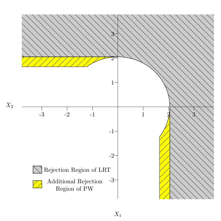 Figure 1
| 0.5 | ||||||
|---|---|---|---|---|---|---|
| 5.64 | 5.37 | 4.98 | 4.58 | 4.12 | 3.47 |
| LRT | PW | mLR | LRT | PW | mLR | LRT | PW | mLR | LRT | PW | mLR | LRT | PW | mLR | |
|---|---|---|---|---|---|---|---|---|---|---|---|---|---|---|---|
| (0,0) | 4.49 | 5.46 | 5.08 | 3.79 | 4.79 | 5.05 | 3.05 | 4.03 | 4.98 | 2.46 | 3.43 | 5.00 | 1.66 | 2.64 | 4.94 |
| (0,-.1) | 1.34 | 4.23 | 1.56 | 1.54 | 3.03 | 2.12 | 1.62 | 2.91 | 2.69 | 1.34 | 2.70 | 2.87 | 1.18 | 3.62 | 3.65 |
| (0,-.2) | 1.23 | 5.13 | 1.40 | 1.11 | 3.60 | 1.56 | 1.20 | 3.32 | 2.04 | 1.20 | 3.69 | 2.59 | 1.15 | 4.90 | 3.55 |
| (0,-.3) | 1.14 | 5.12 | 1.31 | 1.14 | 4.48 | 1.58 | 1.21 | 4.28 | 2.05 | 1.18 | 4.50 | 2.55 | 1.13 | 4.89 | 3.45 |
| (.1,.1) | 84.4 | 84.4 | 85.7 | 27.6 | 27.9 | 32.4 | 16.1 | 17.1 | 22.3 | 11.2 | 12.9 | 18.8 | 7.74 | 10.2 | 17.3 |
| (.2,.2) | 100 | 100 | 100 | 75.8 | 75.8 | 80.1 | 46.8 | 47.3 | 56.3 | 32.4 | 34.1 | 45.3 | 23.6 | 27.5 | 40.8 |
| (.3,.3) | 100 | 100 | 100 | 97.9 | 97.9 | 98.6 | 80.3 | 80.4 | 86.2 | 62.2 | 63.1 | 74.3 | 49.4 | 53.4 | 68.7 |
| (.4,.4) | 100 | 100 | 100 | 99.9 | 99.9 | 99.9 | 96.3 | 96.3 | 97.9 | 86.2 | 86.5 | 92.5 | 75.1 | 77.6 | 88.3 |
| (0,.1) | 33.9 | 34.1 | 36.0 | 12.4 | 13.4 | 15.5 | 8.88 | 10.6 | 13.0 | 6.79 | 9.64 | 12.4 | 5.72 | 12.6 | 13.5 |
| (0,.2) | 86.1 | 86.1 | 87.3 | 33.4 | 34.3 | 38.8 | 23.1 | 26.3 | 30.4 | 19.4 | 27.5 | 29.6 | 18.4 | 38.9 | 33.9 |
| (0,.3) | 99.5 | 99.5 | 99.6 | 62.7 | 63.1 | 68.0 | 46.7 | 50.8 | 55.9 | 42.3 | 56.0 | 55.6 | 41.9 | 67.2 | 61.3 |
| (0,.4) | 100 | 100 | 100 | 86.4 | 86.6 | 89.3 | 72.0 | 75.3 | 79.2 | 68.8 | 82.0 | 79.7 | 68.2 | 87.3 | 83.6 |
| (-.1,.1) | 8.19 | 10.3 | 9.04 | 7.07 | 9.89 | 9.14 | 6.26 | 10.1 | 9.44 | 5.83 | 11.7 | 10.6 | 5.53 | 16.7 | 13.4 |
| (-.2,.2) | 21.1 | 25.9 | 22.7 | 19.6 | 27.8 | 23.6 | 18.7 | 31.4 | 25.2 | 18.4 | 37.5 | 28.4 | 18.6 | 40.5 | 34.4 |
| (-.3,.3) | 44.0 | 51.2 | 46.1 | 42.1 | 55.9 | 47.5 | 41.8 | 62.8 | 50.9 | 41.7 | 66.8 | 54.8 | 41.6 | 67.1 | 61.3 |
| (-.4,.4) | 69.3 | 76.2 | 71.2 | 68.5 | 81.8 | 73.2 | 68.3 | 86.2 | 75.9 | 68.3 | 87.4 | 79.3 | 68.5 | 87.4 | 83.7 |
| Setting I | Setting II | Setting III | |||||||
|---|---|---|---|---|---|---|---|---|---|
| LRT | PW | mLR | LRT | PW | mLR | LRT | PW | mLR | |
| 2.93 | 3.86 | 5.91 | 4.50 | 5.20 | 8.20 | 6.29 | 9.34 | 12.08 | |
| 47.35 | 52.55 | 62.01 | 7.20 | 10.30 | 13.30 | 16.45 | 25.55 | 25.87 | |
| 95.81 | 96.83 | 98.20 | 14.30 | 22.20 | 24.70 | 29.18 | 44.44 | 42.93 | |
| Setting I | Setting II | Setting III | |||||||
|---|---|---|---|---|---|---|---|---|---|
| LRT | PW | mLR | LRT | PW | mLR | LRT | PW | mLR | |
| 2.79 | 3.76 | 5.69 | 76.07 | 77.48 | 86.23 | 99.99 | 99.99 | 100.0 | |
| 4.17 | 5.43 | 7.96 | 6.25 | 8.96 | 12.30 | 13.80 | 21.82 | 23.51 | |
| 6.01 | 8.72 | 11.27 | 14.21 | 21.17 | 22.84 | 32.87 | 47.61 | 45.44 | |
| 5% | 50% | |
|---|---|---|
| In-Grade | 2.64 | 5.28 |
| 2011/2012 | 1.87 | 3.71 |
Peer Reviews
No public reviews on file for this paper yet. If you reviewed it on a platform where reviews are public (OpenReview, ICLR, NeurIPS, ICML), you can paste yours below so the community can read it here.
Videos
No videos yet. Explain this paper in a talk, walkthrough, or lecture? Add one.
Taxonomy
TopicsAdvanced Statistical Methods and Models · Statistical Methods and Applications · Spectroscopy and Chemometric Analyses
Multi-parameter One-Sided Monitoring Test
Guangyu Zhu
Department of Statistics, University of British Columbia, Canada
Jiahua Chen
Research Institute of Big Data, University of Yunnan, China
Department of Statistics, University of British Columbia, Canada
The authors gratefully acknowledge funding from NSERC Grant RGPIN-2014-03743, a Collaborative Research and Development Grant from NSERC and FPInnovations, and the “a thousand talents” program through Yunnan University. We are also indebted to the Forest Products Stochastic Modelling Group centered at the University of British Columbia (UBC): members of this group from FPInnovations in Vancouver, Simon Fraser University, and UBC provided stimulating discussions of the long-term monitoring program to which this paper contributes.
Abstract
Multi-parameter one-sided hypothesis test problems arise naturally in many applications. We are particularly interested in effective tests for monitoring multiple quality indices in forestry products. Our search reveals that there are many effective statistical methods in the literature for normal data, and that they can easily be adapted for non-normal data. We find that the beautiful likelihood ratio test is unsatisfactory, because in order to control the size, it must cope with the least favorable distributions at the cost of power. In this paper, we find a novel way to slightly ease the size control, obtaining a much more powerful test. Simulation confirms that the new test retains good control of the type I error and is markedly more powerful than the likelihood ratio test as well as many competitors based on normal data. The new method performs well in the context of monitoring multiple quality indices.
Keywords: Bootstrap; Composite likelihood; Density ratio model; Empirical likelihood; Multiple sample; Random effect.
1 Introduction
The research problem in this paper is motivated by an application. The reliability of a wood structure heavily depends on the mechanical strength of its component wood. It is important to closely monitor the dynamic wood strength distribution of solid lumber over time. This is done through data collected via a random sample from the target populations and the subsequent data analysis. A few weak components have potentially severe consequences for the structure, so the lower quantiles of the strength distribution have received the most attention. See the lumber-quality monitoring procedures specified in the American Society for Testing and Materials (ASTM) Standard D1990 (ASTM, 1991). This is also evident from the recent report by Verrill et al. (2015), which examined the performance of various tests in the context of 5% quantiles.
Clearly, even if the strength distribution of the wood product meets the quality standard for the lower quantiles, the median or mean strengths could be significantly lower than the norm. The reliability of the structure could still be seriously compromised. This suggests the need to develop a monitoring test procedure for several quality indices simultaneously. We aim to draw the attention of practitioners to this need and to develop an effective and easy-to-use test procedure.
The application easily translates into a statistical question. We wish to statistically detect potential danger arising when the values of several user-selected parameters fall below well-established standards. In other words, we seek a test for multi-parameter one-sided null and alternative hypotheses. More abstractly, suppose we have a sample from distribution , and is a vector-valued parameter or functional of . We wish to test the hypothesis
[TABLE]
for a specific known vector \mbox{\boldmath\theta}^{*}, where the inequality is interpreted to be component-wise. Because of the invariance property, without loss of generality, we may take \mbox{\boldmath\theta}^{*}={\bf 0}; this will be assumed hereafter unless otherwise indicated. The dimension of will be denoted as . Clearly, many existing tests can easily be adapted to this problem. However, we suggest that none of them seem to exactly fit, and additional research is needed.
Under the normal model, the likelihood ratio test (LRT) provides standard solutions to the current pair of opposing hypotheses and and similarly formulated pairs of opposing hypotheses. Statisticians must determine the appropriate rejection region to ensure that the LRT has the size specified by the user. Along this line, Robertson & Robertson (1988) worked out the solution to the LRT problem for the case where is known to be I. Perlman (1969) solved the LRT problem where is unknown.
By the standard definition in mathematical statistics, the size of a test is the supremum of its type I error. When the null hypothesis is composite, i.e., it contains many distributions, the size of the test is the type I error in the worst scenario, or at the least favorable null distribution. Controlling the size of the test can therefore lead to a pessimistic procedure: the type I error under the likely true data-generating distribution is far below the size of the test that leads to compromised power. This is particularly true for the LRT for multi-parameter one-sided hypotheses. Perlman & Wu (2003) and Perlman & Wu (2006) examined the rejection region of the LRT in many situations and developed more powerful tests accordingly. Such research is often motivated by medical studies, where the aim is often to assess whether a therapy has a beneficial effect on multiple outcomes simultaneously relative to a control. The specifics of these one-sided hypotheses vary depending on the medical problem. For instance, O’Brien (1984) and Tang et al. (1989) proposed and extended a generalized least-squares test that is most powerful when the true population mean is near a specific line in the alternative space. In clinical studies with multiple outcomes, researchers may wish to confirm that a new treatment is superior in at least one of the outcomes and equivalent on the rest of the outcomes, in comparison with the control. Tamhane & Logan (2004) targeted this problem with a test derived from the union–intersection test of (Roy, 1953) and the intersection–union test of (Berger, 1982). We refer to Wassmer et al. (1999) for a more detailed review of this area and Lachin (2014) for recent advances.
The hypothesis of interest in this paper, (1), is similar to but different from those considered in the above papers. We investigate the direct application of the standard LRT to (1) and discover that a specific version of the LRT leads to a much improved procedure that is particularly useful for our application. We find a novel way to mildly relax the size control to obtain a much more powerful test. Simulation confirms that the new test retains tight control of the type I error and is markedly more powerful than the LRT as well as many of its competitors based on normal data. The new method performs well in the context of monitoring multiple quality indices.
The paper is organized as follows. In Section 2, we revisit some basics of the LRT, introduce the new test, and review existing methods for normal data and one-sided multi-parameter hypotheses. In Section 3, we give a brief background on the monitoring test for forestry products and the application of the proposed method. In Section 4, we present simulation results. We conclude in Section 5.
2 Proposed and related methods
The new approach was developed as a result of our observation of the LRT under the normal model. For this reason, we first quickly revisit the standard likelihood approach and then introduce our approach.
2.1 LRT statistic
Suppose we have an independent and identically distributed (iid) sample from a -dimensional multi-normal distribution \mbox{MVN}(\mbox{\boldmath\mu},\mbox{\boldmath\Sigma}). We first consider the test problem for
[TABLE]
Let X denote the sample mean and
[TABLE]
a slightly altered sample variance. It is well known that X and S together are complete and sufficient for and under the normal model. Hence, we may develop a likelihood-based method as if they are the only observations.
After some simple algebra, the log-likelihood function is found to be
[TABLE]
To develop an LRT, we search for the maximum point of \ell_{n}(\mbox{\boldmath\mu},\mbox{\boldmath\Sigma}) under the null hypothesis and under the full model. The solution under the full model is well known, with the unconstrained maximum likelihood estimators of and given by
[TABLE]
This implies
[TABLE]
The solution under the null model is algebraically simple but slightly more abstract. For each fixed , we find
[TABLE]
This leads to the profile log-likelihood function of :
[TABLE]
The second equality is obtained by a linear algebra result for any vector and , and by
[TABLE]
Clearly, the profile likelihood is maximized if and only if (\mbox{\bf X}-\mbox{\boldmath\mu})^{T}\mbox{\bf S}^{-1}(\mbox{\bf X}-\mbox{\boldmath\mu}) is minimized with respect to in the space of the null hypothesis. Let the solution to the minimization problem be \hat{\mbox{\boldmath\mu}}_{0}. Geometrically, it is the projection of X onto the null space in terms of the Mahalanobis distance defined through the covariance matrix S. Subsequently, we find the generic expression of the LRT statistic:
[TABLE]
Note that is monotonic in
[TABLE]
Thus, the rejection region of the LRT statistic has the generic form
[TABLE]
for some , which is called the critical value of the test.
By classical theory in mathematical statistics, if the size of the test is set to , then the critical value will be chosen so that
[TABLE]
where we use {\mbox{{Pr}}}(\cdot;\mbox{\boldmath\mu},\mbox{\boldmath\Sigma}) to indicate that the calculation is under the \mbox{MVN}(\mbox{\boldmath\mu},\mbox{\boldmath\Sigma}) distribution. According to Perlman (1969), the supremum is attained asymptotically when \mbox{\boldmath\mu}\to 0 and approaches some singular matrix. Specifically, he proved that for defined by (1),
[TABLE]
where denotes an F-distributed random variable with and degrees of freedom. In other words, an LRT of size will choose such that
[TABLE]
2.2 Proposed test
The choice of in the LRT in (8) ensures that the type I error is at most at any (\mbox{\boldmath\mu},\mbox{\boldmath\Sigma})\in H_{0}. When the dimension of the data , the type I error is maximized when \mbox{\boldmath\mu}=\bf{0} and where is the correlation coefficient. If the observations are from a distribution with \mbox{\boldmath\mu}={\bf 0} and , the type I error is far lower than . In many applications, the user may be confident that . If so, this choice is far too conservative. The size of the test over the region of interest is much lower than the designated . As a consequence, the power of the test is also much lower.
This consideration begs a question on the type I error of the test at \mbox{\boldmath\mu}=0 and a given . Interestingly, an answer is readily available from Nüesch (1966). To state this result, we first introduce some notation. When X is \mbox{MVN}(\mbox{\boldmath\mu},\mbox{\boldmath\Sigma}), we use the simplified notation
[TABLE]
Let be the collection of all nonempty subsets of . We use for the th entry of vector X. For any s\in\mbox{\mathcal{S}}, we use for the subvector of X consisting of components of such that . Let be the complement of . With these, we use \mbox{\boldmath\Sigma}_{s} for the covariance matrix of and \mbox{\boldmath\Sigma}_{s^{\prime}|s} for the covariance matrix of conditional on . We use the convention that when is empty {\mbox{{Pr}}}\{\mbox{\boldmath\Sigma}_{s^{\prime}|s}\}=1. We use for the size of . In the following theorem, is the LRT statistic defined earlier.
Theorem 1**.**
In the current setting, for any ,
[TABLE]
In other words, the distribution of is a finite mixture of -distributions. The proof of this theorem is technically involved; we refer to Nüesch (1966) for the details.
The probabilities in the above theorem have generic analytical expressions that can be found in Kendall (1941). We are particularly interested in the case . When , without loss of generality, we assume that has marginal variances and denote the correlation coefficient as . For such that , it is easy to see that
[TABLE]
When , the correlationship coefficient specified by \mbox{\boldmath\Sigma}^{-1} is . Let be two independent random variables. Then, and have correlation when in the range of 0 and . Hence,
[TABLE]
In other words, we have
[TABLE]
Consequently, if the value of is known and the observed value of is , we would have evaluated the value of the test to be
[TABLE]
This would lead to a much more powerful test than the classical LRT. For instance, we would reject when when is known to be [math], while the LRT does not reject in this case. See Table 1 for the critical values. The LRT uses the critical value at , corresponding to the least favorable distribution.
Motivated by the above discussion and calculations, we propose a new test for . First, we obtain the value of and the sample correlation coefficient . With the observed value , we compute
[TABLE]
The test rejects when , where is the designated size of the test.
Our idea is not limited to . The analytical form of (the p-value of the test) is more complex in the general case but can be calculated according to Theorem 1. We do not present the details here since the interested user can work them out with some algebraic effort. We call the new test the mLR test.
The type I error of the mLR test may in theory exceed at some specific values very close to . Our simulation experiments show that the degree of inflation is negligible.
2.3 Application to non-normal data
In applications, the data are often collected from non-normal populations. Nevertheless, it is generally possible to obtain a good estimate of the vector parameter of dimension and its covariance matrix. We consider the situation where
[TABLE]
in distribution when some index, likely the sample size , goes to infinity.
Suppose it is of interest to test the hypothesis in the form of (1) and, without loss of generality, \mbox{\boldmath\theta}^{*}={\bf 0}. The proposed modified LRT can be applied to this problem by setting \mbox{\bf X}=\hat{\mbox{\boldmath\theta}} and . The computation of and can then be carried out in the same way. We reject the null hypothesis when . When the sample size is large, one may use to replace and so on to give an approximate .
2.4 Other methods
As pointed out earlier, there exist many methods to handle the hypothesis test problem under a multivariate normal model. It is helpful to see how the proposed method differs. For brevity, we give a quick introduction to just two methods. We still assume that an iid sample from \mbox{MVN}(\mbox{\boldmath\mu},\mbox{\boldmath\Sigma}) is given and will continue to use some of the notation introduced earlier.
Union–Intersection Test In the union–intersection test (UIT), we start by defining subnull hypotheses H_{0j}=\{\mbox{\boldmath\mu}:~{}\mu_{j}\leq 0\} for . Clearly, . This means that if any is false, then is also false. Thus, one may test the validity of for each . We reject if any is rejected.
When is known to be , we may reject when the component sample mean of the th component for some critical value . We reject when
[TABLE]
Note that under the null hypothesis
[TABLE]
Hence, we may choose to obtain a size test, where is the lower quantile of the standard normal distribution.
When is unknown, we may conduct a one-sided -test of size for for . We reject when any is rejected. By the Bonferroni inequality we see that the size of this test below . It is well known that a test formed by Bonferroni correction tends to be very conservative.
PW test. Perlman & Wu (2003) were among the first to take note of the conservative nature of both UIT and LRT. In particular, they suggested that the boundary of can be decomposed into subspaces of varying dimensions. For instance, when , the boundary of \{\mbox{\boldmath\mu}\leq 0\} is decomposed into
[TABLE]
The dimension of is [math] and that of and is . If the sample mean , then . Otherwise, the maximum of the distances from X to , , or is taken as . The information on the source of the maximum is then discarded, and the size of is measured against the least favorable distribution, which corresponds to \mbox{\boldmath\mu}\in B_{1} and .
Perlman & Wu fix the conservative nature of the LRT by having different critical values depending on the location of X with respect to , , or . Let
[TABLE]
where is the critical value of the LRT test of size , according to (7), and and are entries of matrix S. The PW test (Perlman & Wu, 2006) rejects when . That is, is rejected when is rejected and one of and is also rejected.
We can verify that the rejection region of the PW test covers the rejection region of the LRT; see Figure 1. At the least favorable distribution where , its type I error will exceed , as is the case for our method. When the type I error of the PW test is based on our simulations.
3 Application to monitoring test
The proposed modified LRT is developed with an application in mind. As discussed by Verrill et al. (2015), forestry is concerned with monitoring the lower quantiles of the mechanical strength distribution. Many researchers focus on the th quantile. In this paper, we simultaneously monitor several quality parameters of the mechanical strength distribution. In this section we demonstrate the usefulness of the modified LRT.
The modified LRT may be used in many ways and many applications. We, however, focus on the specific setting and inference methods developed in Chen et al. (2016). We refer to this paper for more detailed background information but provide some necessary description of the data and inference methods here.
The data under consideration are assumed to be a random sample from populations with some clustered structure:
[TABLE]
In this setting, is the identity of the population, is the cluster size, and is the number of clusters sampled from the th population.
Let be the cumulative joint distribution (CDF) of . The nature of the data implies that is exchangeable. The exchangeability implies an identical marginal distribution, which will be denoted . The target of the monitoring test is hence . We wish to be alerted when is stochastically smaller than in some respect. As pointed out earlier, we may test if is lower than in the 5% quantile or the median.
Because the ’s are of a similar nature, Chen et al. (2016) suggested that the density ratio model (DRM) (Anderson, 1979) is appropriate. Specifically, they assumed that these distributions are related through the following equation:
[TABLE]
for a suitably selected function of dimension with unknown parameter vectors \mbox{\boldmath\beta}_{k}.
Based on the DRM, Chen et al. (2016) proposed the following composite empirical likelihood (EL):
[TABLE]
where . The DRM assumption implies
[TABLE]
for .
Some algebra shows that the above composite EL has a dual form:
[TABLE]
Many of the numerical computations are done via the dual form.
Let the maximum composite EL estimator be \hat{\mbox{\boldmath\beta}}=\arg\max_{\beta}\ell_{n}(\mbox{\boldmath\beta}). Let
[TABLE]
be the fitted CDF, with the obvious notation . By the invariance property of the maximum likelihood estimation, we estimate the population means and quantiles by
[TABLE]
and
[TABLE]
where denotes the level of the quantile. It has been shown that the parameter estimators are asymptotically normal. For instance, in obvious notation,
[TABLE]
A cluster-based bootstrap method proposed by Chen et al. (2016) can be used for the consistent estimation of .
We are now ready to apply the modified LR test to the one-sided test problem for multiple parameters. Suppose is a vector-valued parameter. Let \hat{\mbox{\boldmath\theta}} be its MLE and be its bootstrap variance estimator given in Chen et al. (2016). The monitoring test problem is transformed to the problem of testing for some hypothesis in the form of (1). When
[TABLE]
testing for (1) involves monitoring whether has simultaneously maintained the th percentile and the median of the wood strength distribution compared to . In the presence of multiple populations, the test is more efficient if we also utilize information from , , and so on (Chen et al., 2016). Depending on the monitoring target, other forms of can easily be specified.
The null hypothesis of interest is \mbox{\boldmath\theta}\geq 0. To apply the proposed modified LRT, we compute the value of given in (4) with
[TABLE]
The reason for the negative sign in \mbox{\bf X}=-\hat{}\mbox{\boldmath\theta} is to reconcile the opposite inequalities specified in (1) and (2). We compute the p-value of the test according to (10). Clearly, we could as easily use other tests based on X and S.
4 Simulation and example
In this section, we use simulation to discover the pros and cons of three tests: LRT, PW, and the proposed mLR for one-sided hypotheses. We do not include UIT because this method has been shown to be inferior by Perlman & Wu (2003) and Perlman & Wu (2006). As pointed out earlier, the type I errors of the mLR and PW tests likely exceed the desired size for some distributions. It is important to explore how serious the errors become and the features of the corresponding distributions.
We focus on the situation where the dimension of the parameter with a sample of size from various multivariate normal distributions.
4.1 Multivariate normal samples
It can easily be seen that the test problem of interest is invariant to the variance of the marginal distributions. When , this implies that we need consider only the covariance matrices in the following form:
[TABLE]
We generated data from null models with a range of correlation coefficients:
[TABLE]
From each model, we generated 100,000 samples of size . We set the nominal rejection rate, or size of the test, to . The values of the population mean and the percentage of times when the null hypothesis is rejected by these four tests are summarized in Table 2.
Null models. Let us first examine the results for \mbox{\boldmath\mu}=(0,0)^{T} at which the null hypothesis is true. The results in Table 2 support the theory that LRT and UIT tightly control the type I error. However, they achieve this goal by being very conservative at . The PW test improves on LRT and UIT in terms of being less conservative, but at the cost of exceeding the nominal level at . The type I errors of the proposed mLR over this range of are very close to the nominal level.
When goes from to , the null hypothesis remains true. Since it makes the model move toward the “interior” of , the type I errors of these tests become lower, as expected.
Alternative models. We also carry out simulation for three sets of alternative distributions. In the first, both marginal means become greater than 0 at the same rate. In the second, just one of the marginal means becomes greater than 0. In the third, two marginal means move in opposite direction. The simulated powers of the three tests are given in the second, third and fourth blocks of Table 2.
Clearly, LRT has lower power than PW and mLR for the alternative distributions. The comparison between PW and mLR is not clear-cut: mLR is uniformly more powerful than PW for the first set of alternative distributions (second block of Table 2). For the second set (third block of Table 2) mLR has higher power than PW when , and [math]; comparable power when ; and slightly lower power when . For the third set (fourth block of Table 2) PW is more powerful.
Based on the simulation results, we recommend using the PW test in applications where the two quality indices may move in opposite directions. If the two indices are likely to move in the same direction, mLR is preferable.
4.2 Application to multiple quality indices in monitoring context
We now study the use of the proposed test for multi-dimensional quality indices in monitoring. We simulate data with a cluster structure, as discussed in Section 3. We compare the LRT and PW test and we again omit UIT.
We consider the situation where clustered random samples from populations are available and the cluster size . We use bootstrap repetitions for the variance estimation. To paint a more complete picture, we simulated data from two clustered population sets: one is multivariate normal and the other is multivariate gamma. The reliability literature indicates that these are sensible models for data from quality indices. We emphasize that the data analysis does not assume knowledge of the data-generating distributions.
Multivariate clustered normal populations
We first perform simulation by generating individual response values from the following random effect model:
[TABLE]
In the wood product application, is the mechanical strength of a piece of wood from the th population, th cluster, and th unit. We generate from . Since is shared by all the units in cluster in the th population, it induces within-cluster positive correlation. We generate from , which reflects the noise in the mechanical strength. The marginal distributions are all normal, but this fact will not be used in the hypothesis test. Instead, we use DRM with .
The problem of interest in the targeted application is whether or not the th percentile and the median of the mechanical strength of year are maintained compared to some base year . Let be the th percentile of . Let
[TABLE]
For the purposes of illustration, we test, for each not simultaneously,
[TABLE]
Clearly, the proposed test can be used for any other suitable quality indices. The same is true for the LRT and the PW test.
The simulation was conducted with three sets of parameters:
[TABLE]
The numbers of clusters are chosen to be . The quantile and median values are given by
[TABLE]
In the first setting, the first two populations are identical and the other two populations have a lower th percentile and median. This arrangement allows us to investigate the type I error by testing \mbox{\boldmath\theta}_{1}\geq 0 and the power for \mbox{\boldmath\theta}_{2}\geq 0 and \mbox{\boldmath\theta}_{3}\geq 0. In the second setting, the four populations have the same median, but the th percentile reduces from the first to the last population. In the third setting, the four populations have the same th percentile, but the median reduces from the first to the last population.
We set the number of repetitions to . The simulated rejection rates for the three hypotheses are summarized in Table 3.
Recall that in Setting I, the null hypothesis \mbox{\boldmath\theta}_{1}\geq 0 is true. The simulation results clearly show that the faithful LRT has a much lower type I error than the nominal size of 5%. This is not bad in itself. The problem is that the lower type I error is at the cost of a much lower power for rejecting \mbox{\boldmath\theta}_{2}\geq 0 and \mbox{\boldmath\theta}_{3}\geq 0 compared to the other methods. Comparing PW and mLR shows that PW is also too conservative and therefore has low power. The mLR has higher power but also higher type I error.
The null hypotheses for Settings II and III are false, and so power is measured by the rejection of the hypothesis. The simulation results in Table 3 generally favor mLR. Overall, we conclude that the proposed mLR works well.
Multivariate clustered gamma populations
We now perform simulation by generating individual response values from multivariate clustered gamma populations.
One way to create multivariate clustered gamma observations is as follows. Let be iid random variables following beta distributions with shape parameters and . Further, let be a gamma-distributed random variable with shape parameter and rate parameter . Then
[TABLE]
is multivariate gamma with correlation for all . The marginal distribution of is gamma with shape parameter and rate parameter . When , become independent; see Nadarajah & Gupta (2006).
The simulation was conducted with three sets of parameters:
[TABLE]
The quantile and median values are given by
[TABLE]
We test the same hypotheses as for the multivariate clustered normal populations. The results are given in Table 4.
Our observations are similar to those for the multivariate clustered normal populations. Both LRT and PW are too conservative: the type I error is much lower than 5% in Setting I, for the null hypothesis \mbox{\boldmath\theta}_{1}\geq 0. The PW test is also too conservative and therefore has low power. The mLR has higher power but also higher type I error. The overall impression is that the proposed mLR works well.
4.3 Data analysis
We now apply our method to a real forestry data set. It contains 398 modulus of rupture (MOR) measurements from In-Grade samples and 408 MOR measurements from monitoring samples obtained in 2011/2012. Both Chen et al. (2016) and Verrill et al. (2015) found that the 5th quantile is markedly reduced in the monitoring sample with high statistical significance.
We certainly expect that any one-sided hypothesis tests for the 5th quantile and the median of MOR will produce a statistically significant outcome. In this analysis, we used the basis function suggested by Chen et al. (2016). The estimated differences in the 5th quantile and the median are . By the bootstrap method recommended by Chen et al. (2016), the asymptotic covariance matrix of this estimator is estimated as
[TABLE]
We now use and to compute defined in (4). We find and by (10). Hence, the null hypothesis is rejected with strong statistical evidence.
Note that the estimated correlation coefficient is in this example. This is the value used to compute . When the LRT is applied to this problem, we compute the p-value as if , giving . The result remains sufficiently significant, but there is a large drop in the level of significance. The p-value of the PW test is the same in this case.
The two populations in this example are so different that the quality deterioration is detected by any reasonable methods. To demonstrate more subtle differences between methods, we artificially inflate every data point of the 2011/2012 sample by a factor of 1.35. The two samples now have much closer sample-quality indices: the estimated differences in the 5th quantile and the median are . The estimated asymptotic covariance matrix of this estimator is
[TABLE]
We now find , and the p-values based on LRT, PW, and mLR are , , and . Because the change in the median is so small, the PW test arrives at its p-value primarily because of the large . In comparison, mLR takes a more balanced view of the two indices, and the differences in the median and 5% quantile between the two populations are judged not significant at the 5% level. The LRT is too conservative, as our simulations predicted.
5 Conclusions
One-sided multi-parameter hypothesis tests arise in many applications, and there are many effective test methods under normal models with a solid theoretical basis. We are particularly interested in testing whether two quality indices are reduced over time. The existing methods have room for further improvement, particularly in the context of our application. We propose a new test for this context. In particular, we have developed a strategy for applying the method to general one-sided multi-parameter hypotheses.
The reference list from the paper itself. Each links out to its DOI / PubMed record.
- 1(1)
- 2Anderson (1979) Anderson, J. (1979), ‘Multivariate logistic compounds’, Biometrika 66 (1), 17–26.
- 3ASTM (1991) ASTM (1991), ‘Standard practice for establishing allowable properties for visually-graded dimension lumber from in-grade tests of full-size specimens’, American Society for Testing and Materials, West Conshohocken, PA, http://www.astm.org .
- 4Berger (1982) Berger, R. L. (1982), ‘Multiparameter hypothesis testing and acceptance sampling’, Technometrics 24 (4), 295–300.
- 5Chen et al. (2016) Chen, J., Li, P., Liu, Y. & Zidek, J. V. (2016), ‘Monitoring test under nonparametric random effects model’, ar Xiv preprint ar Xiv:1610.05809 .
- 6Kendall (1941) Kendall, M. G. (1941), ‘Proof of relations connected with the tetrachoric series and its generalization’, Biometrika 32 (2), 196–198.
- 7Lachin (2014) Lachin, J. M. (2014), ‘Applications of the Wei-Lachin multivariate one-sided test for multiple outcomes on possibly different scales’, Plo S one 9 (10), e 108784.
- 8Nadarajah & Gupta (2006) Nadarajah, S. & Gupta, A. K. (2006), ‘Some bivariate gamma distributions’, Applied Mathematics Letters 19 (8), 767–774.