Computing the $p$-Spectral Radii of Uniform Hypergraphs with Applications
Jingya Chang, Weiyang Ding, Liqun Qi, Hong Yan

TL;DR
This paper introduces a novel conjugate gradient algorithm, CSRH, for efficiently computing the p-spectral radius of uniform hypergraphs, with applications in large-scale data analysis and hypergraph optimization.
Contribution
The paper develops a globally convergent algorithm, CSRH, for calculating the p-spectral radius of hypergraphs, outperforming existing methods especially on large-scale problems.
Findings
CSRH efficiently computes p-spectral radii for hypergraphs with millions of vertices.
CSRH reliably finds the global maximizer due to the semialgebraic structure.
The method effectively ranks real-world datasets based on hypergraph spectral properties.
Abstract
The -spectral radius of a uniform hypergraph covers many important concepts, such as Lagrangian and spectral radius of the hypergraph, and is crucial for solving spectral extremal problems of hypergraphs. In this paper, we establish a spherically constrained maximization model and propose a first-order conjugate gradient algorithm to compute the -spectral radius of a uniform hypergraph (CSRH). By the semialgebraic nature of the adjacency tensor of a uniform hypergraph, CSRH is globally convergent and obtains the global maximizer with a high probability. When computing the spectral radius of the adjacency tensor of a uniform hypergraph, CSRH stands out among existing approaches. Furthermore, CSRH is competent to calculate the -spectral radius of a hypergraph with millions of vertices and to approximate the Lagrangian of a hypergraph. Finally, we show that the CSRH method is…
Click any figure to enlarge with its caption.
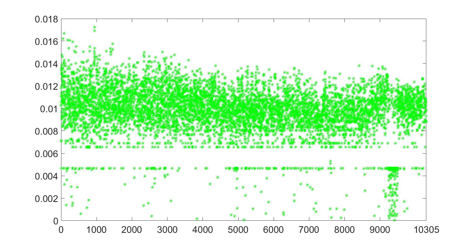 Figure 1
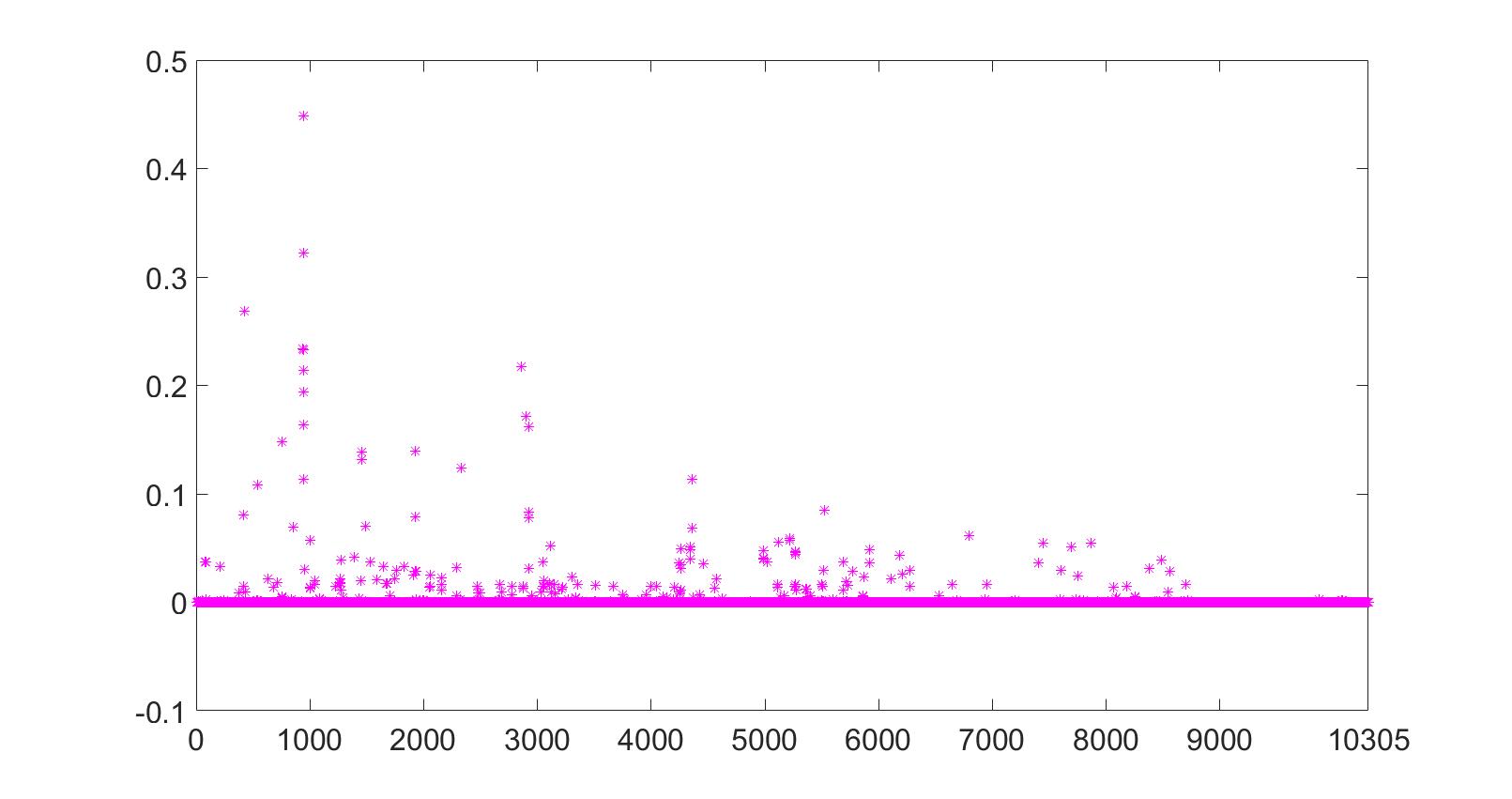 Figure 2
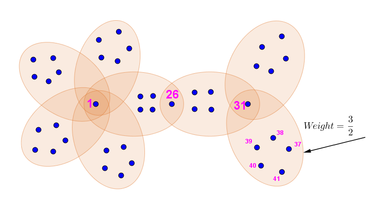 Figure 3
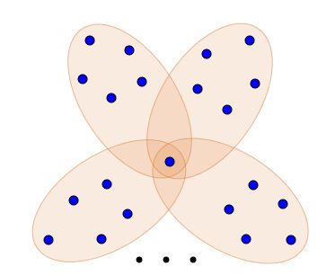 Figure 4
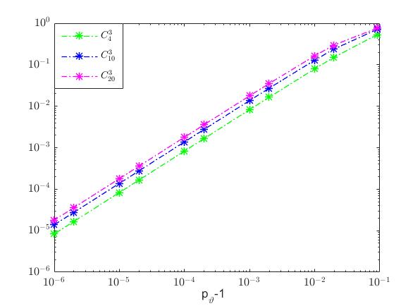 Figure 5
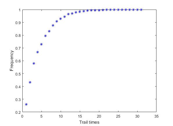 Figure 6
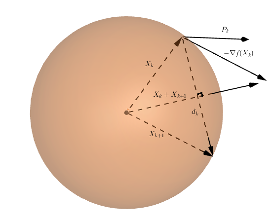 Figure 7
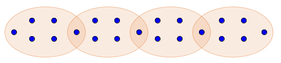 Figure 8
| Hypergraph | CSRH | SS-HOPM | ||||||
|---|---|---|---|---|---|---|---|---|
| Iter. | Time(s) | Accu. | Err. | Iter. | Time(s) | Accu. | Err. | |
| 13593 | 3.35 | 1.00 | 2668 | 4.89 | 1.00 | |||
| 1257 | 0.78 | 1.00 | 18610 | 32.58 | 0.94 | |||
| 674 | 0.42 | 1.00 | 731 | 1.61 | 1.00 | |||
| 8901 | 2.23 | 0.18 | 2317 | 4.38 | 0.22 | |||
| CSRH | CEST | ||||||||
| Iter. | Time(s) | Accu. | Err. | Iter. | Time(s) | Accu. | Err. | ||
| 3 | 4 | 38123 | 9.14 | 1.00 | 42760 | 70.28 | 1.00 | ||
| 6 | 62780 | 17.55 | 0.97 | 65706 | 105.53 | 0.99 | |||
| 8 | 71311 | 23.38 | 0.66 | 76778 | 106.95 | 0.65 | |||
| 4 | 4 | 69517 | 16.92 | 1.00 | 49331 | 79.81 | 1.00 | ||
| 6 | 86171 | 24.83 | 0.96 | 76105 | 113.11 | 0.98 | |||
| 8 | 75907 | 24.71 | 0.33 | 91690 | 106.57 | 0.42 | |||
|
|
||||||||||||||||||||||||||||||||||||||||||||||||||||||||||||||||||||||||||||||||||||||||
| Iter. | Time(s) | Accu. | Err. | |
|---|---|---|---|---|
| 3037 | 0.99 | 1.00 | ||
| 13271 | 17.88 | 1.00 | ||
| 51018 | 110.53 | 1.00 | ||
| 84848 | 88.85 | 1.00 |
| Ranking | ||||||
|---|---|---|---|---|---|---|
| Num. | Val. | Num. | Val. | Num. | Val. | |
| 1 | 39 | 0.4082483175 | 41 | 0.4081204985 | 1 | 0.1709715830 |
| 2 | 38 | 0.4082482858 | 39 | 0.4081204985 | 31 | 0.1678396311 |
| 3 | 31 | 0.4082482855 | 31 | 0.4081204983 | 26 | 0.1618288319 |
| 4 | 41 | 0.4082482854 | 38 | 0.4081204982 | 39 | 0.1600192388 |
| 5 | 40 | 0.4082482849 | 40 | 0.4081204973 | 38 | 0.1600192387 |
| 6 | 37 | 0.4082482834 | 37 | 0.4081204958 | 41 | 0.1600192387 |
| 7 | 24 | 0.0000000000 | 28 | 0.0073198868 | 40 | 0.1600192386 |
| 8 | 34 | 0.0000000000 | 30 | 0.0073192175 | 37 | 0.1600192385 |
| 9 | 23 | 0.0000000000 | 26 | 0.0073061265 | 23 | 0.1550865094 |
| 10 | 3 | 0.0000000000 | 29 | 0.0071906282 | 22 | 0.1550865094 |
| Ranking | Author Name | ||
|---|---|---|---|
| MultiRank | |||
| 1 | Zheng Chen | Wei-Ying Ma | C. Lee Giles |
| 2 | Wei-Ying Ma | Zheng Chen | Philip S. Yu |
| 3 | Qiang Yang | Jiawei Han | Wei-Ying Ma |
| 4 | Jun Yan | Philip S. Yu | Zheng Chen |
| 5 | Benyu Zhang | C. Lee Giles | Jiawei Han |
| 6 | Hua-Jun Zeng | Jian Pei | Christos Faloutsos |
| 7 | Weiguo Fan | Christos Faloutsos | Bing Liu |
| 8 | Wensi Xi | Yong Yu | Johannes Gehrke |
| 9 | Dou Shen | Qiang Yang | Gerhard Weikum |
| 10 | Shuicheng Yan | Ravi Kumar | Elke A. Rundensteiner |
Peer Reviews
No public reviews on file for this paper yet. If you reviewed it on a platform where reviews are public (OpenReview, ICLR, NeurIPS, ICML), you can paste yours below so the community can read it here.
Videos
No videos yet. Explain this paper in a talk, walkthrough, or lecture? Add one.
Taxonomy
TopicsTensor decomposition and applications · Sparse and Compressive Sensing Techniques · Image and Signal Denoising Methods
Computing the -Spectral Radii of Uniform Hypergraphs with Applications
Jingya Chang School of Mathematics and Statistics, Zhengzhou University, Zhengzhou 450001, China and Department of Applied Mathematics, The Hong Kong Polytechnic University, Hung Hom, Kowloon, Hong Kong ([email protected]). This author’s work was partially supported by the National Natural Science Foundation of China (grant No. 11401539 and 11571178)
Weiyang Ding Department of Applied Mathematics, The Hong Kong Polytechnic University, Hung Hom, Kowloon, Hong Kong ([email protected]). This author’s work was partially supported by the Hong Kong Research Grant Council (Grant No. C1007-15G).
Liqun Qi Department of Applied Mathematics, The Hong Kong Polytechnic University, Hung Hom, Kowloon, Hong Kong ([email protected]). This author’s work was partially supported by the Hong Kong Research Grant Council (Grant No. PolyU 501913, 15302114, 15300715, 15301716 and C1007-15G).
Hong Yan Department of Electronic Engineering, City University of Hong Kong, Kowloon, Hong Kong ([email protected]). This author’s work was partially supported by the Hong Kong Research Grants Council (Grant No. C1007-15G).
Abstract
The -spectral radius of a uniform hypergraph covers many important concepts, such as Lagrangian and spectral radius of the hypergraph, and is crucial for solving spectral extremal problems of hypergraphs. In this paper, we establish a spherically constrained maximization model and propose a first-order conjugate gradient algorithm to compute the -spectral radius of a uniform hypergraph (CSRH). By the semialgebraic nature of the adjacency tensor of a uniform hypergraph, CSRH is globally convergent and obtains the global maximizer with a high probability. When computing the spectral radius of the adjacency tensor of a uniform hypergraph, CSRH stands out among existing approaches. Furthermore, CSRH is competent to calculate the -spectral radius of a hypergraph with millions of vertices and to approximate the Lagrangian of a hypergraph. Finally, we show that the CSRH method is capable of ranking real-world data set based on solutions generated by the -spectral radius model.
Key words. Eigenvalue, hypergraph, large scale tensor, network analysis, pagerank, -spectral radius.
AMS subject classifications. 05C65, 15A18, 15A69, 65F15, 65K05, 90C35, 90C53
1 Introduction
With the emergence of big data in various field of our social life, it becomes significant and challenging to analyze the massive data and extract valuable information from them. Hypergraph, as an extension of graph, provides an efficient way to represent complex relationships among objects in applied science, such as chemistry [37, 33], computer science [24, 56, 30], and image processing [5, 19, 11]. The spectral hypergraph theory has been widely studied in [14, 29, 32, 42, 53, 65, 67], which reveal combinatorial and geometric structures of hypergraphs. Moreover, spectral hypergraph approaches are useful tools to address issues in real world. Spectral hypergraph partitioning and spectral hypergraph clustering have broad applications in network analysis [43, 59], image segmentation [18], multi-label classification [61], machine learning [68], and data analysis [2, 40]. Hypergraph spectral hashing techniques highly contribute to problems of similarity search and retrieval of social image [69, 41].
In this paper, we focus on the computation of -spectral radii of uniform hypergraphs. The -spectral radius of a hypergraph was introduced in [32] and linked with extremal hypergraph problems. Extremal graph theory, as a branch of graph theory, is one of the most attractive and best studied area in combinatorics. Turán [63] introduced the famous Turán graph and Turán theorem in 1941, when is regarded as the start of the extremal graph theory. Naturally, the question was extended from graph to hypergraph in [64] that is to find the largest number of edges in a hypergraph which is -free111 A uniform hypergraph that does not have a subgraph isomorphic to the uniform hypergraph is said to be -free.. Although the Turán-type problem is adequately complete for ordinary graphs, cases are much more challenging when it comes to hypergraph. In [48], Nikiforov proved the spectral Turán-type inequality which generalized the Turán theorem. In [32], the -spectral version of Nikiforov’s inequality and the -spectral version of a hypergraph Turán result were given, and it was showed that this result can be employed in solving ‘degenerate’ Turán-type problems. Furthermore, it was proved that the edge extremal problems are asymptotically equivalent to the extremal -spectral radius problems in [49].
The -spectral radius of a hypergraph covers not only the number of edges in extremal problems, but also the notions, such as Lagrangian, and the spectral radius of a hypergraph [42]. When , the -spectral radius of a hypergraph turns out to be its Lagrangian. The Lagrangians of graph and hypergraph were proposed in [44] to prove the Turán’s theorem for graphs. The Largrangians of hypergraphs were used to disprove the conjecture of Erdös [20, 22] and to find non-jumping numbers for hypergraphs [23, 54, 55]. Also, the Lagrangian of a hypergraph is associated with problems of determining Turán densities of hypergraphs [6, 31, 45, 60], which is an asymptotic solution to a (non-degenerate) Turán problem. When , the -spectral radius of a uniform hypergraph is the largest Z-eigenvalue [57] of its adjacency tensor. When is even and equals the order of this hypergraph, the -spectral radius becomes the largest H-eigenvalue of the adjacency tensor of . Therefore, the -spectral radius is connected with the (adjacency) spectral radius of a hypergraph [27, 39, 42]. Additionally, Kang et al. provided solutions to several -spectral radius related extremal problems in [29]. Nikiforov in [50] did a comprehensive study and obtained many theoretical conclusions about -spectral radius.
Apart from the application in extremal hypergraph theory, the -spectral radius model constructs a framework to quantify the importance of objects or centrality in networks. Evaluating the significance or popularity of objects is a significant problem in data mining. It can be used to determine the importance of web pages [52, 36, 16], forecast customer behaviour [38], retrieve images [28] and so on. In the -spectral radius model, entries of the vector associated with the -spectral radius of a hypergraph are called -optimal weighting and represent the significance of its corresponding vertices. The ranking result varies when changes. We will explain the meaning of different ranking results and show the numerical performance of our algorithm in sorting real-life data in Section 6.
Calculation of -spectral radii of hypergraphs is related to several methods for evaluating tensor eigenvalues. Algorithms for tensor eigenvalues, such as the shifted symmetric higher-order power method (SS-HOPM) in [34], the generalized eigenproblem adaptive power (GEAP) method in [35], an extension of Collatz’s method (NQZ) in [46], and the CEST method, can be employed when equals 2 or when equals the order of an even-uniform hypergraph. When is even, the -spectral radius problem is equivalent to the generalized tensor eigenvalue problem [9, 17]. Therefore, methods for this generalized tensor eigenvalue problem, such as the polynomial optimization related algorithm for finding all real eigenvalues of a symmetric tensor given by Cui et al. in [15], and the homotopy approach for all eigenpairs of general real or complex tensors proposed by Chen et al. in [10] can be employed to compute even -spectral radius of small scale hypergraphs. However, the problem of computing -spectral radii of arbitrary hypergraph is still open. This is the main motivation of our paper.
To solve the -spectral radius problem, we introduce a spherically constrained maximization model, which is equivalent to the original problem. Then we use an effective conjugate gradient method to acquire an ascent direction for the constrained optimization model. Next, we employ the Cayley transform to project the ascent direction on the unit sphere. It is proved that there exists a positive parameter in the curvilinear line search such that the Wolfe conditions hold. Based on the above foundation, we propose a numerical method for computing -spectral radii of hypergraphs (CSRH) with When the CSRH method is able to approximate the -spectral radii (Largrangians) of hypergraphs. In the convergence analysis, we prove that the CSRH algorithm is convergent and it converges to the global optimization point with high probability. Numerical experiments show that CSRH is preponderant when compared to existing methods for computing Z-eigenvalues and H-eigenvalues of adjacency tensors. Moreover, CSRH is capable of calculating -spectral radii of hypergraphs with millions of vertices effectively. In addition, we find that the significance of vertices of hypergraphs is related to the order of elements of the -optimal weighting. Therefore, we apply the CSRH method to rank the vertices of the corresponding hypergraph from different viewpoints when is different, which is useful in network analysis. As an example, we show that our numerical results agree with the observed data of a small weighted hypergraph. Furthermore, we successfully rank 10305 authors based on their publication information by establishing a hypergraph model and using CSRH to solve the corresponding -spectral radius problem. We sort the authors from the view of individual and group respectively. The result of our ranking can be reasonably explained and are in line with the existing consequences in [47].
The paper is organized as follows. In Section , we introduce mathematical notions. The computational issues about -spectral radius are addressed in Section , where our new method CSRH for computing -spectral radii of hypergraphs is given. In Section , we analyze the convergent property of the CSRH method. The numerical experiments are represented in Section In Section we show the application of CSRH method in network analysis. The ranking results of a toy example and a large scale real-world problem are presented. Finally, we draw conclusions in Section .
2 Preliminary
In this section we introduce useful notions and important results on hypergraphs and tensors. Let be the th order -dimensional real-valued tensor space, i.e.,
[TABLE]
A tensor with for is said to be symmetric, if is unchanged under any permutation of indices [13]. Two operations between and any vector are defined as
[TABLE]
and
[TABLE]
Note that, and are a scalar and a vector respectively, and
If there exists a real number and a nonzero real vector satisfying
[TABLE]
then is called an H-eigenvalue of with being the associated H-eigenvector [57, 58]. Additionally, is a vector, of which the th element is When a real vector and a real number satisfy the following system
[TABLE]
is called a Z-eigenvalue of and is the corresponding Z-eigenvector [57].
Definition 2.1** (Hypergraph).**
A hypergraph is defined as , where is the vertex set and (the powerset of ) is the edge set. We call an -uniform hypergraph when for and in case of
If each edge of a hypergraph is linked with a positive number then this hyperpragh is called a weighted hypergraph and is the weight associated with the edge An ordinary hypergraph can be regarded as a weighted hypergraph with the weight of each edge being
In the rest of this paper, an -uniform hypergraph is abbreviated to an -graph for convenience and hence the hypergraph refers to an -graph. The degree of a vertex is given by The weight polynomial of [62] is defined as
[TABLE]
in which is a vector in , is an edge of and is the weight of
Definition 2.2** (-spectral radius [32, 29]).**
When , the -spectral radius of , denoted by , is defined as
[TABLE]
and we call any vector solving (2.3) a -optimal weighting of [7].
When the -spectral radius of coincides with its Lagrangian [21, 62], which is defined as
[TABLE]
The vector related to the Lagrangian of is named the optimal legal weighting [7, 62].
Definition 2.3** (Adjacency tensor ).**
The adjacency tensor of a weighted -graph is defined as an th order -dimensional symmetric tensor with its elements being
[TABLE]
It is obvious from (2.3) that the -spectral radius is exactly the product of times the largest Z-eigenvalue of the adjacency tensor , and when is even the -spectral radius is times the largest H-eigenvalue of [57].
Although there is no general formula or algorithm for us to compute the -spectral radius of a hypergraph directly, research on -spectral radius of hypergraphs with certain structures has made some progress.
Theorem 2.1** ([50]).**
*Let -graph be a -star with edges .
a. If then
b. If then
c. If then *
Proposition 2.1** ([7]).**
If is a complete -graph with vertices, then the Lagrangian of is
[TABLE]
A multiset is an extension of the ordinary set, such that the objects or elements in the multiset are repeatable. If the edge set of a hypergraph is a set of multisets, then is called a multi-hypergraph [53]. Naturally, the -spectral radius problem can be extended from hypergraph to muli-hypergraph. The algorithm and theoretical analysis in the following part of this paper are also applicable to -spectral radius problems of multi-hypergraphs. In the rest of this paper, the symbol refers to norm and the parameter is a positive integer unless stated otherwise.
3 Computation of the -spectral radius of a hypergraph
We transform the -spectral radius in (2.3) into a spherically constraint optimization problem and propose an iterative algorithm to solve it.
3.1 Spherically constraint form for
The -spectral radius of in (2.3) can be reformulated as
[TABLE]
where is the adjacency tensor of The maximization problem (3.1) is equivalent to an unconstrained format, that is
[TABLE]
In order to restrict the search region and keep the vector away from zero, we add a spherically constraint on in (3.2). Due to the zero-order homogeneous property of we can obtain by solving the following problem
[TABLE]
When , the objective function is differentiable for any nonzero and the gradient of is
[TABLE]
where represents a vector whose th element is Since is zero-order homogeneous, we have
[TABLE]
for any
Based on the spherically constrained form in (3.3), we have the following proposition, which provides a way to approximate the -spectral radius of a hypergraph when it cannot be computed directly.
Proposition 3.1**.**
Let be a sequence such that
[TABLE]
where each Then
[TABLE]
Proof.
We restrict the domain of on a unit sphere, which is denoted as Rename the function in (3.3) as
[TABLE]
and we have
[TABLE]
Here is continuous. Let be an infinite sequence on the compact space such that
[TABLE]
If there are more than one point satisfying the equation (3.8), we randomly choose one of them to be Suppose is a convergent sequence without loss of generality. Since the sequence is bounded, there exists a point satisfying
[TABLE]
For any we have
[TABLE]
from (3.8), which indicates that
[TABLE]
Then we obtain
[TABLE]
based on (3.6) and (3.9). Therefore we have Since
[TABLE]
conclusion (3.7) is then obtained.
∎
3.2 The CSRH algorithm
We employ an iterative algorithm to solve (3.3).
Suppose that the current iterate is a unit vector . Our task is to find a new iterate which satisfies the following two conditions.
is on the unit sphere; 2. 2.
is an ascent direction, i.e.,
[TABLE]
In Figure 1, the current iterate is on the unit sphere and we can see that is a unit vector if and only if the vector and the vector are perpendicular to each other, i.e.
[TABLE]
Let be a skew-symmetric matrix, i.e., Then we have
[TABLE]
Therefore, the equation (3.13) is feasible and the first condition of holds when
[TABLE]
Furthermore, based on the optimization techniques it is available to find an ascent direction such that
[TABLE]
Then the existing information in Figure 1 for us to obtain is and both of which have relation with in (3.15) and (3.5) respectively. Hence, in order to satisfy (3.12) we construct as a combination of and i.e.,
[TABLE]
and obtain
[TABLE]
Therefore, if in (3.16), is an ascent direction with .
The previous analysis shows that the two conditions of are valid when satisfies (3.14) and (3.16) for . This motivates us to construct the skew-symmetric matrix by and Let
[TABLE]
with being a positive parameter. The constant in (3.16). Since the angle between vectors and is less than or equal to in Figure 1, then we have However if i.e., there is a contradiction when we substitute by in (3.14). Hence, we have and equations (3.14) and (3.16) hold, which means the two conditions of are satisfied when is the matrix in (3.18) with being an ascent direction.
Lemma 3.1**.**
The new iterate can be expressed as
[TABLE]
from (3.14) and (3.18). Further we have
[TABLE]
Proof.
From (3.14), we obtain where
[TABLE]
That is to say the orthogonal transform is in fact the Cayley transform. The proof is then similar to Lemma in [8, 12]. ∎
For the new point in (3.19), a crucial step is to find an ascent direction to guarantee the ascent property in (3.15). Since problems related with hypergraphs and tensors are often large and time-consuming for computation, we employ the nonlinear conjugate gradient method, which is proposed for large-scale nonlinear optimization problems, to acquire a suitable . The nonlinear conjugate gradient method does not need the Hessian matrices of the objective function and is usually faster than the steepest descent method. In [25, 26], a nonlinear conjugate gradient method called CGDESCENT was given and it was proved that the CGDESCENT possesses a good descent property. Attracted by this merit, we adopt the construction of parameter in CGDESCENT and obtain the ascent direction by
[TABLE]
The scalar above is defined as , where
[TABLE]
parameters and The initial direction is chosen as The direction in (3.21) is proved to satisfy the ascent property in the following Lemma.
Lemma 3.2**.**
The search direction generated by (3.21) satisfies the sufficient ascent condition, i.e.
[TABLE]
and there exists a constant such that
[TABLE]
Proof.
When it is easy to show that the two inequalities hold. For we have
[TABLE]
Since
[TABLE]
we obtain
[TABLE]
Then we deduce that
[TABLE]
Inequality (3.24) is valid when ∎
In the curvilinear line search, the parameter in (3.19) is determined to ensure that the Wolfe conditions hold. We provide the details in the next subsection.
3.3 Feasibility of Wolfe conditions
In this section we prove that there exists a step length satisfying the Wolfe conditions for the curvilinear search in (3.19) in each iteration. First, we compute the derivative of which plays an important role in line search.
Lemma 3.3**.**
Let be the derivative of at point Then we have
[TABLE]
Proof.
Equation (3.19) means that
[TABLE]
Then we take derivative with respect to as follows
[TABLE]
By multiplying both sides of (3.26) by we get
[TABLE]
from (3.19). Since from (3.27) we obtain
[TABLE]
∎
Since is twice continuously differentiable in the compact set , we can find a constant such that
[TABLE]
For a given optimization algorithm which enjoys a good ascent or descent property, it is proved that step lengths that satisfy the Wolfe conditions exist for a monotonous line search in [51, Lemma 3.1]. In the following theorem we prove that Wolfe conditions are practicable for the curvilinear line search in our algorithm.
Theorem 3.1**.**
If , there exists satisfying
[TABLE]
Proof.
Let and From (3.19), we have and
[TABLE]
Denote a linear function Then and due to and in (3.23). Since is bounded above, the graph of must intersect with the line at least once when . Suppose is the smallest intersection point, we obtain
[TABLE]
By the mean value theorem, we can find satisfying
[TABLE]
On the other hand, from (3.5) and (3.19) we have
[TABLE]
Then we have
[TABLE]
Combining (3.32) and (3.33), we have
[TABLE]
Further, from (3.31) we obtain
[TABLE]
Combing (3.34) and (3.35) we have
[TABLE]
Since
[TABLE]
and , we have
[TABLE]
Since ,
[TABLE]
Since , inequality (3.30) holds when Also from the condition , we have and (3.29) is obtained. ∎
Up to now, the algorithm CSRH for computing the -spectral radius of a hypergraph is available. First we transform the original model of into an equivalent constrained optimization problem on the unit sphere (3.3). To solve the constrained model, we compute the ascent direction from (3.4), (3.22) and (3.21), and choose a proper so that the next iterate gained via (3.19) satisfies the Wolfe conditions (3.29) and (3.30). A fast computation method for calculating and was proposed in [8], which improves the efficiency of products of adjacency tensor and vector. We also adopt this technique in our algorithm.
4 Convergence analysis
In this section we prove that the CSRH algorithm converges to a stationary point of and touches the exact -spectral radius with a high probability. Our CSRH algorithm terminates finitely when there exits a constant such that The following convergence analysis is for the case that the sequence is infinite and is always a nonzero vector.
4.1 Convergence results
Next theorem shows that CSRH algorithm is convergent.
Theorem 4.1**.**
Suppose the sequence is generated by the algorithm CSRH from any . Then we have
[TABLE]
Proof.
The demonstration is divided into two steps. First, we show that the Zoutendijk condition holds, i.e.,
[TABLE]
Here is the angle between and , which is denoted as
[TABLE]
Since is bounded, we have is Lipschitz continuous on , i.e.,
[TABLE]
for a constant . From (3.18), we have
[TABLE]
Hence from (3.14)
[TABLE]
[TABLE]
From (3.30), we obtain
[TABLE]
By using the above two relations, we can derive the inequality
[TABLE]
which implies
[TABLE]
Then from (3.29), we obtain
[TABLE]
which derives the following inequality
[TABLE]
Since is bounded in (3.28), the inequality (4.1) is then deduced.
Next, we show that the angle is bounded away from . By combining (3.23) and (3.24), we obtain
[TABLE]
The above inequalities indicate that
[TABLE]
Therefore, from (4.1) we have
[TABLE]
∎
Recall that the graph of a function is defined as
[TABLE]
For the function involved in our problem (3.3), we have
[TABLE]
where and are positive integers. Since is a semialgebraic set, is a semialgebraic function and satisfies the Łojasiewicz inequality [1, 4, 66], which means that for a critical point of , there exist constants and , as well as being a neighbourhood of such that
[TABLE]
for The next theorem shows that if the sequence is infinite, it has a unique accumulation point.
Theorem 4.2**.**
Assume the infinite sequence is generated by the CSRH algorithm. Then it converges to a unique point that is,
[TABLE]
and is a first-order stationary point.
Proof.
From (4.5), (3.23) and (3.24) we have
[TABLE]
Moreover, from (3.29) and (3.23) we obtain
[TABLE]
We take no account of condition under which the algorithm terminates finitely. The above inequality indicates that
[TABLE]
Based on (3.24), (3.29) and (4.3), we have
[TABLE]
From (4.9) and (4.10), as well as the Łojasiewicz inequality (4.7), we have the conclusions hold based on [1, Theorem 3.2]. ∎
4.2 Probability of obtaining the exact -spectral radius
Due to the feasibility of Łojasiewicz inequality in (4.7), we get the probability of the CSRH method touching the true -spectral radius.
Proposition 4.1** ( ).**
Suppose CSRH algorithm is implemented from uniformly distributed initial points on for times. We take the largest one among the results of these trails as the -spectral radius of the relevant problem. The probability of getting the exact -spectral radius is
[TABLE]
in which is a constant satisfying If is large enough, the probability is high.
Proof.
This Proposition can be proved in the way similar to [8, Theorem 4.9]. We omit the details. ∎
5 Numerical experiments
In this section, we show the performance of CSRH for computing -spectral radii of both small and large scale hypergraphs. We compare our method with several existing methods for computing eigenvalues of adjacency tensors. Examples of approximating the Lagrangian of a hypergraph are given in Subsection 2. All experiments are carried out by using MATLAB version R2015b and Tensor Toolbox version 2.6 [3]. The experiments in Subsections 5.1 and 5.2 are terminated when
[TABLE]
where is our computed -spectral radius and is the exact result obtained from theorems or conclusions in existing literature. The maximum iteration of CSRH is taken as 1000 for all algorithms except those performed by the MATLAB function in Tensor Toolbox. For each experiment in this section, we compute 100 times to obtain 100 estimated values and choose the largest one as our computational result of the -spectral radius related with . When is attainable, the accuracy rate of the CSRH algorithm is defined as
[TABLE]
Each number of iterations (Iter.) and computational time (Time) we reported in this section is the sum of corresponding quantities for all 100 executions of the experiment. The relative errors (Err.) between the numerical results and the exact solutions are provided.
5.1 Computation of -spectral radii of hypergraphs
We compare the following three algorithms for computing eigenvalues of adjacency tensors associated with different hypergraphs:
- •
An adaptive shifted power method [34] SS-HOPM. This method can be invoked by eig_sshopm in Tensor Toolbox 2.6 for Z-eigenvalues of symmetric tensors.
- •
A first-order optimization algorithm CEST [8] which is proposed for eigenvalues of large scale sparse tensors involving even order hypergraphs.
- •
CSRH: the method proposed in Section 3.
Example 1 (). First, we compute the largest Z-eigenvalues of adjacency tensors of the following hypergraphs:
[TABLE]
The first hypergraph is given in [65] as Example 1, while the last three hypergraphs are Example and in [53]. The hypergraph is actually a tetrahedron.
In Table 1, we demonstrate results of CSRH and SS-HOPM for computing the largest Z-eigenvalues of adjacency tensors of some small hypergraphs. Since all the four hypergraphs given above are of odd orders, the comparison does not include CEST method, which is designed for even order hypergraphs. The Err. column shows the relative error between the computational result and the exact largest Z-eigenvalue provided in the corresponding references. Under the condition that the relative error reaches , our CSRH method is much more stable and efficient than the SS-HOPM method.
In the next experiment, we study the probability of CSRH method getting the true largest Z-eigenvalue of and show that the probability increases along with the trail times. We employ the CSRH method to compute the largest Z-eigenvalue of the adjacency tensor of from uniformly distributed and randomly chosen initial points. Once the relative error between the computational largest Z-eigenvalue and its exact value reaches the experiment is terminated and we record the number of trails. This experiment is repeated for one thousand times. Let be the total occurrence of experiments whose trail time is the integer The frequency of touching the exact Z-eigenvalue when running times is
[TABLE]
In Figure 2, we display the relation between trail times and success probability. It illustrates that the probability tends to one along with the increase of trail times which coincides with the conclusion in Theorem 4.1.
Example 2 (). Next, we compare CEST and CSRH methods for computing the largest H-eigenvalues of adjacency tensors of loose paths. An -graph with edges is called a loose path if its vertex set is
[TABLE]
and its edge set is
[TABLE]
An -uniform loose path with edges has vertices. For example, the -unform loose path with edges in Figure 3 has vertices.
The following theorem proved in [67] offers a convenient way to acquire the largest H-eigenvalues of adjacency tensors of loose paths with or .
Theorem 5.1** ([67]).**
Let be an -uniform loose path with edges and be the largest H-eigenvalue of its adjacency tensor . Then we have
\lambda_{H}(G)=\big{(}\frac{1+\sqrt{5}}{2}\big{)}^{\frac{2}{r}}* for * 2. 2.
* for *
In Table 2, we compare CSRH and CEST for computing the largest H-eigenvalues of adjacency tensors of different loose paths. The column Err. presents the relative error between our computed result and the exact one given by Theorem 5.1. When relative error achieves precision of the CSRH method saves at least of the time CEST takes in every problem. The comparison between CEST and CSRH verifies that the high efficiency of CSRH method does not only relies on the fast computation technique in [8], because CEST method use this technique as well.
Example 3. If all edges of a hypergraph share a same vertex, then it is called a -star. An -uniform -star with edges have vertices.
We present a class of -uniform -star in Figure 4 as an example.
We calculate -spectral radii of -stars with various orders and edges and display the results in Table 3. The Err. column presents the relative error between our computational result and the corresponding exact result generated from Theorem 2.1. It can be seen that all tests succeed with high accuracy rates. Even the -spectral radii and -spectral radii of -stars with millions of vertices are gained with high probability and efficiency.
5.2 Approximation of Lagrangians of hypergraphs
When the -spectral radius is also known as the Lagrangian of a hypergraph (2.4). However, is not smooth at who has some zero elements. We use to approximate , with being denoted as
[TABLE]
Since we have from Proposition 3.1. Therefore, we can use -spectral radius to approximate the Lagrangian of a hypergraph. The function is continuous and differentiable and CSRH method is feasible for computing -spectral radius of a uniform hypergraph. Let be a vector such that its th element being
[TABLE]
Then function is also a semialgebraic function and satisfies the Łojasiewicz inequality (4.7). Therefore, the conclusions in Section 4 hold for in (5.3).
In this subsection, we show the results of CSRH method approximating Lagrangian of a hypergraph. First we give an example to demonstrate that the CSRH method is competent to compute the -spectral radius of a uniform hypergraph when is a fraction in (5.3). Next, the numerical results of approximating the Lagrangians of complete hypergraphs by -spectral radius are represented. The termination criteria of algorithms in the remaining part of this paper is set as
In Table 4, we present the consequences of the -spectral radius of a 3-uniform -star with 10 edges, with being the fraction in the first column. The true -spectral radius can be acquired from Theorem 2.1. All experiments produce the exact -spectral radius with probability and the relative error between our numerical result and the theoretical value obtained from Theorem 2.1 is at most
An -uniform hypergraph is said to be complete if it contains all possible edges when the number of its vertices is fixed. We use to denote a complete -graph with vertices. Then the 3-graph is actually a tetrahedron with 6 edges. The Lagrangian of a complete uniform hypergraph can be obtained directly from Proposition 2.1.
We compute different -spectral radii of 3 complete hypergraphs , and . In Figure 5, the ordinate reflects the error between the -spectral radius and the true Lagrangian of the corresponding complete hypergraph which is obtained from the Proposition 2.1, while the abscissa means the value of When approaches to the -spectral radius is close to the exact Lagrangian of the related hypergraph.
6 Network analysis
Not only the -spectral radii, i.e., the optimal value of in (3.3), but also the optimal point in (3.3) characterize the structure of hypergraphs. Recall (2.3) that an optimal point is called a -optimal weighting. The elements of the -optimal weighting reflect the importance of the corresponding vertices in the hypergraph. Therefore, we may call the th element of the -optimal weighting the impact factor of the th vertex. Different selections of the parameter provide different criteria of the importance of the vertices. When is relatively large, the criterion tends to evaluate the importance of vertices more individually. When is relatively small, the ranking result demonstrates the significance of groups of vertices. In this section, we compute each -spectral radius 10 times and choose the vector corresponding to the largest value as the -optimal weighting.
6.1 A toy problem
We first employ a toy problem to illustrate the impact of the selections of . We construct a 6-uniform weighted hypergraph with 8 edges as in Figure 6. The weights of all edges of this hypergraph are set as , except the last one whose weight is . Obviously from the hypergraph, the vertices numbered , , and are distinct from other vertices, and the edge is also distinct from other edges. In Table 5, we show the different ranking of vertices via different -optimal weighting. The abbreviation Num. means the number of a vertex and Val. represents the impact factors of the corresponding vertices.
When the top vertices are in the edge who has the only largest weight among all edges. From Table 5, we can see that the impact factor of the top vertices in the -optimal weighting are much greater than others. In fact, the value of all impact factors, except those corresponding to the top vertices, are less than which means that the dominant vertices are the ones from the largest weighted edge and the others can be ignored. That is to say, the ranking in this case offers the most important group of the vertices. When , the vertex numbered appears in the top 10 list and the difference among the top impact factors is not as great as that when . When , the top vertices are , , and the impact factors of vertices that have same status in the hypergraph are rather close to each other. Then, we believe that the ranking results of -spectral radius reflects the significance of vertices individually.
6.2 Author ranking
Ng et al. in [47] collected publication information from DBLP222http://www.informatik.uni-trier.de/ ley/db/ and gave different rankings of the authors according to different factors, such as citations of authors, category concepts, collaborations, and papers. In this subsection, we use the same data set in [47] and rank the authors based on their collaborations.333We would like to thank Dr. Xutao Li for providing the database.
We construct a weighted 3-uniform multi-hypergraph with edges to store the cooperation information. The vertex set is composed of numbers of the 10305 authors and each edge has 3 vertices indicating that these three authors have cooperations under a same topic. The weight of an edge is decided by the collaboration times among the three authors in this edge. The adjacency tensor of this multi-hypergraph is a sparse tensor with nonzero entries.
The example in Subsection shows that we can obtain the ranking score from different viewpoints by computing different -optimal weighting. Therefore, we compute -optimal weighting and -optimal weighting of to get the author group ranking and the author ranking respectively. In Figure 7(a), the stars stand for the -optimal impact factors of vertices of Obviously, the majority elements of -optimal weighting are extraordinarily close to zero and only dozens of corresponding stars are above the horizontal line of In fact, of the entries in the -optimal weighting are less than and the elements that are greater than occupy only On the other hand, the largest impact factor reaches to and the upper stars are considerably larger than others. It means that the -optimal weighting is dominated by a small proportion of its components and we regard these leading elements as a group. The top ten authors ranked according to the 2-optimal impact factor are presented in the second column of Table 6. The average collaboration times of each two authors among these top ten authors are which is far larger than , the average collaboration times of each two authors among the whole authors. Since these top ten authors have intimate cooperation, it is rational to consider them as a group and interpret the ranking in the second column as the most powerful group.
Stars in Figure 7(b) are the -optimal impact factors of vertices of The distribution of these stars is totally different from the ones in Figure 7(a). It can be seen in Figure 7(b) that the -optimal impact factors of the authors are uniform and most of them are concentrated in the internal between and Because in the original data set, the collaboration times of different authors are mostly one or two and we rank the authors based on their collaborations, the balance and concentration of the impact factors match up with the cooperation information. The top ten authors generated via the -optimal impact factors are listed in the third column of Table 6. Ng et al. also ranked the authors in the light of collaboration times and the influence of category concepts of their publications. We demonstrate the top 10 authors of their experimental result [47] in the MultiRank column in Table 6. It can be seen that of the top authors in the MultiRank are coincident with results of our -optimal rank.
7 Conclusions
We convert the -norm constraint in -spectral radius problem into an orthogonal constraint, and propose a first order iterative algorithm CSRH for solving it. In this method, it is feasible to obtain a proper step length to satisfy the Wolfe conditions under the curvilinear line search. Convergence analysis shows that the CSRH method is globally convergent. The iterates converges to a -optimal weighting. Numerical experiments show that CSRH method is efficient and powerful. In the author ranking application problem, we construct a weighted hypergraph with millions of edges. By computing -spectral radius of this hypergraph, the most influential cooperation group and the top ten ranked authors are presented.
The reference list from the paper itself. Each links out to its DOI / PubMed record.
- 1Absil et al. [2005] P.-A. Absil, R. Mahony, and B. Andrews. Convergence of the iterates of descent methods for analytic cost functions. SIAM J. Optim. , 16(2):531–547, 2005.
- 2Agarwal et al. [2005] S. Agarwal, J. Lim, L. Zelnik-Manor, P. Perona, D. Kriegman, and S. Belongie. Beyond pairwise clustering. In 2005 IEEE Computer Society Conference on Computer Vision and Pattern Recognition (CVPR’05) , volume 2, pages 838–845. IEEE, 2005.
- 3Bader et al. [2015] B. W. Bader, T. G. Kolda, et al. Matlab tensor toolbox version 2.6. Available online, February 2015. URL http://www.sandia.gov/~tgkolda/Tensor Toolbox/ .
- 4Bolte et al. [2006] J. Bolte, A. Daniilidis, and A. Lewis. The Łojasiewicz inequality for nonsmooth subanalytic functions with applications to subgradient dynamical systems. SIAM J. Optim. , 17(4):1205–1223, 2006.
- 5Bretto and Gillibert [2005] A. Bretto and L. Gillibert. Hypergraph-based image representation. In International Workshop on Graph-Based Representations in Pattern Recognition , pages 1–11. Springer, 2005.
- 6Brown and Simonovits [1984] W. Brown and M. Simonovits. Digraph extremal problems, hypergraph extremal problems, and the densities of graph structures. Discrete Math. , 48(2-3):147–162, 1984.
- 7Caraceni [2011] A. Caraceni. Lagrangians of hypergraphs, 2011. URL http://alessandracaraceni.altervista.org/My Wordpress/wp-content/uploads%/2014/05/Hypergraph_Lagrangians.pdf . [Online; accessed 26-January-2017].
- 8Chang et al. [2016] J. Chang, Y. Chen, and L. Qi. Computing eigenvalues of large scale sparse tensors arising from a hypergraph. SIAM J. Sci. Comput. , 38(6):A 3618–A 3643, 2016.