Bridging Perturbative Expansions with Tensor Networks
Laurens Vanderstraeten, Micha\"el Mari\"en, Jutho Haegeman, Norbert, Schuch, Julien Vidal, Frank Verstraete

TL;DR
This paper introduces a tensor network framework that reformulates perturbative expansions in quantum many-body systems, enabling better interpolation across phase transitions and revealing order parameters for topological phases.
Contribution
It presents a novel tensor network approach to perturbative expansions, connecting them with entanglement properties and phase transition indicators in quantum systems.
Findings
Tensor networks effectively interpolate perturbative expansions.
Constructed perturbative entanglement Hamiltonians with spectral insights.
Tensor networks reveal order parameters for topological phase transitions.
Abstract
We demonstrate that perturbative expansions for quantum many-body systems can be rephrased in terms of tensor networks, thereby providing a natural framework for interpolating perturbative expansions across a quantum phase transition. This approach leads to classes of tensor-network states parametrized by few parameters with a clear physical meaning, while still providing excellent variational energies. We also demonstrate how to construct perturbative expansions of the entanglement Hamiltonian, whose eigenvalues form the entanglement spectrum, and how the tensor-network approach gives rise to order parameters for topological phase transitions.
Click any figure to enlarge with its caption.
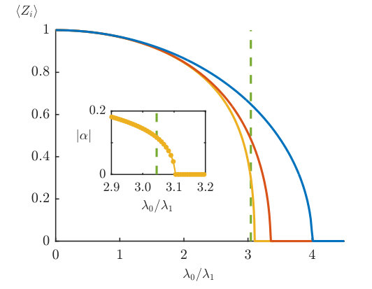 Figure 1
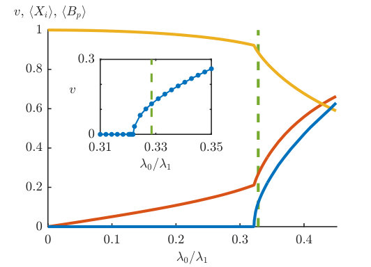 Figure 2
Peer Reviews
No public reviews on file for this paper yet. If you reviewed it on a platform where reviews are public (OpenReview, ICLR, NeurIPS, ICML), you can paste yours below so the community can read it here.
Videos
No videos yet. Explain this paper in a talk, walkthrough, or lecture? Add one.
Bridging Perturbative Expansions with Tensor Networks
Laurens Vanderstraeten
Department of Physics and Astronomy, Ghent University, Krijgslaan 281, S9, 9000 Gent, Belgium
Michaël Mariën
Department of Physics and Astronomy, Ghent University, Krijgslaan 281, S9, 9000 Gent, Belgium
Jutho Haegeman
Department of Physics and Astronomy, Ghent University, Krijgslaan 281, S9, 9000 Gent, Belgium
Norbert Schuch
Max-Planck-Institut für Quantenoptik, Hans-Kopfermann-Str. 1, 85748 Garching, Germany
Julien Vidal
Laboratoire de Physique Théorique de la Matière Condensée, CNRS UMR 7600, Université Pierre et Marie Curie, 4 Place Jussieu, 75252 Paris Cedex 05, France
Frank Verstraete
Department of Physics and Astronomy, Ghent University, Krijgslaan 281, S9, 9000 Gent, Belgium
Vienna Center for Quantum Science and Technology, Faculty of Physics, University of Vienna, Boltzmanngasse 5, 1090 Vienna, Austria
Abstract
We demonstrate that perturbative expansions for quantum many-body systems can be rephrased in terms of tensor networks, thereby providing a natural framework for interpolating perturbative expansions across a quantum phase transition. This approach leads to classes of tensor-network states parametrized by few parameters with a clear physical meaning, while still providing excellent variational energies. We also demonstrate how to construct perturbative expansions of the entanglement Hamiltonian, whose eigenvalues form the entanglement spectrum, and how the tensor-network approach gives rise to order parameters for topological phase transitions.
In the last decade, interest in two-dimensional strongly correlated quantum systems has increased considerably, mainly due to the existence of exotic quantum behavior and topological order. The strong quantum correlations and entanglement patterns that characterize these systems give rise to, e.g., topologically protected ground states Wen and Niu (1990); Bravyi et al. (2010) and anyonic excitations Wilczek (1982); Kitaev (2006), which can be used to manufacture reliable quantum memories and perform fault-tolerant quantum computation Freedman et al. (2003); Ogburn and Preskill (1999); Wan . However, the entanglement properties that allow for these nontrivial properties also make these systems very hard to simulate, as mean-field approaches fail to capture the essential quantum correlations and quantum Monte Carlo simulations often suffer from the sign problem.
Perturbation theory has proven successful in studying the robustness of topological phases (see Ref. Dusuel et al. (2011) for instance), but such an approach necessarily fails when approaching a transition point. Indeed, quantum phase transitions naturally disconnect different perturbative descriptions, so that the critical properties cannot be captured easily. A complementary approach is the variational method, which does not inherently break down at criticality. In that respect, much progress has been obtained using tensor-network states Verstraete et al. (2008); Orús (2014), although it remains a matter of debate to what extent variational calculations correctly describe the phase of a given model Balents (2014).
This paper proposes a method that combines the perturbative and variational approaches. The central idea is to represent the perturbative expansions of the ground state in the tensor-network formalism, lift the perturbative coefficients to variational parameters, and apply the tensor-network machinery to variationally optimize the energy density. This approach allows to merge distinct perturbative expansions in a single variational wave function, and to bridge between perturbative series expansions on both sides of a critical point.
General framework— Let us start with standard perturbation theory for a Hamiltonian . At order one, in the limit where , the (unnormalized) perturbed ground state of is given by
[TABLE]
where and . For many-body systems, such expressions do not have the extensivity structure expected for a ground-state wave function. If is a sum of local interactions, the perturbative correction creates a zero-momentum superposition of local excitations rather than a finite density of excitations on top of the unperturbed reference state . The exponentiated form , instead, does give rise to an extensive wave function by automatically incorporating all disconnected Feynman diagrams. An elegant way of obtaining such an expression is via the formalism of quasiadiabatic time evolution Hastings and Wen (2005), which shows that perturbation theory can be cast into a low-depth quantum circuit acting on a reference state Acoleyen et al. (2016).
Starting from the two unperturbed states and , we can construct a one-parameter path interpolating between these two states, connect both perturbative expansions into a single wave function
[TABLE]
and consider as variational parameters. The variational optimization requires us to compute the energy expectation value accurately, a task that might seem more easy using the original expression of Eq. (1). However, because of the nonextensivity, Eq. (1) generically yields a zero variational contribution, a dilemma pointed out by Feynman Feynman (1984). Here, we rely on the low-depth quantum circuit representation of Eq. (2) and use tensor-network methods to compute the corresponding expectation values. In fact, the formalism of tensor networks Verstraete et al. (2008) provides a direct way to build extensive wave functions that match, order by order, a given perturbative expansion. Indeed, according to the linked-cluster theorem, in order to represent increasing orders in perturbation theory, we need to apply clusters of local operators of increasing size on our reference state. These clusters can be efficiently encoded in a tensor-network operator Pirvu et al. (2010), so that, if the reference state itself can be represented as a tensor-network state, we can construct states similar to the one in Eq. (2) in an efficient way.
In two dimensions this construction gives rise to projected entangled-pair states F. Verstraete and J. I. Cirac (PEPSs), for which efficient algorithms exist Vanderstraeten et al. (2016) to optimize the variational parameters directly in the thermodynamic limit. The computational complexity of the tensor-network construction is determined by the so-called bond dimension , which scales linearly in the number of clusters (this number typically scales exponentially in the order of perturbation theory). Because we only have a small number of parameters, the variational optimization can be performed with high precision and does not introduce systematic errors.
Additionally, rephrasing perturbation theory in terms of tensor networks gives rise to a description of correlations in terms of an auxilliary space encoding the entanglement degrees of freedom. This allows us to determine a perturbative expansion of the entanglement Hamiltonian Cirac et al. (2011), whose eigenvalues represent the entanglement spectrum Li and Haldane (2008).
Transverse-field Ising model— Let us illustrate our approach with the ferromagnetic transverse-field Ising model (TFIM) on a square lattice defined by
[TABLE]
Here, and denote the usual Pauli matrices acting on site . This model is known to exhibit a phase transition between a polarized phase and a symmetry-broken phase detected by the magnetization along the direction. The critical point is located at as estimated by Monte Carlo simulations Blöte and Deng (2002). Let us note that the ground-state manifold of is twofold degenerate but, since for any finite in the thermodynamic limit, we can safely use the procedure described above (in the following, denotes the polarized state in the direction).
For this problem, we choose the one-parameter reference state
[TABLE]
which is a simple product state interpolating between the unique ground state at and one of the symmetry-broken ground states at . If one only considers as an order-zero variational ansatz, one finds a critical point at , which is the standard mean-field result.
Next, we consider the first- and second-order perturbative expansions in terms of tensor-network operators acting on and . The wave function corresponding to those expansions can be represented as a PEPS with bond dimension . In the limit , we can reproduce the first-order perturbative wave function by a simple tensor-network operator. When acting on the unperturbed state , it gives rise to a PEPS with bond dimension . Although not exactly equal to the exponentiated operator, this state reproduces the correct perturbative wave function up to first order. Because of its extensivity, the operator also creates disconnected pairs of clusters in second order, but we need to introduce two new entries in our tensor network in order to account for the next-nearest-neighbour clusters . This results in the tensor network operator listed in Table 1, which can reproduce the perturbative expansion up to second order when acting on . A similar construction can be done starting from the ferromagnetic state , where second-order perturbation theory yields .
A key feature is that both of those tensor networks with can be implemented as a single tensor network with bond dimension . The perturbative coefficients can then be lifted to variational parameters to provide an ansatz wave function with five variational parameters, two () corresponding to the first-order expansion, two () for second order and one () for the reference state on which the tensor-network operator acts (see Table 2).
Using this ansatz and the techniques developed in Ref. Vanderstraeten et al. (2016) to minimize the energy, we computed the optimal parameters as a function of . The ground-state magnetization as a function of the magnetic field is shown in Fig. 1. The order-one ansatz yields a critical transition at , whereas one gets for the order-two ansatz. These results show that we can compute the phase diagram of the TFIM with a good precision by systematically adding quantum fluctuations on top of the mean-field state as suggested by perturbation theory. Interestingly, the -symmetry breaking is solely determined by defined in Eq. (3), so that this parameter can also be considered as a reliable “virtual order parameter” (see inset in Fig. 1).
Entanglement Hamiltonians— Our perturbative PEPS wave function now allows us to define an entanglement Hamiltonian, which we illustrate by considering the perturbative expansion around the polarized state as defined by the tensors in Table 1. The entanglement Hamiltonian is defined as , where and are the leading left and right eigenvectors of the quantum transfer matrix associated with the PEPS Cirac et al. (2011). In the present case, the transfer matrix is real symmetric, and can easily be obtained perturbatively. In second order (see Table 1) we obtain a density matrix of a spin-1/2 chain:
[TABLE]
where is the projector onto the polarized state in the direction acting on site , and . By using the expansion
[TABLE]
we find that the entanglement Hamiltonian:
[TABLE]
reproduces the above expression for up to second order in . It is fascinating that we obtain a nearest-neigbor XY spin chain in a transverse magnetic field that reproduces the perturbative expansion for the entanglement spectrum around the polarized state.
Our framework now also enables a perturbative calculation of the entanglement entropy for e.g. a bipartion of an infinitely long cylinder with circumference into two half-infinite cylinders; we find the result
[TABLE]
Toric code in a magnetic field— The second example we consider is the toric code Kitaev (2003) in a magnetic field. The phase diagram of this model has been the subject of many studies for various directions of the field Hamma and Lidar (2008); Trebst et al. (2007); Vidal et al. (2009a, b); Tupitsyn et al. (2010); Dusuel et al. (2011). Here, for simplicity, we consider the case where the field points in the direction. This model, called the TCX model in the following, is defined as
[TABLE]
Degrees of freedom are spin 1/2 living on the links of a square lattice. Vertex and plaquette operators are defined by
[TABLE]
where products are performed over all sites belonging to vertex and plaquette , respectively. As early realized Hamma and Lidar (2008); Trebst et al. (2007), the TCX model can be mapped onto the TFIM if one restricts to the (charge-free) sector where . It is easy to see that the ground state belongs to this sector for all and . For the system is in a polarized phase, whereas for the system is in a topologically ordered phase that strongly contrasts with the symmetry-broken phase of the TFIM. The mapping onto the TFIM exchanges and so that the transition point of the TCX is found at .
Following Ref. Dusuel and Vidal (2015), we choose as a reference state
[TABLE]
For , is the polarized ground state of , whereas, for , is a ground state (among four under periodic boundary conditions) of . Let us note that, contrary to the TFIM, given in Eq. (7) is not a product state (except for ), but an entangled state described by a PEPS with bond dimension Verstraete et al. (2006). From a variational point of view, both models are thus very different. Using only , one finds a transition for Dusuel and Vidal (2015), in analogy with the TFIM.
We can now repeat the same procedure as before and include quantum fluctuations on top of this mean-field state as inspired by perturbation theory. For the case of second-order perturbation theory, this leads to a PEPS with bond dimension with fifteen free parameters. As for the TFIM, defined in Eq. (7) can be considered as a virtual order parameter. Indeed, at order zero, it has been shown in Ref. Dusuel and Vidal (2015) that the topological entanglement entropy Kitaev and Preskill (2006); Levin and Wen (2006) is only nonvanishing for . More generally, the concept of injectivity Schuch et al. (2010) allows us to characterize the topological content of our variational states by identifying the entanglement symmetry that is realized on the virtual level of the tensor-network operator. Away from , this virtual symmetry is explicitly broken, but also for the virtual symmetry can be broken spontaneously Schuch et al. (2013); Haegeman et al. (2015); Duivenvoorden et al. . Both explicit and spontaneous breaking of the virtual symmetry, and thus of the physical topological order, can be detected by a suitable order parameter evaluated on the virtual level of the tensor network. For the case at hand, we find that the variational solution favors explicit symmetry breaking, which we quantify as , where represents the nontrivial operation on the virtual level sup . In Fig. 2, we have plotted this virtual order parameter as a function of , as well as the expectation values of the relevant operators in and . We observe that the phase transition is signaled by a sharp onset of the virtual order parameter, and we estimate the transition point at .
Conclusions— In this paper, we have used insights from perturbation theory to motivate a variational ansatz for the description of ground states of perturbed Hamiltonians in two-dimensional spin systems in the thermodynamic limit. This ansatz is a subset of PEPS, but contains only a handful of parameters related to operators whose presence is expected from perturbation theory. Crucially, we have shown that the ansatz manages to smoothly interpolate between perturbative expansions on either side of a critical point. In addition, our approach gives access to (i) a virtual order parameter, which, in the absence of symmetry breaking, signals a topological phase transition, and (ii) the entanglement spectrum of perturbative wave functions giving rise to an explicit construction of the entanglement Hamiltonian.
Our method is generally applicable to quantum lattice models for which one can write down perturbative expansions. In the case of the square-lattice Heisenberg model, where the first-order perturbative expansion starting from the Ising limit can be written as a PEPS with bond dimension , we have observed that this one-parameter family of states gives rise to the same variational energy as a full -PEPS simulation for the isotropic Heisenberg point. It should be interesting to improve this result by going to higher orders in perturbation theory, connecting different perturbative expansions, and by considering other two-dimensional lattices. Furthermore, our method is particularly suited to tackle a range of topological phase transitions among which is the perturbed string-net model Levin and Wen (2005); Schulz et al. (2013, 2014); Dusuel and Vidal (2015); Schulz and Burnell (2016).
From the perspective of PEPS simulations our results are important for the following reasons. First of all, whereas the physical meaning of the variational parameters in a PEPS has always been somewhat of a mystery, the parameters in our ansatz have a clear meaning in terms of perturbative expansions. Second, from a numerical perspective such a reduced parametrization has clear advantages. Although the optimization problem is drastically reduced in size, we can still capture the critical behavior across (topological) quantum phase transitions. Also, we open up a way to apply the formalism of virtual PEPS symmetries characterizing topological phases Schuch et al. (2010); Şahinoğlu et al. ; Bultinck et al. to the variational simulation of topological phase transitions. The virtual order parameter that we have identified for the toric code model serves as a first illustration of what is possible in that direction.
Acknowledgements— We acknowledge inspiring discussions with S. Dusuel. This work was supported by the Austrian Science Fund (FWF) through grants ViCoM and FoQuS and the European Commision through SIQS and ERC grants QUTE, WASCOSYS (No. 636201) and ERQUAF (No. 715861). J.H., M.M., and L.V. are supported by the Research Foundation Flanders (FWO).
I Perturbation theory
General perturbation theory treats the Hamiltonian
[TABLE]
by writing down the wave function and ground-state energy as a series in :
[TABLE]
Expanding the Schrödinger equation in different orders gives rise to the following equations
[TABLE]
Solving the first-order equation gives the result
[TABLE]
We observe that . Solving the second-order equation gives
[TABLE]
and
[TABLE]
so that
[TABLE]
because the last two terms cancel.
Note that the state that we obtain is not normalized, but we can add a component along the unperturbed state to which makes sure that the state is normalized up to second order in :
[TABLE]
If one is not concerned with the normalization of the state , we can equally well work with the form in Eq. (18). In fact, one can always add a component along the unperturbed state to the state without this having an influence on the second-order equation [Eq. (13)].
II Tensor-network operators
In this section we explain how to build a physical wave function from a TNO, and how we can apply clusters of local operators in an extensive way. Consider thereto as the elementary building block the object which represents an operator acting on a physical spin for every input of the virtual indices (here, is the dimension of the virtual legs and is called the bond dimension of the TNO). Alternatively, we can represent as a six-leg tensor,
[TABLE]
where the up and down legs represent the action on a physical spin, and the four virtual legs correspond to the virtual indices. In Fig. 3 we have indicated how this tensor gives rise to a tensor-network operator and, when applied to a product state, gives rise to a wave function on an infinite two-dimensional lattice.
Let us now show how to encode clusters of local operators in this tensor. First of all, we can define the following entry
[TABLE]
such that the corresponding TNO can be expanded in as
[TABLE]
We can build two-site clusters of ’s by defining a new entry
[TABLE]
where these four entries are related by rotations of the tensor. The corresponding expansion of the TNO in is given by
[TABLE]
where denotes all nearest-neighbour pairs, and denotes all pairs of nearest-neighbours that do not overlap. Three-site clusters can be represented by the entries
[TABLE]
with corresponding expansions in the TNO:
[TABLE]
Here we have used and for denoting all linear and corner-shaped three-site clusters, resp. The center site of each cluster is labeled , and can correspond to a different operator .
One can imagine how larger and larger clusters can be constructed in this way. Also, by opening up more levels in the virtual indices, we can incorporate clusters of different operators in the TNO.
Note that we are never concerned with the normalization of the TNO; this is easily taken into account when optimizing the ground-state density expectation value Vanderstraeten et al. (2016).
III Transverse-field Ising model
In this section we treat the transverse-field Ising model on the square lattice,
[TABLE]
where denotes nearest-neighbour pairs of spins.
III.1 Mean-field theory
In mean-field theory we use the one-parameter family of states
[TABLE]
with a magnetization
[TABLE]
The energy density of this state is given by
[TABLE]
This function can be minimized straightforwardly for a given value of , showing that the minimum is at for , and the minimum starts to shift once . The resulting magnetization curve was plotted in the main body.
III.2 Exponentiated perturbation theory
In this section, we show explicitly how the exponentiated forms of perturbation theory reproduce the linear perturbative expansions, but can go beyond them as well. We treat both limits separately.
Around paramagnetic state— In this limit we start from and treat as a perturbation with small prefactor ; we will start from the state and do perturbation theory up to second order in . At first order, we find and the following wave function:
[TABLE]
We can exponentiate this form to obtain
[TABLE]
where we have denoted as a sum over all pairs of sites, not necessarily nearest neighbour, and . Note that each pair is summed over only once in the above expression, explaining why the factor from the expansion of the exponential has vanished. In second order, we also have a contribution where two ’s act on the same state, giving rise to a component along the unperturbed state . Since these contributions are unimportant from the variational point of view, we have omitted them from the expansion. We observe that the exponentiated form not only contains the first-order expansion, but represents large portions of higher orders in as well. Out of the region of small , we expect that this state contains more correlations than the linear form above, and therefore is a better variational state.
Let us go to second order. The second-order wave function is given by
[TABLE]
Here, represents all nearest-neighbour pairs, whereas stands for all pairs of sites that are not on neighbouring sites. Upon exponentiating, we observe that the disconnected contributions (where and are not nearest neighbours) are already contained within the first-order wave function, but we need to correct the prefactor for the last term. Therefore, we have the following exponentiated version of the second-order wave function
[TABLE]
which again matches the above linear form up to second order, but contains a lot more than that.
Around polarized state— Now we start from and treat as a perturbation with small prefactor ; we will start from the state , and derive the perturbation theory in . At first order, we find the following wave function:
[TABLE]
which we can exponentiate to obtain
[TABLE]
Here denotes all two nearest-neighbour pairs that do not have any sites in common, whereas we have used as a notation for all three-site clusters ( denotes the center site of the cluster and the cluster can take on two different shapes).
The second-order result for the wave function is given by
[TABLE]
Again, we observe that the disconnected contributions are already contained within the first-order exponentiated wave function, but we need a correction for the second term. Therefore, we have the following exponentiated version of the second-order wave function
[TABLE]
This wave function matches the above linear form up to second order – again, up to the components along the unperturbed state – but contains a lot more.
III.3 The TNO for the Ising model
In this section we explain how to represent perturbative expansions for the TFIM using TNOs. As explained above, we define a TNO by a single six-leg tensor , represented diagrammatically as
[TABLE]
The four virtual indices can take on values (i.e., the TNO has bond dimension ), whereas the up and down going legs correspond to the physical action of the tensor on a single-site spin state. The tensor thus represents a one-site operator for every specific input on the virtual level. In Table 3 we list all the different non-zero entries that we possibly need for representing the series expansions in and . Note in advance that the TNOs are not exactly the same operators as the exponentiated operators that we have introduced above, but share the same “extensive” properties. Let us follow the TNO construction in detail.
Around paramagnetic state— The first step in representing the perturbed state (35) is rather trivial. Indeed, by turning on the parameter in Table 3 we can easily represent the appearance of local operations acting on the state . The two-site clusters of operations can now be implemented by the parameter. The expansion of the TNO with these two parameters is given by
[TABLE]
This implies that the choice
[TABLE]
reproduces the linear perturbative expansion up to second order. The other parameters can make larger clusters of ’s, corresponding to higher orders of perturbation theory.
Around polarized state— Now we will also need to include three-site clusters in order to reproduce second-order perturbation theory in . These larger clusters are provided by the and parameters in Table 3. The former represents the midpoint of a corner-shaped three-site cluster, whereas the latter is responsible for making the linear clusters. In both cases the tensor entry with parameter provides the end points of the cluster. This implies that the expansion of the TNO with these three parameters is given by
[TABLE]
Here, and are corner-shaped and linear three-site clusters, resp. If we now choose the parameters
[TABLE]
we reproduce the linear wave function (40) up to second order in .
Variational parameters— The above then shows the explicit form of the TNOs that we have considered in order to produce the results in the main text. The mean-field result is obtained with the only parameter; the first-order result is obtained by keeping as variational parameters; the second-order result by keeping .
IV The Toric Code in magnetic field
The Hamiltonian is given by
[TABLE]
where
[TABLE]
We work in the subspace where is always , so we don’t consider this part of the Hamiltonian in the following.
IV.1 Mean-field theory and virtual order parameter
In order to reproduce mean-field theory for the toric code we introduce the one-parameter family of states
[TABLE]
For , we have the ground state of the model, whereas the toric-code state is obtained for . The calculations for the variational optimization of this one-parameter ansatz can be found in Ref. Dusuel and Vidal (2015).
This reference state is produced by a TNO defined by the tensor
[TABLE]
We have grouped four spins on every second vertex into one big supersite (see Fig. 4), so that the plaquette operators always act on two spins of each supersite. As before, the action of the TNO tensor depends on the inputs of the four virtual indices which can take on two different values . The different entries of the tensor are listed in Table 5. If we choose the values
[TABLE]
the TNO is exactly equal to the operator that appears in .
Also, this tensor contains the virtual order parameter. Indeed, from the framework of -injectivity we know that this TNO can give rise to a topologically ordered state only if the tensor satisfies the condition
[TABLE]
i.e., acting with ’s on the virtual indices should leave the tensor invariant ( is the usual Pauli matrix). This is the non-trivial -symmetry operation that is discussed in the main text. We define the virtual order parameter as
[TABLE]
where of a tensor just denotes the square root of the sum of all tensor entries squared. It can only be zero under the conditions
[TABLE]
which implies that the mean-field state only exhibits topological order if .
IV.2 The TNO for the Toric Code
We can capture the two second-order perturbative expansions with the TNO of bond dimension that is given in Table 5. Let us follow the construction explicitly in both limiting cases.
Around toric-code state— Suppose now that we start from the toric-code state , which is the ground state of , and we have . In second-order perturbation theory in we find
[TABLE]
where represents two sites that are not located on the same plaquette, and are two spins that share a plaquette. In order to represent this state with the TNO we turn on the three parameters , and . Indeed, the expansion in terms of these three parameters is given by
[TABLE]
where represent pairs of spin that do not live on the same supersite, represent pairs of spins that do live on the same supersite, and represent pairs of spin that live on the same plaquette. Therefore, the choice
[TABLE]
recovers the linear perturbed state up to second order in .
Around polarized state— Suppose now that we start from the fully polarized state , which is the ground state of , and we have . In second order in perturbation theory in we find
[TABLE]
where denotes a pair of neighbouring plaquettes (which don’t share any spins), denotes a pair of overlapping plaquettes (which share one common spin), and denotes a pair of disconnected plaquettes (see Fig. 5). This state can be obtained with the TNO of Table 5 up to second order in . Indeed, the parameter introduces end-points of clusters of plaquettes, whereas introduces overlapping plaquette pairs , and corresponds to neighbouring plaquette pairs (see Fig. 5). This implies the following form of the TNO:
[TABLE]
If we now we fix the parameters as
[TABLE]
we recover the linear form of the perturbed state up to second order in .
IV.3 Stacking TNOs
We can now construct a number of variational ansatz states by including, order by order, the parameters in the above TNO and applying it to the reference state . Since the reference state is itself a PEPS, the action with a TNO gives rise to a class of PEPS with bond dimension . In order to reduce this bond dimension, we introduce a slightly different construction of the variational ansatz.
The essential modification is that we include the perturbative expansion around the polarized state in the same TNO [Table 4] as the one we have used for constructing the reference state . Then, in a next step, we can apply the TNO that we need to represent the expansion around the toric-code state.
The variational ansatz that we have used to obtain the results as reported in the main body, is given by
[TABLE]
where in the definition of the tensor we have introduced the following operator on a supersite:
[TABLE]
V XXZ model
In this section, we explain how to simulate the XXZ model on the square lattice with our variational ansatz. First of all, we perform a sublattice rotation of the original model in order to arrive at the Hamiltonian
[TABLE]
This rotation maps a staggered magnetization in the and direction into a uniform one. For an exact ground state is given by
[TABLE]
whereas in first-order perturbation theory we have
[TABLE]
Since we know
[TABLE]
the wave function can be simplified to yield
[TABLE]
The TNO that gives rise to this wave function up to first order is given by a tensor given by the two entries
[TABLE]
and all rotated versions of the second entry. By interpreting the weight of the second entry as a variational parameter, we obtain the results as reported in the main text.
Note that the resulting wavefunction is -invariant, since the tensor is invariant under the generators and acting on the physical and virtual indices, respectively, while the initial Néel state provides a (staggered) background charge of per site.
The reference list from the paper itself. Each links out to its DOI / PubMed record.
- 1Wen and Niu (1990) X.-G. Wen and Q. Niu, “Ground-state degeneracy of the fractional quantum hall states in the presence of a random potential and on high-genus riemann surfaces,” Phys. Rev. B 41 , 9377 (1990) . · doi ↗
- 2Bravyi et al. (2010) S. Bravyi, M. B. Hastings, and S. Michalakis, “Topological quantum order: Stability under local perturbations,” J. Math. Phys. 51 , 093512 (2010) . · doi ↗
- 3Wilczek (1982) F. Wilczek, “Quantum mechanics of Fractional-Spin particles,” Phys. Rev. Lett. 49 , 957 (1982) . · doi ↗
- 4Kitaev (2006) A. Kitaev, “Anyons in an exactly solved model and beyond,” Ann. Phys. (NY) 321 , 2 (2006) . · doi ↗
- 5Freedman et al. (2003) M. H. Freedman, A. Kitaev, M. J. Larsen, and Z. Wang, “Topological quantum computation,” Bull. Am. Math. Soc. 40 , 31 (2003) . · doi ↗
- 6Ogburn and Preskill (1999) W. R. Ogburn and J. Preskill, “Topological Quantum Computation,” Lect. Notes Comput. Sci. 1509 , 341 (1999) . · doi ↗
- 7(7) Z. Wang, Topological Quantum Computation , CBMS Regional Conference Series in Mathematics, No. 112 (American Mathematical Society, Providence, 2010). · doi ↗
- 8Dusuel et al. (2011) S. Dusuel, M. Kamfor, R. Orús, K. P. Schmidt, and J. Vidal, “Robustness of a Perturbed Topological Phase,” Phys. Rev. Lett. 106 , 107203 (2011) . · doi ↗