Uncertainty Quantification of geochemical and mechanical compaction in layered sedimentary basins
Ivo Colombo, Fabio Nobile, Giovanni Porta, Anna Scotti, Lorenzo, Tamellini

TL;DR
This paper develops an advanced uncertainty quantification method for layered sedimentary basin evolution, incorporating multi-material properties, improved deterministic solvers, and innovative surrogate modeling techniques to handle discontinuities.
Contribution
It introduces a novel approach combining coordinate transformations and physical interface features for surrogate modeling in multi-layered basin simulations.
Findings
Accurately reproduces multi-modal probability densities of key variables.
Enhances deterministic solver efficiency with Newton method.
Effectively manages discontinuities in stochastic modeling.
Abstract
In this work we propose an Uncertainty Quantification methodology for sedimentary basins evolution under mechanical and geochemical compaction processes, which we model as a coupled, time-dependent, non-linear, monodimensional (depth-only) system of PDEs with uncertain parameters. While in previous works (Formaggia et al. 2013, Porta et al., 2014) we assumed a simplified depositional history with only one material, in this work we consider multi-layered basins, in which each layer is characterized by a different material, and hence by different properties. This setting requires several improvements with respect to our earlier works, both concerning the deterministic solver and the stochastic discretization. On the deterministic side, we replace the previous fixed-point iterative solver with a more efficient Newton solver at each step of the time-discretization. On the stochastic side,…
Click any figure to enlarge with its caption.
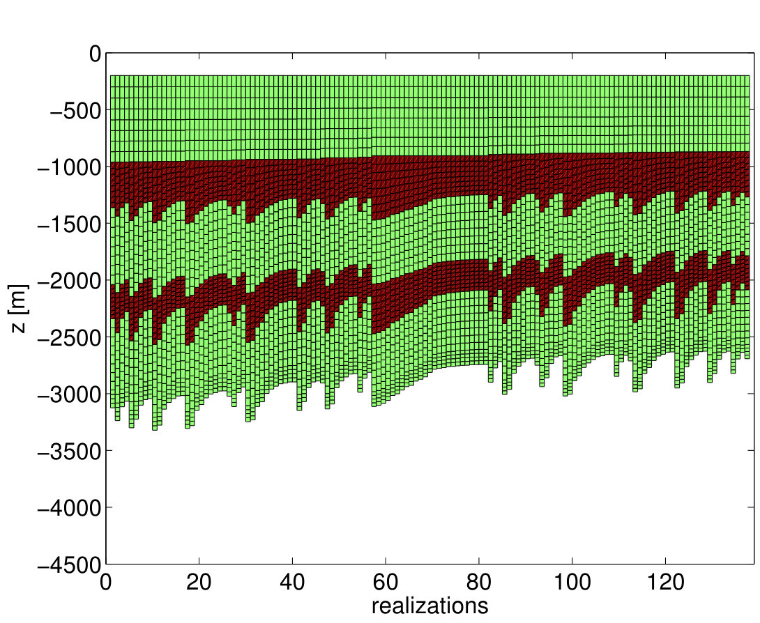 Figure 1
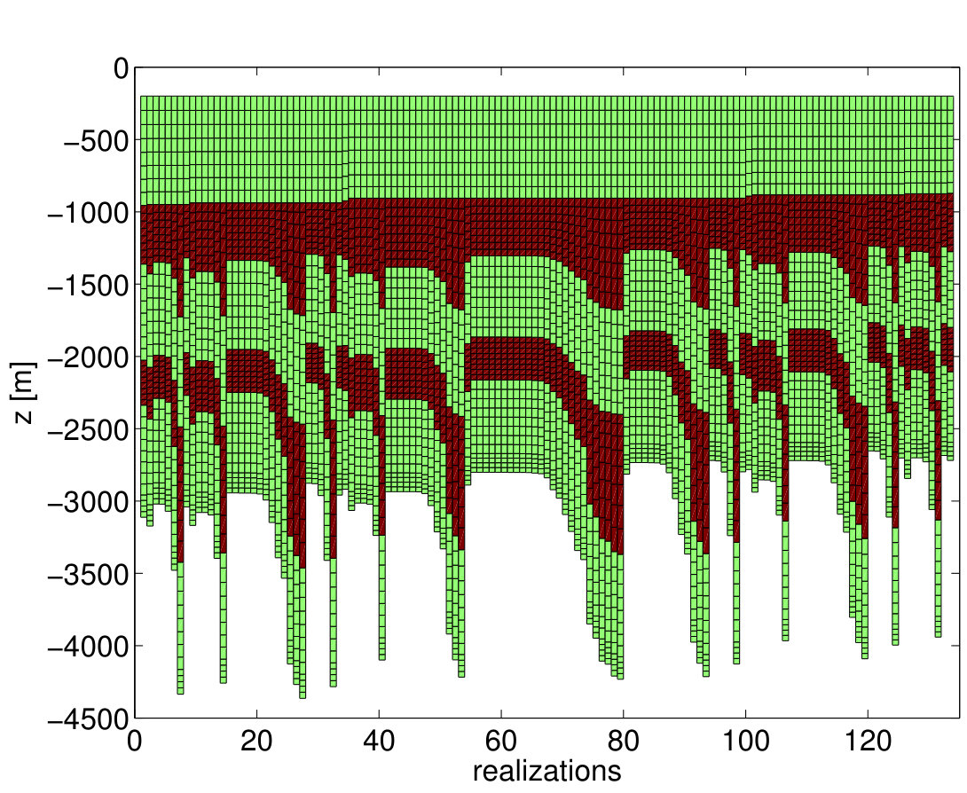 Figure 2
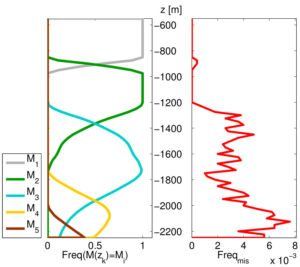 Figure 3
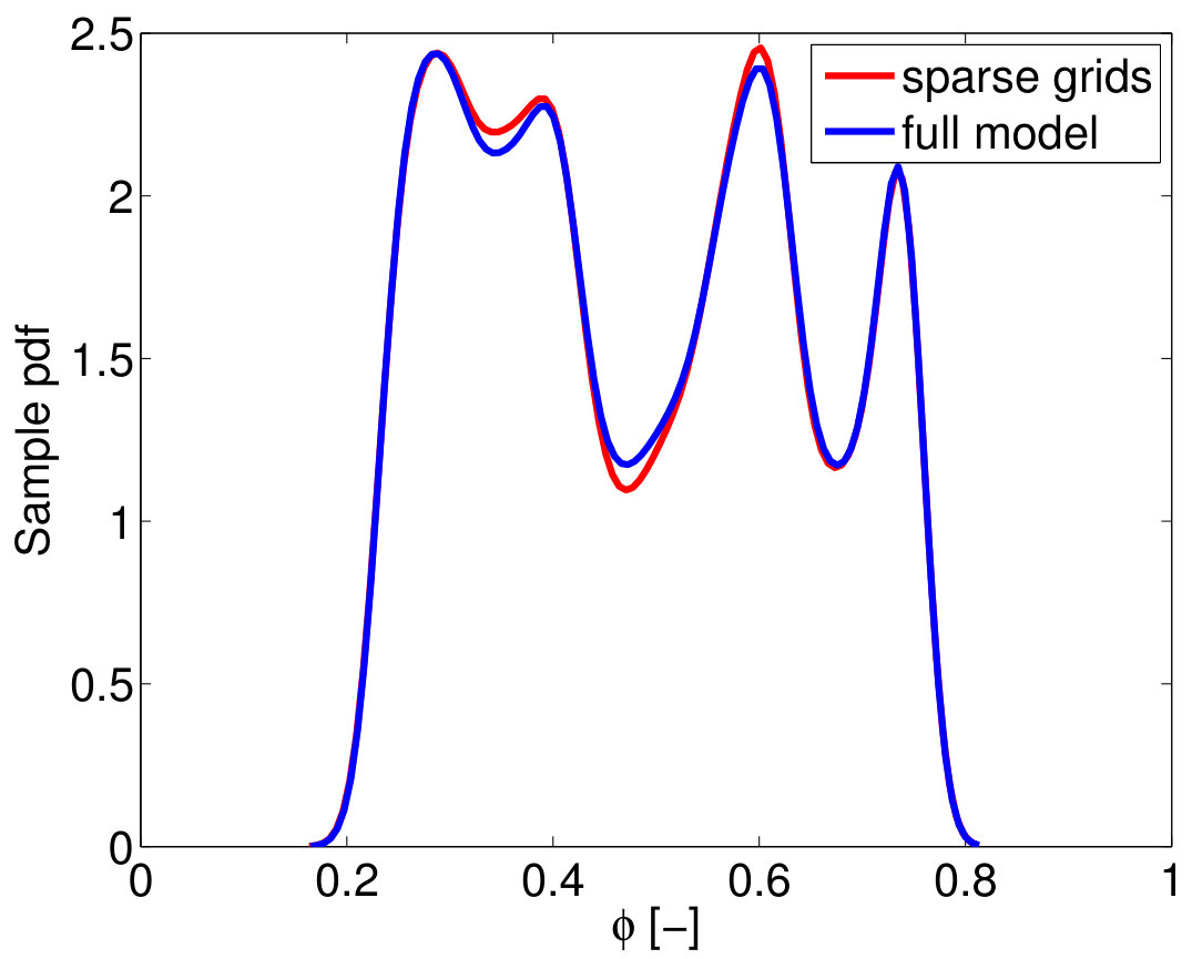 Figure 4
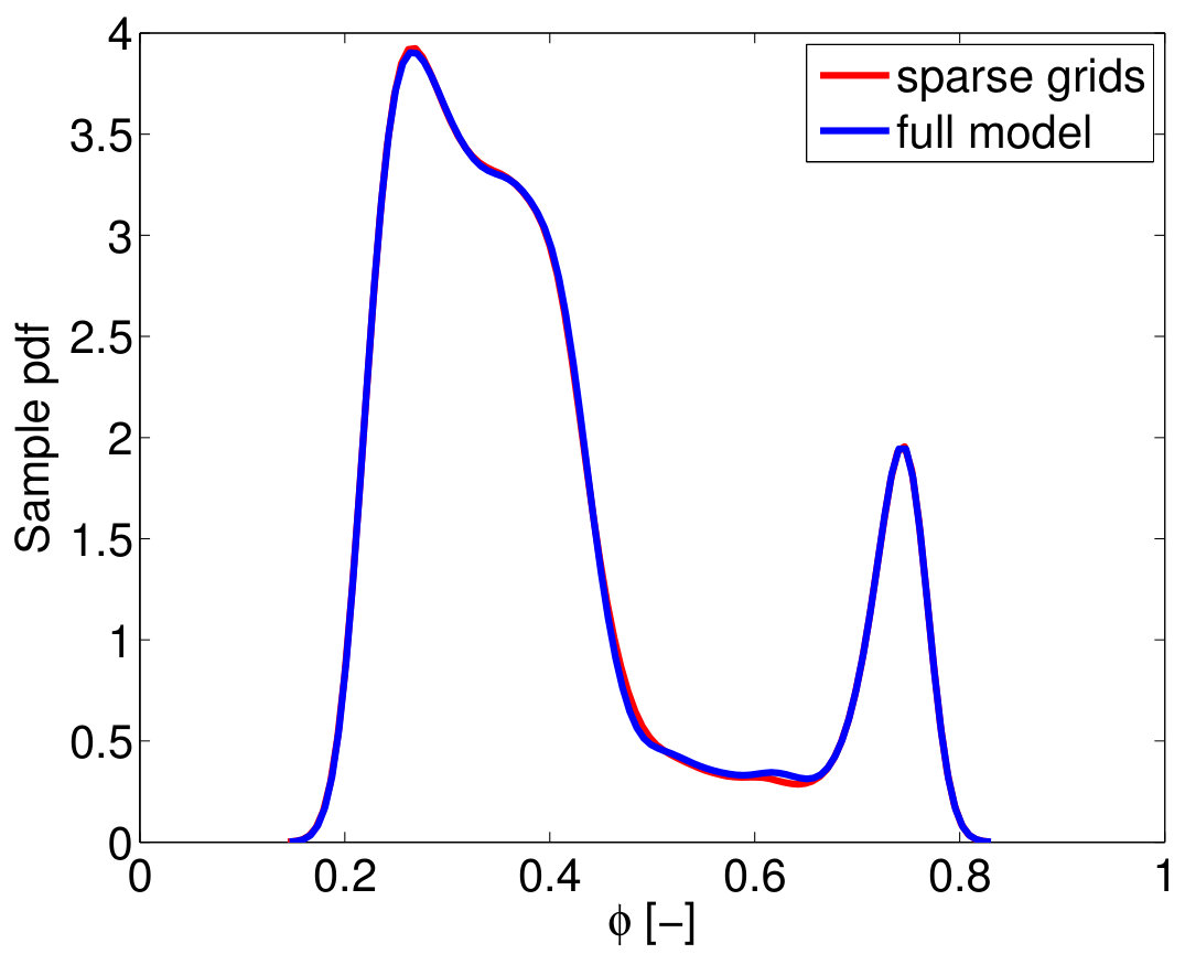 Figure 5
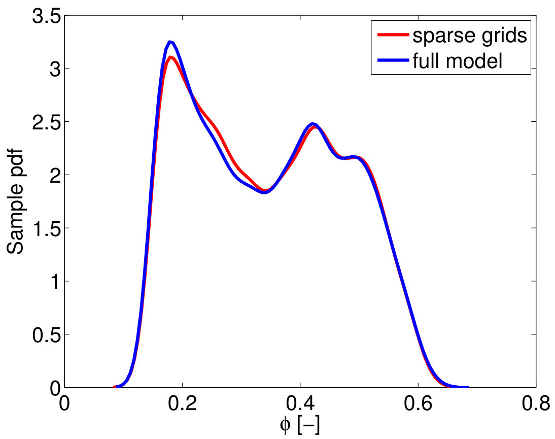 Figure 6
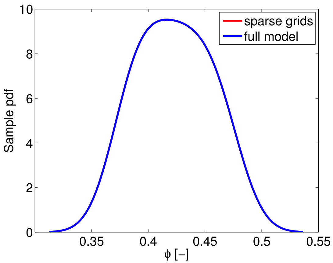 Figure 7
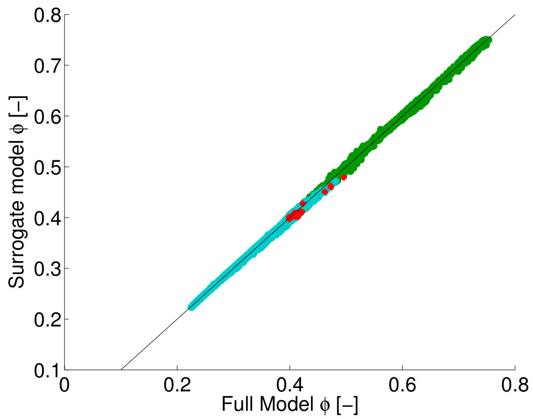 Figure 8
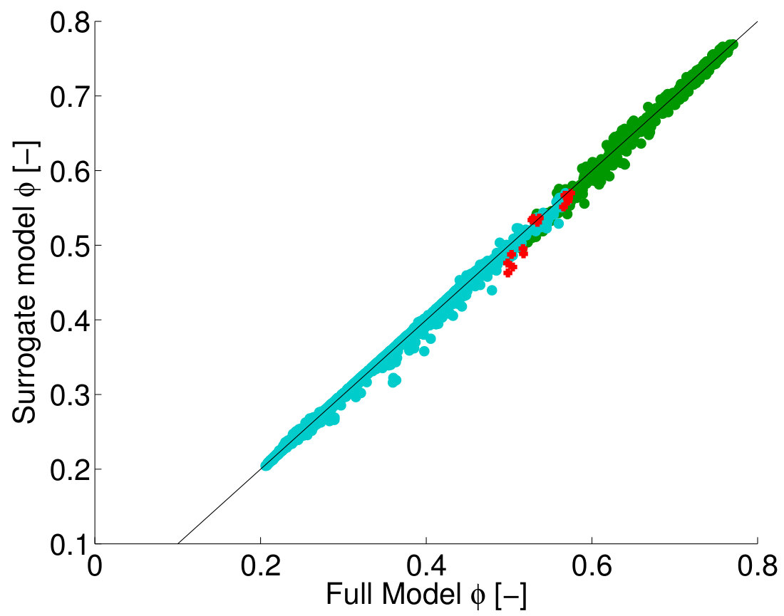 Figure 9
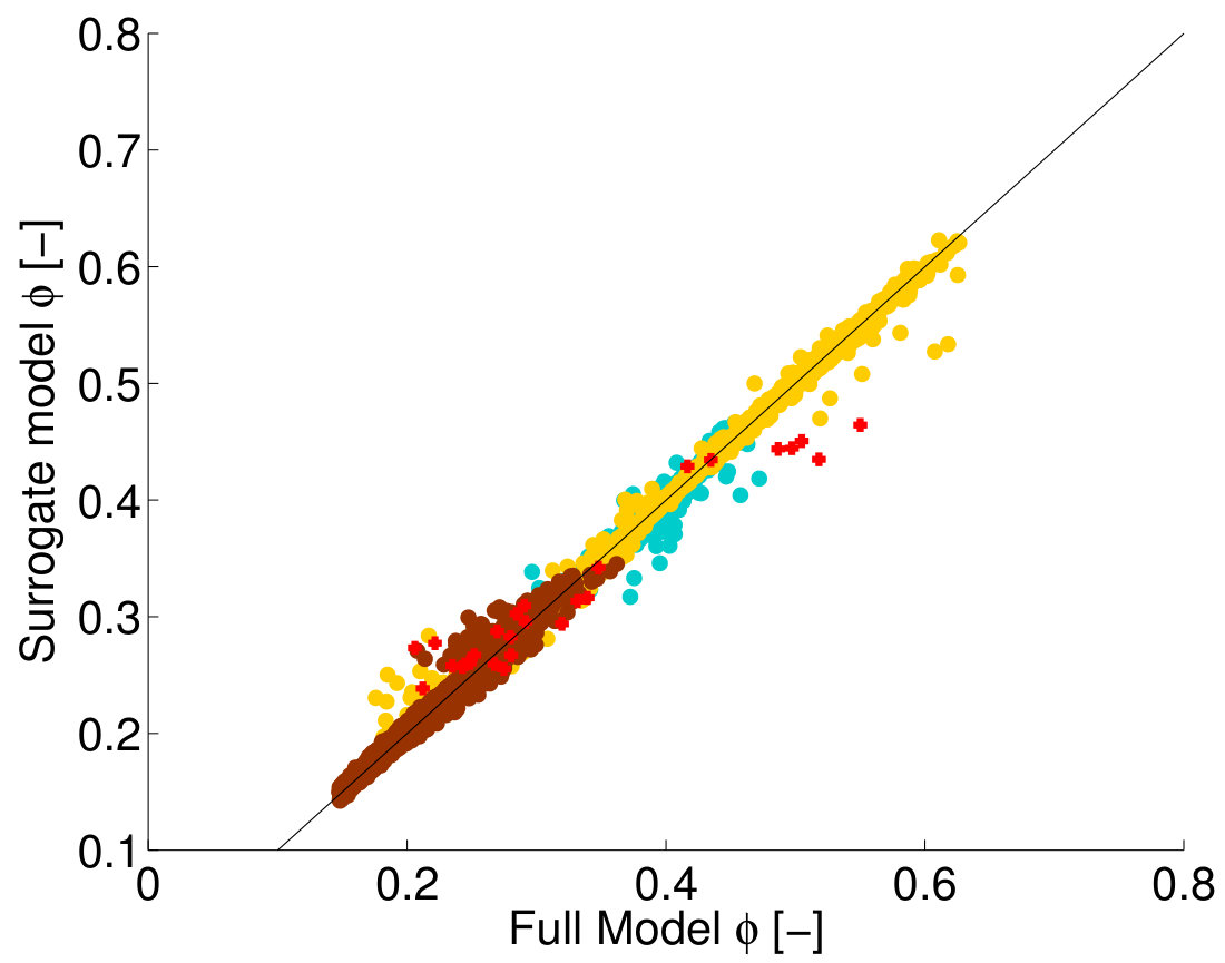 Figure 10
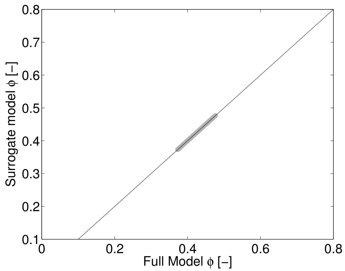 Figure 11
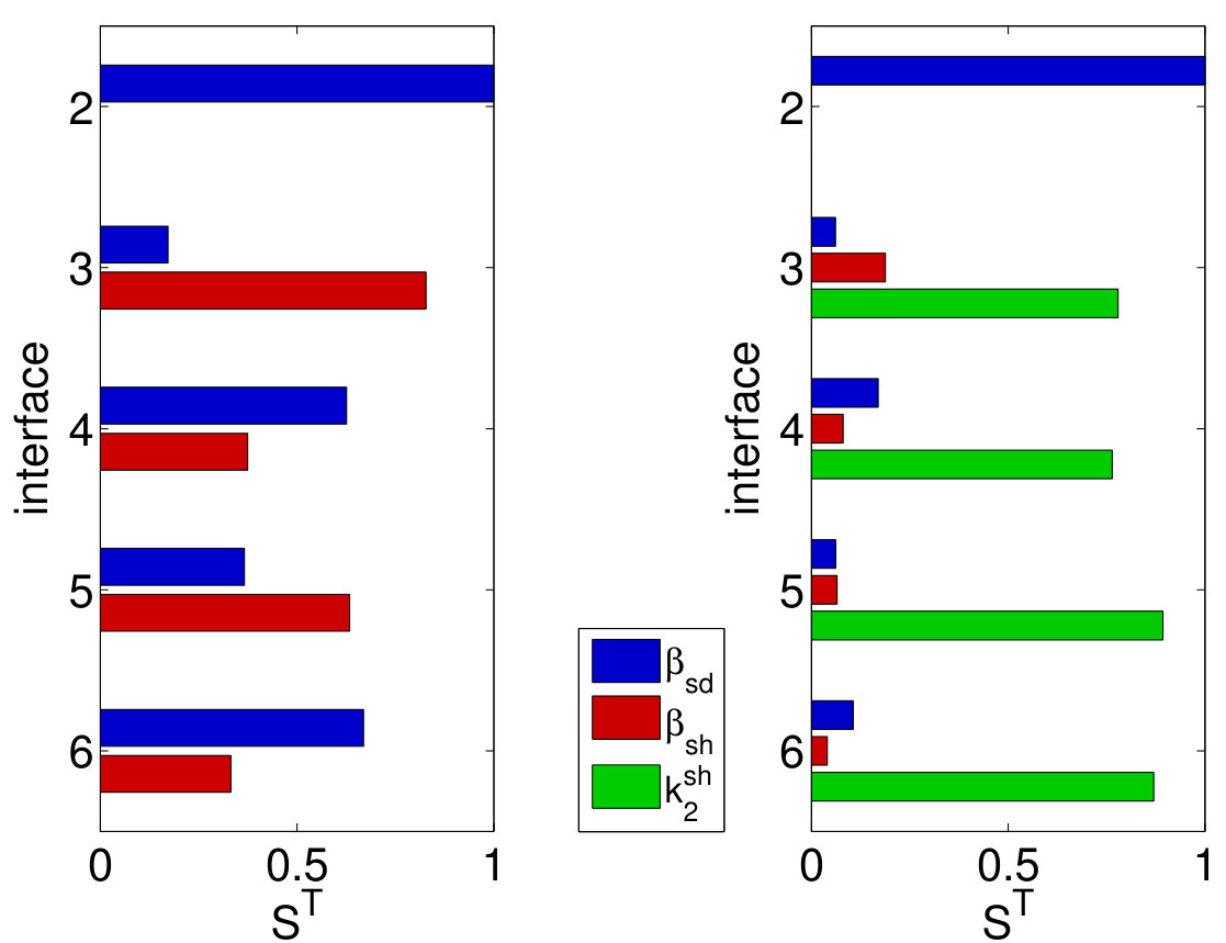 Figure 12
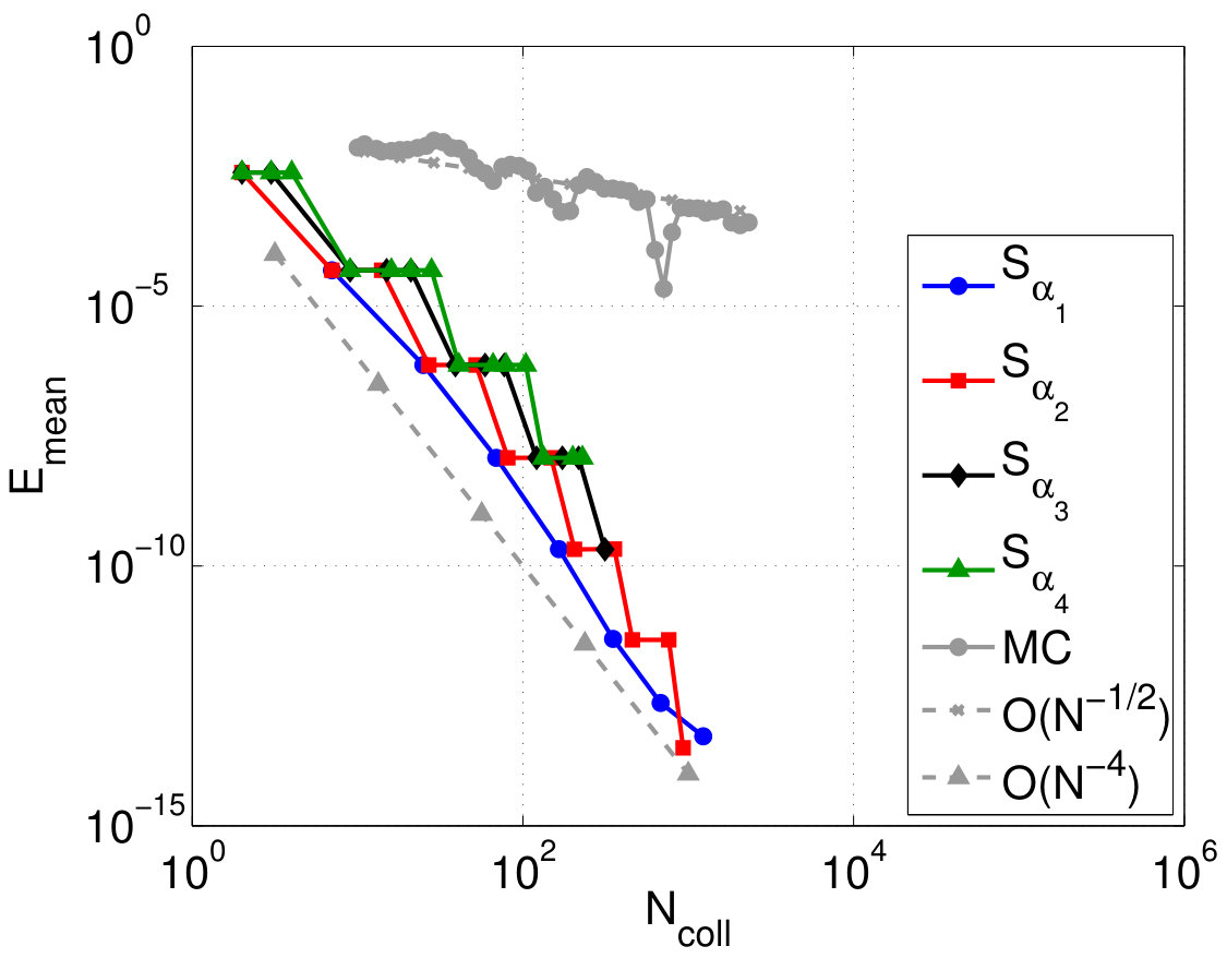 Figure 13
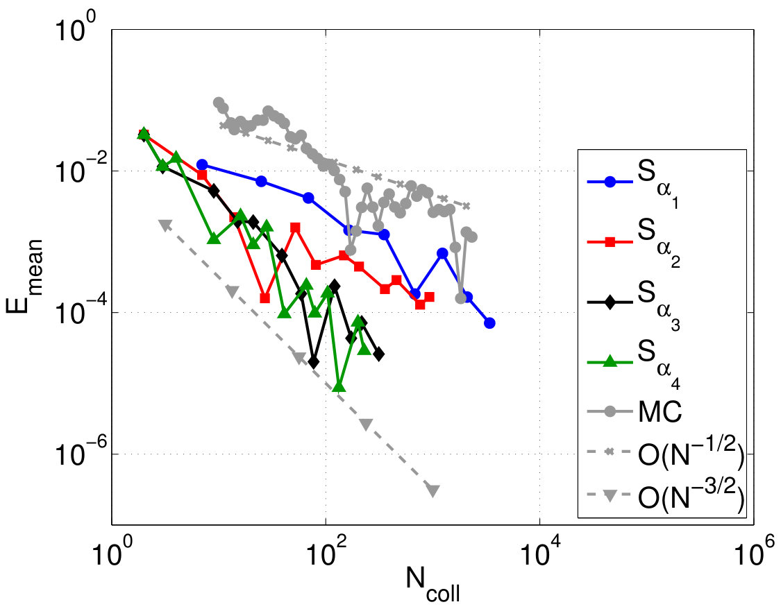 Figure 14
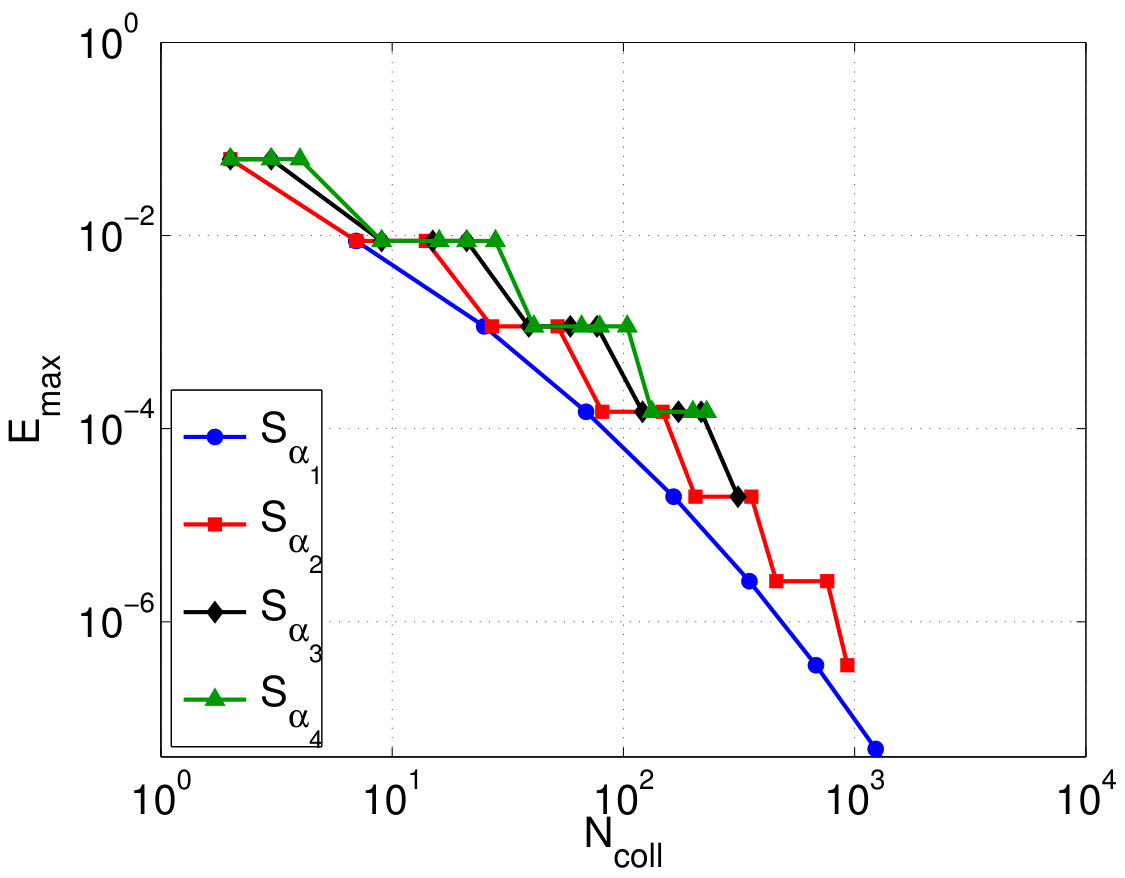 Figure 15
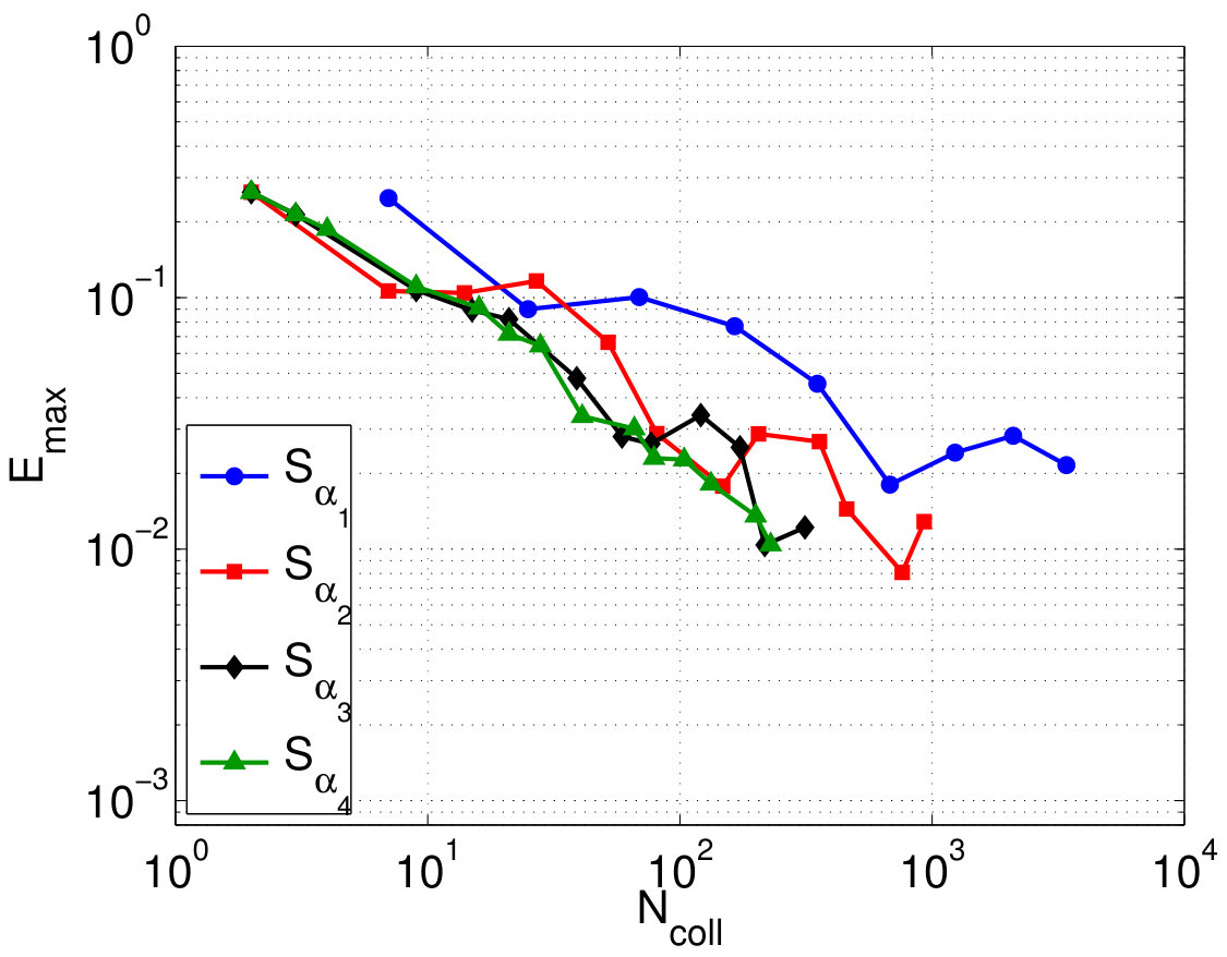 Figure 16
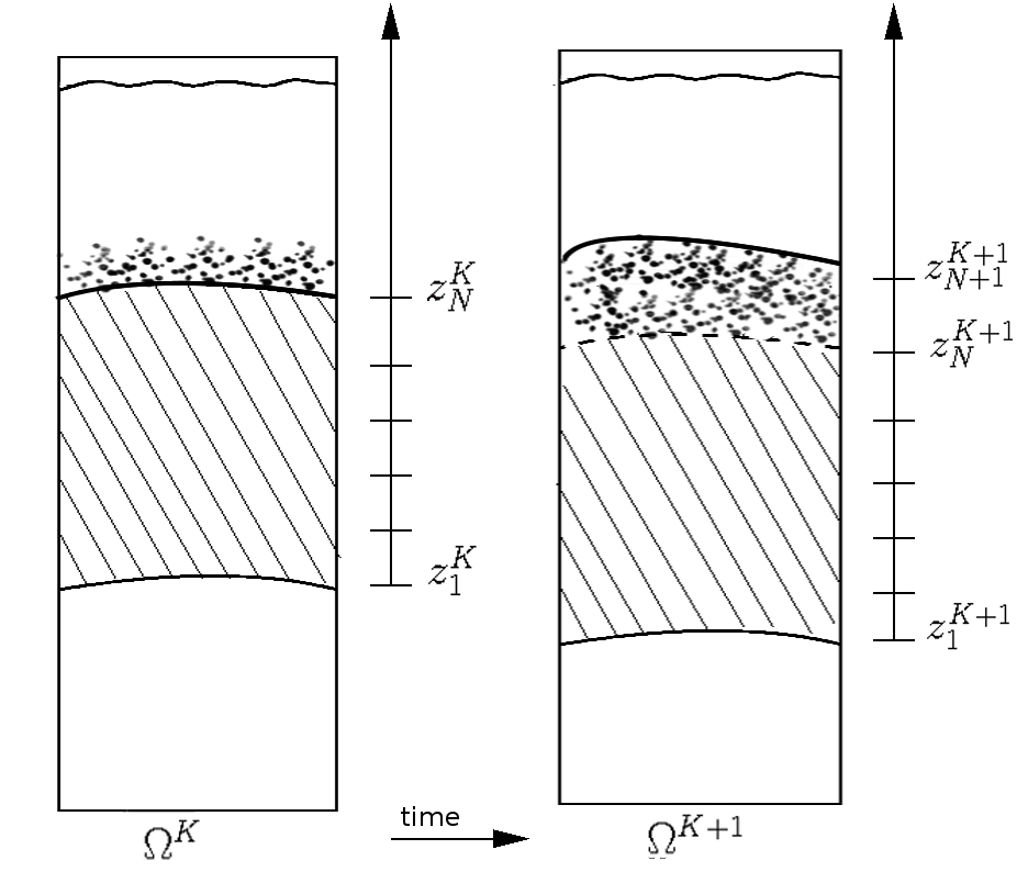 Figure 17
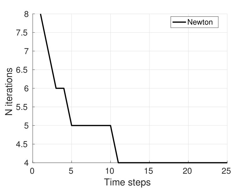 Figure 18
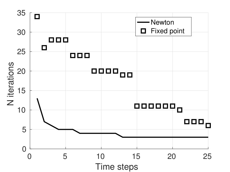 Figure 19
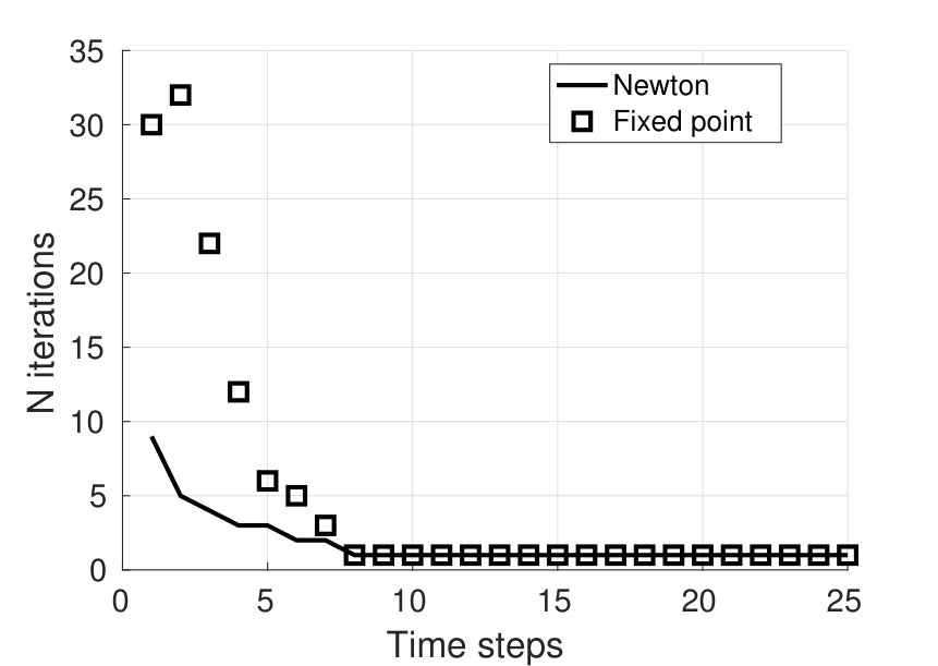 Figure 20
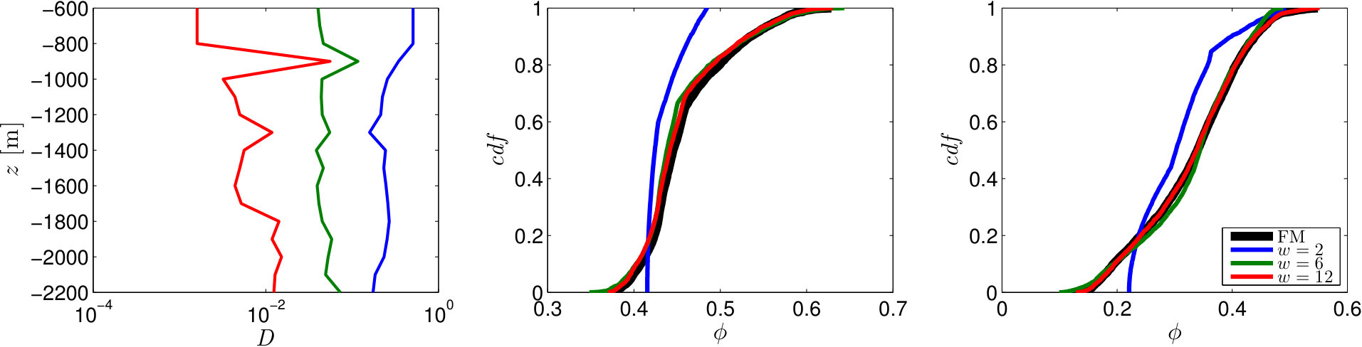 Figure 21
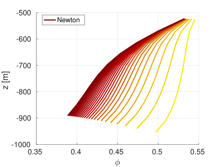 Figure 22
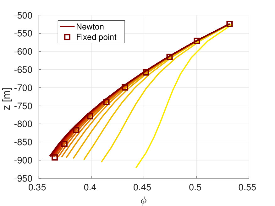 Figure 23
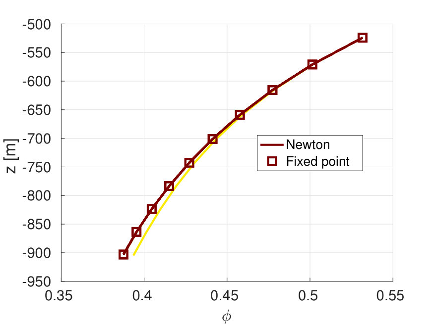 Figure 24
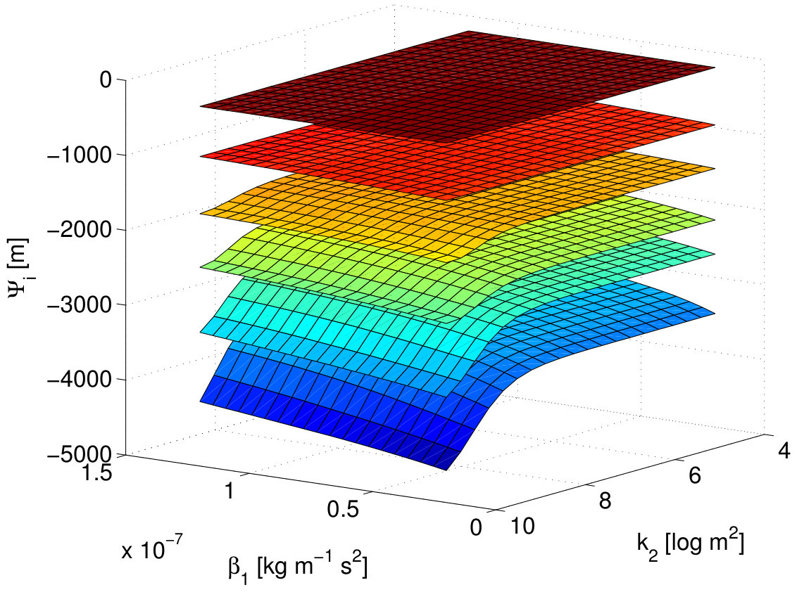 Figure 25
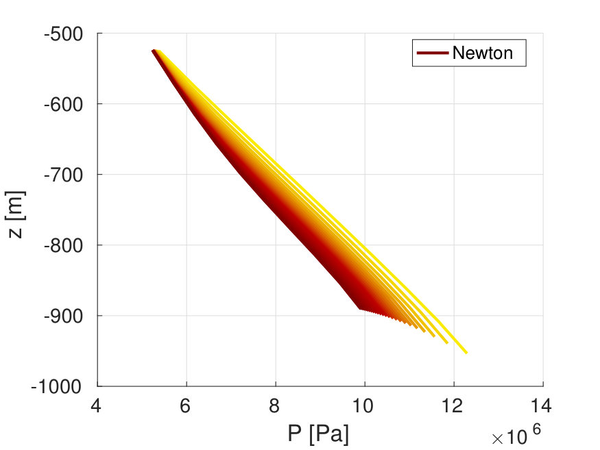 Figure 26
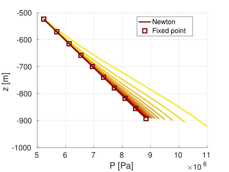 Figure 27
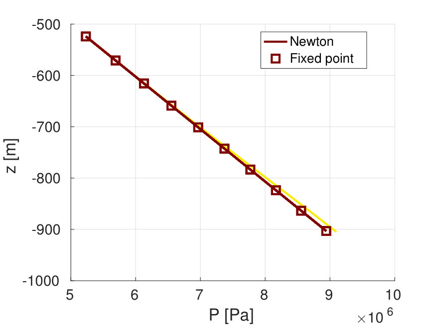 Figure 28
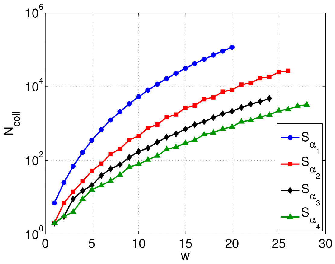 Figure 29
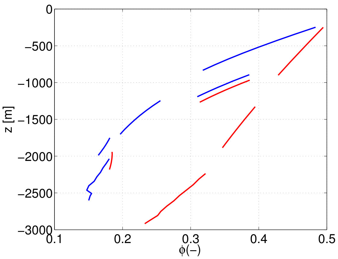 Figure 30
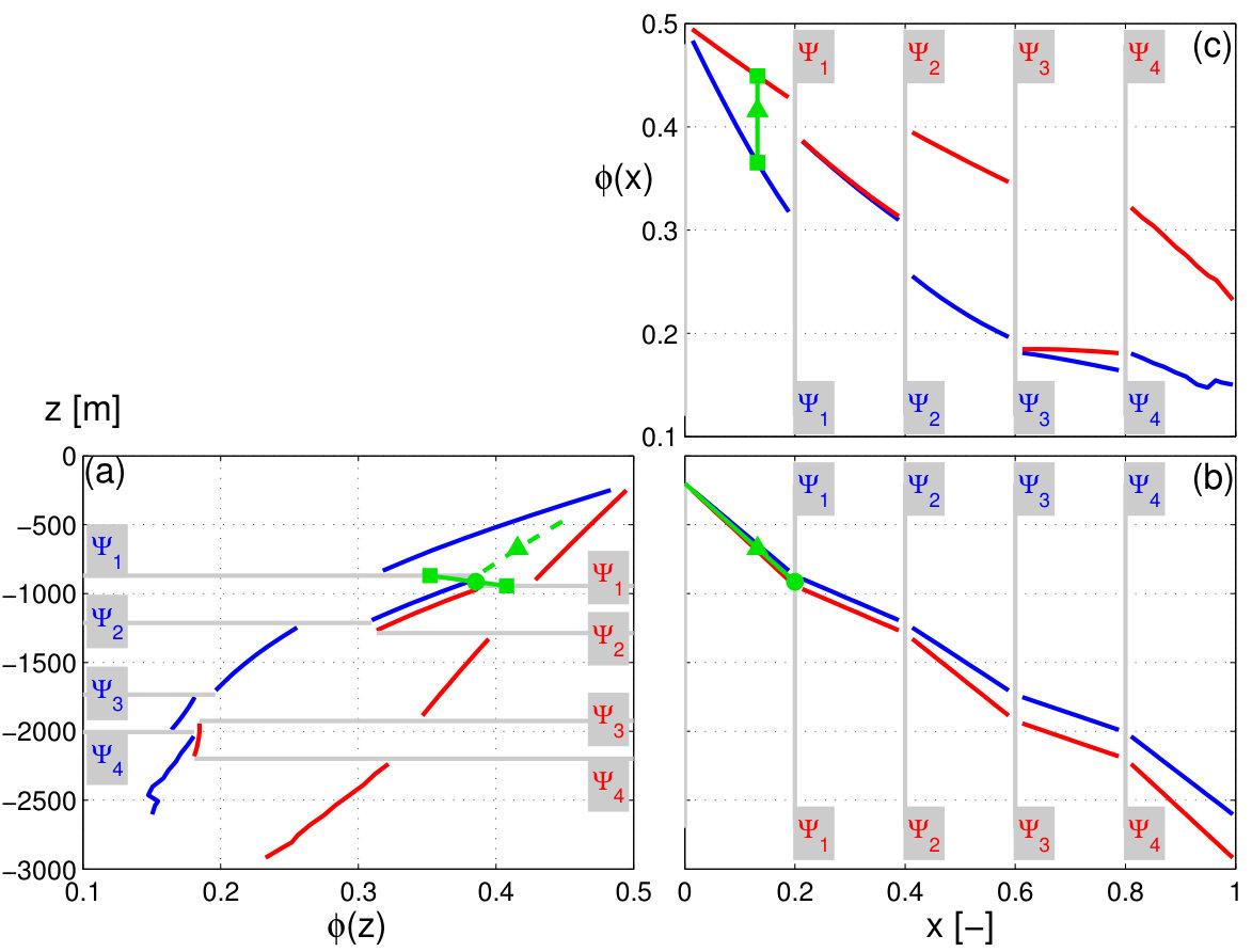 Figure 31
| Initial thickness | 500 | Initial porosity | 0.55 |
|---|---|---|---|
| Sea depth | 500 | Compressibility | 4.0e-7 |
| Rock density | 2648 | Time span | 2.5 |
| physical meaning | symbol | parameter space |
|---|---|---|
| param. for compaction in sandstone | ||
| param. for compaction in shale | ||
| param. of K- law | 4 - 10 |
| SEDIMENTATION CHARACTERISTICS | ||||
| parameter | value | units | ||
| total sedimentation time | 100 | Ma | ||
| constant sedimentation rate | 40 | m | ||
| depositional order (and time) | 1. sand (20) 2. shale (20) 3. sand (20) 4. shale (20) 5. sand (20) | (depositional time [Ma]) | ||
| INITIAL AND BOUNDARY CONDITIONS | ||||
| parameter | value | units | ||
| bathymetric high ( ) | 200 | m | ||
| temperature at basin top ( ) | 295.15 | K | ||
| heat flux at basin basement ( ) | 0.024 | K | ||
| Darcy flux at basin basement ( ) | 0 | m | ||
| FLUID CHARACTERISTICS | ||||
| parameter | value | units | ||
| fresh water density ( ) | 999 | kg | ||
| seawater density ( ) | 1025 | kg | ||
| viscosity ( ) | kg | |||
| specific thermal capacity ( ) | 4186 | J | ||
| specific heat conductivity ( ) | 0.6 | W | ||
| POROUS MEDIUM CHARACTERISTICS | ||||
| parameter | value | units | ||
|
||||
| density ( ) |
|
kg | ||
| specific thermal capacity ( ) |
|
J | ||
| specific heat conductivity ( ) |
|
W | ||
| sediment porosity at deposition ( ) |
|
- | ||
| residual porosity ( ) |
|
- | ||
| , porosity-permeability law |
|
|||
| , porosity-permeability law |
|
|||
| QUARTZ CHARACTERISTICS | ||||
| parameter | value | units | ||
| density ( ) | 2650 | kg | ||
| molar mass ( ) | kg | |||
| initial specific surface area ( ) | ||||
| parameter of reaction model ( ) | mol | |||
| parameter of reaction model ( ) | 0.022 | |||
| activation temperature ( ) | 373.15 | K | ||
Peer Reviews
No public reviews on file for this paper yet. If you reviewed it on a platform where reviews are public (OpenReview, ICLR, NeurIPS, ICML), you can paste yours below so the community can read it here.
Videos
No videos yet. Explain this paper in a talk, walkthrough, or lecture? Add one.
Taxonomy
TopicsProbabilistic and Robust Engineering Design · Reservoir Engineering and Simulation Methods · Advanced Numerical Methods in Computational Mathematics
Uncertainty Quantification of geochemical and mechanical compaction in layered sedimentary basins
Ivo Colombo
Fabio Nobile
Giovanni Porta
Anna Scotti
Lorenzo Tamellini
Dipartimento di Ingegneria Civile e Ambientale, Politecnico di Milano, Piazza Leonardo da Vinci 32, 20133 Milano, Italy
CSQI - MATHICSE, École Polytechnique Fédérale de Lausanne, Station 8, CH 1015, Lausanne, Switzerland
MOX, Dipartimento di Matematica, Politecnico di Milano, Via Bonardi 9, 20133 Milano, Italy
Istituto di Matematica Applicata e Tecnologie Informatiche “E. Magenes” - CNR, Via Ferrata 5, 27100 Pavia, Italy
Abstract
In this work we propose an Uncertainty Quantification methodology for sedimentary basins evolution under mechanical and geochemical compaction processes, which we model as a coupled, time-dependent, non-linear, monodimensional (depth-only) system of PDEs with uncertain parameters. While in previous works (Formaggia et al. 2013, Porta et al., 2014) we assumed a simplified depositional history with only one material, in this work we consider multi-layered basins, in which each layer is characterized by a different material, and hence by different properties. This setting requires several improvements with respect to our earlier works, both concerning the deterministic solver and the stochastic discretization. On the deterministic side, we replace the previous fixed-point iterative solver with a more efficient Newton solver at each step of the time-discretization. On the stochastic side, the multi-layered structure gives rise to discontinuities in the dependence of the state variables on the uncertain parameters, that need an appropriate treatment for surrogate modeling techniques, such as sparse grids, to be effective. We propose an innovative methodology to this end which relies on a change of coordinate system to align the discontinuities of the target function within the random parameter space. The reference coordinate system is built upon exploiting physical features of the problem at hand. We employ the locations of material interfaces, which display a smooth dependence on the random parameters and are therefore amenable to sparse grid polynomial approximations. We showcase the capabilities of our numerical methodologies through two synthetic test cases. In particular, we show that our methodology reproduces with high accuracy multi-modal probability density functions displayed by target state variables (e.g., porosity).
keywords:
Sedimentary basin modeling , Uncertainty Quantification , Random PDEs , Sparse grids , Stochastic Collocation Method
MSC:
[2010] 41A10 , 65C20 , 65N30
1 Introduction
Sedimentary basins occupy depressions of the Earth’s crust where different materials may deposit along geologic times. Numerical simulation of compaction processes in sedimentary basins is relevant to a number of fields, e.g. for the characterization of petroleum systems in terms of hydrocarbon generation and migration [1, 2], understanding of large scale hydrologic behavior (e.g., compaction-driven flow or development of fluid overpressure) [3, 4, 5, 6, 7, 8, 9, 10, 11], or modeling the formation of ore deposits [12].
Modeling basin scale compaction requires to consider mechanical compaction due to the sediments overburden. Moreover, geochemical processes may also occur, due to chemical precipitation and/or dissolution of minerals, and these may heavily affect the effective properties of the system (e.g., porosity, permeability). The mechanics and fluid dynamics of the system evolve as a result of these coupled processes [13, 14]. Key target outputs of basin compaction models are the porosity, pressure and temperature spatial distributions along the basin history.
The geomechanical evolution of subsurface systems and the characterization of fluid dynamics in geological media are classical applications for Uncertainty Quantification methodologies. This can be explained upon considering that our knowledge of geological and physical aspects and of the multi-scale spatial heterogeneity of the subsurface is typically incomplete. In the case of basin compaction we also deal with large characteristic evolutionary scales (millions of years, Ma) and considerable spatial dimensions (km). In this context direct measurements for the characterization of the key processes at the pertinent scale are typically scarce if not lacking altogether, and therefore the boundary conditions and the model parameters are generally poorly constrained. A common approach to deal with this lack of knowledge is to model the uncertain parameters as random variables, and to consider the model predictions as the outputs of a random input-output map, to be analyzed with statistical techniques.
In previous contributions we have developed a forward and inverse modeling technique for basin scale compaction under uncertainty [15, 16], in a simplified framework in which we assume that compaction mainly takes place along the vertical direction. This allows for a relevant simplification of the model structure which is reduced to a one-dimensional (vertical) setting. In this context, our uncertainty quantification technique relies on a sparse grids polynomial surrogate model of the input-output map [17, 18, 19, 20, 21], which approximates the full compaction model outputs (e.g., porosity, temperature or pressure vertical profiles). The sparse grid construction requires first to solve the full compaction model for a number of parameter combinations, which is performed in [15, 16] through a fixed iteration algorithm. The sparse grid approximation can then be algebraically post-processed to obtain relevant information for the Uncertainty Quantification analysis, such as statistical moments and Sobol indices of the quantities of interest. Results by [15, 16] demonstrate that this approach is very effective for the quantification of uncertainty when the basin has sediments with homogeneous properties, as in such a case the key outputs are typically smooth functions of the model parameters.
In this contribution we extend the approach to the case of a multi-layered material. Crucially, in the multi-layer case some state variables experience discontinuities across the different layers, since they typically assume different values depending on the properties associated with the geo-material. For example, the evolution of porosity can considerably change between sandstone and shale units, due to (i) the different mechanical properties associated to the sediments and (ii) geochemical processes leading to porosity changes which selectively take place as a function of the local sediment composition (our model e.g. considers porosity reduction due to quartz cementation which may largely affect porosity only in sandstone layers). The occurrence of such sharp variations across interfaces poses two key issues to the numerical approach proposed in [15, 16].
First, when stratified materials are of concern, permeability contrast of several order of magnitude are commonly found, e.g., across interfaces between permeable sandy layers and shale units characterized by very low permeability. For such low values, the fixed iteration method proposed in [15] is prone to failure. In this work we solve this issue by implementing a Newton iteration algorithm, which considers the fully coupled system of mass, momentum and energy conservation along the basin depth, together with the constitutive relations which are associated with geochemical reactions .
A second key challenge of multi-layered cases is that when multiple model parameters are considered to be random, a single space-time location may be associated with the presence of different geo-materials when different realizations of the random parameters are considered. This results in a discontinuous input-output map and a sparse grid (global) polynomial approximation of it will typically feature a loss of accuracy and fairly low convergence rate.
The occurrence of discontinuities or sharp gradients in input-output maps is rather frequent in mathematical models describing physical problems which are of interest in the context of engineering and applied mechanics, such as conservation laws or advection-dominated transport processes. Special numerical methodologies and procedures have been recently proposed to address this issue in various contexts. Discontinuities in the parameters space have been typically tackled in literature with multi-element approximations [22, 23, 24, 25], multi-wavelet approaches [26, 27, 28], discontinuities-tracking algorithm [29, 30, 31, 32, 33, 34, 35], or by suitably choosing or enriching the polynomial approximation basis [36, 37]. Another possibility is to transform the target variables into proxies which are more amenable to polynomial approximation, see e.g. [38, 39, 40].
We propose here an alternative approach based on the observation that, although the state variables at a fixed depth depend in a discontinuous fashion on the uncertain parameters, the depth of the interfaces among layers actually features a smooth dependence on the parameters and can therefore be accurately approximated by a sparse-grids approach. Upon estimating the interface depth location, we can then map each realization onto a reference domain in which the discontinuities in depth are aligned, and perform a second sparse-grids interpolation in this reference coordinate system, in which the layers never mix and hence sparse grids approximation of the state variables is effective.
While our approach is clearly different from multi-element approximations in the parameter domain, we remark that it is not a discontinuity-tracking algorithm in the parameter space either; in other words, we stress the fact that we do not try to approximate the boundary of the regions of the parameter space that generate porosity profiles (or any other state variables of interest) such that a specific geomaterial will be found at a specific depth. This approach would actually be rather unconvenient and quite challenging in high dimensional parameter spaces, given that such region will in general depend on the depth of interest, therefore we would need to track not one but multiple discontinuities in the parameter space. Instead, for each value of the parameter, we predict the location of the physical discontinuities, that can be accurately predicted by a sparse grid by exploiting the physical properties of our specific problem of interest.
The rest of this work is organized as follows. First, the mathematical model and its deterministic numerical discretization are presented in Section 2. We then describe the methodology employed to deal with discontinuities in the parameters space in Section 3. In particular, we first recall some basics of sparse grid surrogate model construction and then motivate why discontinuities occur and propose a suitable numerical treatment. In Section 4 we showcase the capabilites of our proposed approaches through synthetic test cases, characterized by a realistic evolution. Finally, some conclusions are presented in Section 5.
2 Basin Compaction Model
In this section we provide a description of the mathematical formulation that we employ to model compaction phenomena at sedimentary basin scale and the corresponding numerical discretization strategy adopted. We consider two main drivers for compaction:
Mechanical compaction, acting in the full rock domain and essentially due to the load of overburden sediments, is described as a rearrangement of the deposited grains and the ensuing reduction of porosity. Its effect is considered proportional to the effective stress which is defined as the difference between total stress (lithological pressure) and pore water pressure.
- 2.
Geochemical compaction, acting in the sand-rich materials and related to quartz dissolution and precipitation, provokes reduction of porosity once the mechanism starts: the interstices are increasingly filled with quartz crystals. The minimum values that porosity could reach in this way are significantly lower than those related to pure mechanical compaction.
Following previous approaches [11, 13, 15], we rely on the assumptions that (a) the most relevant phenomena take place mainly along the vertical direction and (b) the rock domain is assumed to be fully saturated by a single fluid characterized by uniform properties. Note that the first assumption enables us to consider a one-dimensional system described by the domain (t) = [(t), (t)], where and denote the bottom and the top of the rock domain respectively, which can both vary with time. These assumptions introduce considerable simplifications with respect to the reality of sedimentary systems, e.g. by overlooking the occurrence of density driven or multi-phase flows. At the same time our simplified approach is still capable of interpreting porosity and pressure distributions observed in real sedimentary systems [11]. In this context a key advantage of introducing a simplified model is that uncertainty propagation can be thoroughly characterized at limited computational cost, a task which would be unaffordable if we were to explicitly model the evolution of a three-dimensional system along geological scales.
2.1 Mathematical model
We describe the time evolution of sedimentary materials along depth through a coupled system of partial differential equations. We impose mass conservation for the solid and fluid phase along the vertical direction by a standard formulation of the conservation laws
[TABLE]
[TABLE]
where [-] is the porosity of sediments; [m ], [kg ] and [kg ] are the velocity, the density and the source term of phase i (where i = s or l, for the solid phase or the fluid phase) respectively. The last term conveys the effect of solid and fluid generation, generally related to geochemical processes.
Displacement of pore water is defined as the difference between the velocity of fluid and solid phase and is described through the equation
[TABLE]
where [m ] is the Darcy flux, [] is the permeability, [kg ] is the fluid dynamic viscosity, [kg ] is the pore pressure, [m ] is the gravitational acceleration.
Following [14] , we set
[TABLE]
where the permeability is given in [] and and are empirical fitting parameters. These two parameters are usually estimated considering experiments at laboratory scale ([14]) or analysis on core data ([41, 8]). Even if this empirical formulation was developed for sandstone and sand-rich material, it is also widely employed for clays and shales [14, 41, 8], upon proper tuning of the values of and . This modeling choice is consistent with published dataset (see, e.g., [8]).
The effect of mechanical compaction is described following the approach of [42]
[TABLE]
where
[TABLE]
is the material derivative. is the material porosity variation due to mechanical compaction, [ m ] is the porous medium (uniaxial) vertical compressibility, is the sediment porosity value at time of deposition, is the minimum porosity value achieved by pure mechanical compaction, and [kg ] is the vertical effective stress, defined as the difference between lithostatic pressure and pore water pressure.
Quartz precipitation is considered modeled following [43]
[TABLE]
[TABLE]
where [-] is the quartz volumetric fraction; [kg ] is the quartz molar mass; [kg ] is the density of quartz; [] and [-] are respectively the specific surface and porosity at the onset of quartz cementation; [mol ] and [] are system parameters. The activation of this reaction is temperature dependent: quartz starts to precipitate when temperature T reaches a critical value that is generally assumed to range from 353 to 373 K ([44]).
As a consequence of equations (5)-(6), the porosity variation is then described by , where and denote the porosity variation due to mechanical compaction and quartz precipitation, respectively.
Temperature evolution inside the rock domain is modeled by
[TABLE]
[TABLE]
[TABLE]
where [kg ] is the effective thermal capacity of the medium, and [ ] are the liquid and solid specific thermal capacities, respectively; [kg m ] is the thermal conductivity; and and are fluid and solid specific conductivities ([14]). Equation (7) includes dynamics of heat exchanges due to fluid advection, solid displacement and thermal diffusion.
An appropriate selection of initial and boundary conditions is needed for the solution of the nonlinear system of partial differential equations (2)-(7). The basement that lies below the sedimentary basin is typically composed of rocks of igneous and metamorphic origin. We assume here that the basement can be considered as an impermeable layer, upon imposing zero fluid flux at . We assume that the considered sedimentary system is submerged below the sea level, to which we assign constant depth , i.e. we set . To take into account the presence of the sea water layer a fixed load proportional to the overlying water depth is assumed on the top of the basin, i.e. . At the top location temperature is also assigned equal to as a Dirichlet boundary condition. A heat flux is assigned as a Neumann boundary condition at the bottom of the basin, by fixing the local vertical derivative .
2.2 Numerical discretization
The numerical discretization follows to a large extent the strategy described in [15] concerning the space and time discretization of the equations, but differs significantly in the non-linear solver.
As in [15] a Lagrangian approach is adopted to address the temporal evolution of the computational domain, i.e. the computational grid is deformed under the effect of compaction according to the solid matrix movement. We have, at each time step , cells and nodes whose position is denoted as for . Due to compaction the size of the elements of the grid, , can change in time. To include the deposition of new sediment layers over time we take into account sedimentation by a modified load at the top of the basin until the thickness of fresh sediments equals the characteristic size of the mesh elements. At that point, a new element is added to the computational grid, see figure 1.
Thanks to the Lagrangian approach it is straightforward to account for the presence of different layers, characterized by different mechanical and chemical properties as required by the applications considered in this study. The evolution equations of the model are discretized in time with the Implicit Euler method. The size of the time step is chosen according to the averege sedimentation rate of the case of interest in such a way that a new cell grid of size is added at the top of the domain after time step:
[TABLE]
Concerning space discretization, mixed finite elements are used for the pressure and temperature problems, in particular pressure and temperature are approximated with piecewise constant elements, while for Darcy velocity and heat flux we employ, since we are considering a 1D domain, simply nodal elements.
For the numerical solution of the resulting system of coupled equations a common approach, used in previous works such as [15], consists in an iterative splitting, i.e. the problem is split into sub-problems that are solved in sequence, possibly iterating until convergence is achieved. However this strategy, in the formulation proposed by [45] and based on an idea first presented in [46], has proven to be unstable for low permeable materials, due to the strong coupling between pressure and porosity.
For this reason, since we are interested in simulations that involve multiple material layers with uncertain parameters we resort to a more robust strategy. In particular, the nonlinear coupling is solved by Newton iterations. We consider the full system of equations which, after discretization in space and time, can be written as
[TABLE]
where are vectors containing the nodal or cell values of the discrete unknowns: the position of the grid nodes , the volumetric fraction of precipitated quartz, the mechanical and effective porosity, the sedimentary load, the fluid pressure and the Darcy velocity.
If we set the iteration of Newton’s method reads
[TABLE]
being the Jacobian matrix of . For each time step the initial guess is given by the solution at the previous time step. The stopping criterion is a simple test on the grid nodes:
[TABLE]
where denotes the size of the cell at the iteration of Newton’s method.
A more stringent test should in principle account for the norm of the vector of the normalized increments. However, due to the different scaling of the variables it is difficult in practice to select an effective tolerance for the whole vector, while a simpler test on the deformation of the domain is robust and representative of the compaction phenomenon.
Note that the position of the st node is given as a boundary condition by the paleobathimetry reconstruction.
Remark**.**
In the present implementation the temperature equation is solved at each Newton iteration separately from the others, after the computation of . This choice is motivated by the fact that temperature is only weakly influenced by the solution of the other equations in the model. However, the nonlinear solver could be easily modified to include the temperature equation.
3 Uncertainty Quantification of the discontinuous outputs of the compaction model
As we have already mentioned, our goal is to extend the previous works [11, 15, 16], to be able to characterize the uncertainty on the quantities of interest computed by the model for multi-layered basins. Throughout this paper, we are only concerned with Uncertainty Quantification for quantities at final time, i.e., today, but the procedure explained in the following applies verbatim to quantities at any intermediate time-step , under minimal assumptions that we will discuss at the end of this section.
Specifically, we suppose that the compaction model has uncertain parameters, which we denote by , and collect them in an -dimensional random vector, . We assume that each uncertain parameter can range in the interval , with , and that each value is equally likely, i.e, we model each as a uniform random variable, with probability density function . The random vector will therefore take values in the -dimensional hyper-rectangle , ; furthermore, it is reasonable to assume that such random variables are independent, therefore the joint probability density function of will be . Denoting by any output of the compaction model at final time today, we are interested in computing quantities such as the expected value and the variance of ,
[TABLE]
or its probability density function .
These operations involve multiple evaluations of for different values of the unknown parameters, and therefore can be very expensive. Thus, a widely used approach to reduce the computational cost of this kind of analysis consists in first building a surrogate model for and then obtaining the quantities detailed above by post-processing. Following the previous works [15, 16] we consider a sophisticated model reduction technique based on a global polynomial surrogate model over the set of parameters, built by a sparse grid approximation formula [17, 18, 19, 20, 21]. However, building an effective sparse grid approximation of state variables such as porosity in the multi-layered case is not straightforward, due to the fact that might actually be discontinuous with respect to , and a dedicated procedure needs to be introduced. In the rest of this section, we briefly recall the stardard sparse grids construction, and then we detail the procedure that we propose to deal with discontinuous response functions. In what follows, let and denote the set of strictly greater than 0 integer and real numbers. Moreover, we will denote by the -th canonical vector of , i.e. a vector with and for for , and by bold numbers, such as and , the vectors of repeated entries .
3.1 Sparse grid approximation
The basic block to construct a sparse grid approximation is a sequence of univariate interpolant polynomials over each (in our case, Lagrange polynomials, as detailed below), indexed by , which thus denotes the univariate interpolation level. For any direction of the parameter space, consider a set of points, , where is a function called “level-to-nodes” function that specifies the number of points to be used at each interpolation level, such that and .
The points should be chosen according to the probability density functions , see e.g. [17]; Gauss–Legendre and Chebyshev/Clenshaw–Curtis points are suitable choices for uniform random variables cf. e.g. [47, 48].
For a fixed level and set of points , we denote by the standard Lagrangian interpolant operator of a continuous function , and furthermore we define the detail operator as
[TABLE]
Observe that building the interpolant (and hence the detail operator) requires evaluating the function at the points of . We also set .
Next, we introduce the multivariate counterparts of and . For any , we write to signify (with a slight abuse of notation) the vector . We begin by letting denote the cartesian grid with points, Upon evaluating any given multivariate continuous function over the points of such grid, we obtain the multivariate tensor Lagrange interpolant of ,
[TABLE]
Note that whenever a component of is zero. Finally, we introduce the so-called hierarchical surplus operators by taking tensor product of details operators,
[TABLE]
The sparse grid approximation of is then defined as a sum of hierarchical surpluses. Namely, we consider a downward closed set111 A downward closed set (also referred to as “lower set”), is a set such that
and define
[TABLE]
where the second equality is known as “combination technique form” of the sparse grid and can be obtained by combining equations (9), (11) and (10) with the first expression in (12), see e.g. [49]. The “combination technique form” can be useful in practical implementations. Observe also that many will be zero: more precisely, if is downward closed then is zero whenever .
The set in (12) prescribes the hierarchical surpluses to be included in the sparse grid, and should be chosen to give good approximation properties while keeping the number of points in the sparse grid to a minimum (remember that one full PDE model solve per point is required to build the sparse grid). Observe that choosing would result in i.e., a multivariate tensor approximation of over a cartesian grid with points along each direction , that is impractical due to the fact that it would require PDE solves. Common choices for are
[TABLE]
and the anistropic counterpart
[TABLE]
where , , are coefficients that are chosen so that a higher polynomial degree is allowed along the directions deemed more important (the more important the random parameter, the smaller the corresponding coefficient ), see e.g. [15, 20, 50]. More advanced strategies for the selection of the set are available in literature: for instance, in [51, 52, 53] an algorithm for optimal sparse grids construction for elliptic PDEs with random coefficients is discussed, while ad adaptive algorithm based on “a-posteriori” refinement has been discussed in [54, 55, 56, 57, 58]. In this work we only discuss results obtained with anisotropic sets of the form (14) (the specific choice of will be detailed later, in Section 4.2). We have also performed some tests with adaptive construction of and obtained analogous results (not shown).
We conclude this introductory section by briefly recalling how relevant Uncertainty Quantification information can be extracted from a sparse grid approximation by suitable post-processing. First, let be the set of collocation points used to build the sparse grid approximation ; one can then associate a sparse grid quadrature formula to , i.e.
[TABLE]
for suitable weights . As a consequence, upon building the sparse grid approximation of , one can immediately compute an approximation of its expected value and higher moments introduced in (8).
Second, by some algebraic manipulations of the combination technique form of the sparse grid approximation , cf. eq. (12), it is possible to compute the so-called Sobol indices of , which quantify which percentage of the total variability of is due to the variability of each random parameter and to their products, in the spirit of a variance decomposition analysis see e.g. [59, 60, 61, 62]. We refer the interested reader to [15, 63] for more details on how to obtain the Sobol indices of starting from its sparse grids approximation ; see also [64].
3.2 Approximation of discontinuous outputs
In this work we focus on sedimentary basins composed by layers of different geomaterials whose interfaces position is random, as it typically depends on the values of the random parameters. As a consequence different kind of geomaterials may be found at a given depth at time for different realizations of the random parameters. This phenomenon is exemplified in Figure 2-left, which shows two vertical distributions of porosity obtained from the direct solution of the mathematical model described in Section 2.1 for two different realizations of the random parameters. The jumps in the porosity profiles are symptoms of geomaterial changes, and it is clearly visible from the figure that interfaces occur at different dephts depending on the random parameter. This implies that the porosity (and other quantities of interest as well) at a fixed depth will be exhibit a discontinuous behavior with respect to the random parameters .
As a consequence, the quality of a standard sparse grid approximation for will be dramatically affected, since sparse grids interpolants are most effective when is a smooth function of the parameters . To circumvent this issue, we propose a methodology that stems from the observation that while quantities at a fixed depth will be likely discontinuous with respect to the parameters , the position of the interface between two materials typically depends smoothly on . This can be observed in Figure 2-right, where we display the variation of the position of the material interfaces as a function of two random parameters, namely the sandstone vertical compressibility and the parameter of the porosity-permeability law (refer to Section 4.2 for more details). This suggests to create a surrogate model for the state variables with a two-steps approach: first, a sparse-grid approximation for the position of each interface is computed, and then the state variables are approximated within each homogeneous lithology.
3.3 A two-steps surrogate model
We detail the procedure referring to the cartoon in Figure 3, which is composed by three panels, (a),(b), and (c), starting from the bottom-left corner and proceeding counter-clock-wise. We focus here on the porosity as an example, but the procedure can be applied verbatim to any other discontinuous output of interest. Figure 3-(a) shows in blue and red two porosity-depth profiles at =today, corresponding to two different realizations of the uncertain parameters, and in green a portion of the porosity profile predicted with our two-steps procedure.
We begin by denoting by the depth of the -th interface as a function of the random parameters, where denotes the seafloor and denotes the bottom of the basin. Note that our procedure assumes that the number of layers does not depend on the random parameters. The seafloor is the upmost interface, i.e., the top of the most recent layer, around (fixed to) m in Figure 3-(a), while the bottom of the basin is the bottom of the oldest layer, whose depth depends on and is around m for the blue profile and around m for the the red profile. As already discussed, the interfaces among geomaterials in the blue and red profiles occur at different depths.
The key idea to create the sparse grid approximations of the state variables is to operate on a layer-by-layer basis, introducing a piecewise linear mapping , that projects the state variables profiles from the physical domain into a reference domain where the discontinuities are aligned, or, in other words, where the interfaces between geomaterials are forced to occur at the same location for every realization of the random parameters. Crucially, since the position of the interfaces is random, the map is random as well, i.e., it depends on . Figure 3 shows two realizations of such map in panel (b) and the aligned porosity profiles in Figure 3(c).
In details, the piecewise linear mapping is defined so that the interfaces are aligned at prescribed values : the seafloor is located at , the bottom of the basin is located at , and intermediate interfaces are located at . Incidentally, note that the reference domain needs not be and could be also e.g , with . Assuming for a moment that are known for a given , then the map can be written as
[TABLE]
In the reference domain, the interfaces are aligned, therefore for a fixed the state variables will always be related to the same layer: therefore, it is reasonable to assume that in the reference domain the state variables at fixed depend smoothly on the parameters, and can be effectively approximated by a sparse grid approximation. In other words, we are implicitely assuming that the behavior of the state variables at any fixed fraction of depth of each layer depends smoothly on the parameters.
Clearly, are not known a-priori; however, the functions can be assumed to be smooth with respect to as we discussed earlier, therefore they can be effectively approximated by sparse grids. Thus, the layer-by-layer state variables approximation algorithm can be summarized as follows:
Construct the sparse grid approximation of the position of the interfaces between layers, for every ; 2. 2.
For every couple of values at which an approximation of is sought (for instance, the location marked by a green triangle in panel (a)):
- (a)
approximate by sparse grids the position of the interfaces for , : in panel (a), the green circle marks the predicted depth at which the first interface will occur, given the location of the first interface for the blue and red profile, marked with squares; 2. (b)
use these values to derive the expression of the piecewise linear mapping and compute : in panel (b), the green circle defines the first portion of the new realization of the piecewise linear mapping, that can be used to compute the reference location corresponding to the physical location of the green triangle in panel (a); 3. (c)
compute the sparse grid approximation of the porosity at , . In panel (c), a green triangle marks the predicted value of porosity at given the porosity values at the same location for the blue and red profile, marked with squares. Observe that some kind of finite element interpolation for the profiles computed with the full model (as the one detailed in Section 2.2) is needed as a preliminary step to compute at the values of porosity that will be used to build ; 4. (d)
approximate .
3.3.1 Discussion on the surrogate model
Before moving to the section showcasing the numerical result, it is worth taking a moment to highlight and discuss features, extensions and possible limitations of the methodology we outlined above.
First, observe that similar approaches to our methodology can be found in [38, 39, 40]. All these works have discussed the advantage that can be obtained by model reduction applied to some ad-hoc transformations of the original output variables designed to improve the accuracy. Our procedure is different in that it is specifically tuned to tackle problems with discontinuities.
Concerning possible extensions, as we have already mentioned, the procedure that we have detailed can be applied verbatim to any time up to today. The only required assumption is that the depositional time of each material be not a random quantity. Indeed, if that was the case, the location of the interfaces would be discontinuous with respect to these random depositional times as well, and this issue would require to be treated analogously to what we propose here for the porosity discontinuities.
We also highlight that the uncertainty quantification methodology proposed here can be extended to the outputs of three-dimensional or two-dimensional models of compaction processes, by applying it pointwise at all locations where uncertainty quantification may be of interest. This can be done under the assumption that the same number of layers is encountered along the vertical direction at all locations. The procedure cannot be applied in its current implementation in the presence of local variations of layering structure which may arise in three-dimensional geological bodies, e.g. in the presence of faults. While we envision dedicated remedies that may be formulated for those specific cases, their discussion is beyond the scope of the present contribution.
Finally, we remark that the choice of the mapping is arbitrary as long as it is globally invertible and smooth within each layer, and thus we have chosen the linear one for convenience. Moreover, our approach rests on the assumption that the limiting factor in the accuracy of the surrogate model is actually the fact that the quantity to be interpolated is discontinuous between interfaces, hence its composition with a piecewise linear mapping does not reduce the overall smoothness.
4 Numerical Results
In this section we illustrate the application of the approach discussed in section 3 to a couple of synthetic test cases. All results reported hereafter have been obtained with Matlab*®* 8.5, using the sparse grids functionalities provided by [65].
4.1 Assessment of the numerical solver for the full model
As we explained in section 2.2 we have chosen, for the solution of the coupled nonlinear system of equations, a monolithic approach with Newton iterations. To prove that this approach is more robust than the iterative splitting proposed in previous works we consider a simple test case and compare the solutions obtained with the strategy proposed in [15] and the Newton method. We consider a single layer that is subject to compaction due to its own weight and a constant overburden . This simple setup avoids inconsistencies due to different initialization of the new cells added to the domain in the two approaches.
The main material and geometric properties are summarized in Table 1.
At the initial time the porosity is uniform and the effective stress is set to zero: then, compaction occurs quickly until the equilibrium configuration is reached. We consider the permeability law (4) and the following values for and :
[TABLE]
with to mimic a variable blend of sandstone and shale. For the sediments are quite permeable and the layer compacts without remarkable overpressure, see figure 4.
As decreases the behavior changes and we observe overpressure counteracting compaction (figure 5). This more complex behavior reflects in a higher number of iterations in particular for the iterative splitting (fixed point) method. Finally for the fixed point method fails to converge while, with the same tolerance and stopping criterion we obtain a solution in 8 iterations with the Newton method. This is due to the complex pressure-porosity interaction, shown in figure 6: in this case, due to the low permeability the iterative splitting of [15] is unstable, while we can always converge to the solution with a fully coupled approach.
4.2 Assessment of the Uncertainty Quantification methodology
We test the procedure described in Section 3 considering a synthetic test case characterized by alternating depositional events of two geomaterials, i.e. sand and shale sediments. Altough most of the effective parameters are affected by considerable uncertainty, given the large space-time scales involved in the compaction processes, here we focus only on those parameters which have the strongest influence on variability of interfaces position. With this idea in mind, we select three uncertain input parameters: and , appearing in Equation (5), i.e. the porous medium vertical compressibility for sandstone and shale, respectively; and the coefficient , which appears in Equation (4) and defines the vertical permeability of shale. The ranges of variability assigned to these materials are listed in Table 2, while Table 3 reports the total sedimentation time, the sedimentation rate and the depositional order of sediments, together with boundary conditions and all other model parameters which are set to fixed values for this analysis.
We consider two cases characterized by two distinct parameter spaces: for case (A) only and are free to vary in selected variability ranges while in case (B) all three parameters are considered uncertain. We consider these two cases to quantify the effect of pure mechanical compaction on interfaces positions against the combined effect of mechanical compaction and vertical fluid flow inside the rock domain. In what follows, we build our sparse grids employing Gauss–Legendre nodes and a linear “level-to-nodes” function, , with index sets (13) or (14). As already mentioned, all results presented hereafter refer to present time.
4.2.1 Approximation of interface positions
Figure 7 displays the distribution of geomaterials (shale and sandstone) obtained upon solving the full compaction model for the collocation points of a sparse grid sampling of the parameter space for the two cases. Each column in the two panels in the Figure represents an independent simulation of the process: the juxtaposition of the results obtained for all collocation points allow to visually appreciate the variability of the interface position as a function of the uncertain parameters (left figure: isotropic sparse grid Equation (13), , 137 collocation points; right figure: anisotropic sparse grid Equation (14), , , 133 collocation points). The results show that interface is constant in all realizations for both cases A and B. This is explained upon observing that the position of this interface is fixed and corresponds to the position of the basin top. Interface also display modest changes as a function of the model parameters for the two considered cases. The remaining interface locations - display variations larger than 100m across the full sample of parameter realizations. We observe however that for case A, for which is fixed to a constant value, the location of interfaces - change by maximum 300m. On the other hand when is considered as uncertain (case B) the location of the deepest interfaces - may vary by up to 1000m across the considered sample.
To identify the impact of each parameter on the variability of the interface position we resort to the total Sobol sensitivity indices , which quantify the contribution of each uncertain parameter to the variance of the interface position (see [15, 16] for an efficient procedure to compute such indices starting from a sparse grid approximation). The results are depicted in Figure 8 for case (A) and (B) respectively. Note that Sobol indices are not computed for the first interface since its position is known and fixed by the boundary condition.
Figure 8-left shows the results obtained for case (A). Its analysis highlights that the position of each interface is sensitive to compaction taking place within materials found at shallower locations than the interface itself. For example, we observe that the position of interface is influenced merely by , sandstone being the only material overlying this interface. The parameter influences the position of to a larger extent than , as this interface is directly underlying a shale lithological unit. For interfaces number , , the influence of the two parameters tends to level off and the difference between and is reduced. These results suggest that for case (A) and have a similar impact on the uncertainty of the position of the interfaces.
Figure 8-right shows the results obtained for case (B). The role of and on the interface position display a similar behavior as in case (A). However, the influence of parameter is predominant on the position of all interfaces with the exception of , which lies beneath the shallowest sandstone unit and therefore does not depend on the parameters governing flow and compaction in the shale layers. For all other interfaces with we obtain . This result indicates that the approximation of the material interfaces may benefit from anisotropic sampling with an increased sampling frequency along the parameter , upon following the criterion in (14).
In the following we refer to case (B) only, which displays larger variations in the interface positions and therefore is more challenging for our uncertainty quantification procedure.
We now aim at assessing the quality of the estimation of the interface positions through sparse grids. To this end, we perform a convergence study of the sparse grid approximation of , measuring the error with the two different error metrics detailed below. Moreover, we will repeat this study for different types of sparse grids, by considering index sets as in (14) with different choices of the vector ; upon fixing the choice of , the convergence study will be done increasing the index sets, hence the number of sparse grid points, by increasing in (14). The relation between the order and the number of sparse grid points, which we denote from here on as , is depicted in Figure 9 for a selected set of sparse grids.
Concerning the choice of , we start from the observation anticipated by the results in Figure 8-right that the position of the interfaces is predominantly influenced by the parameter . Our choice is then to choose such that the resulting sparse grid will be more refined along , while keeping the approximation degree identical along and . To do so, we consider the following four choices for : , , , . Clearly, choosing in (14) is equivalent to building an isotropic sparse grid, i.e. using the set defined in (13), in which all parameters are identically refined. According to the notation introduced above, the grids thus obtained should be denoted by , with ; however, we will employ a lighter notation, i.e. . Similarly, the associated quadrature rules will be denoted by , cf. equation (15).
We employ the following two metrics to evaluate the accuracy of the various sparse grid approximations:
the relative error of the mean position obtained through the sparse approximation
[TABLE]
where identifies the interfaces and is a reference value for the mean of the interface position. We consider here as reference value the mean obtained with a very refined version of the sparse grid , with around 30000 collocation points.
- 2.
the maximum norm of the error of the interface position obtained with respect to the one predicted by the full model simulation within the parameter space
[TABLE]
where is the value of obtained from the direct numerical approximation of the full model. The metric (17) is numerically computed by employing a random sampling of the functions and for . We consider here 1000 random evaluations to compute (17).
Figure 10 displays the two metrics and as a function of the number of realizations required to build each sparse grid approximation. We consider here the variation of the two metrics for the positions and . Note that Figure 10 also reports the results on the convergence of the mean value of and computed by a straightforward Monte Carlo approximation. For interface positions the results are qualitatively similar to those obtained for and for this reason are not reported here.
Results reporting the convergence of interface are reported in Figure 10a-b. A first observation emerges from the comparison between sparse grid and Monte Carlo sampling technique, where the more efficient behavior of the former is highlighted. For example, we find for a number of collocaction points within 60 and 200 depending on the type of sparse grid employed. For the same number of realizations, the mean error associated with the Monte Carlo approach is close to . The position of is approximated with high accuracy by sparse grid surrogate models, with for (see Figure 10a) and (see Figure 10b). Among the sparse grid approximations , are the least effective ones. This can be explained upon observing that only depends on (Figure 8b), so increasing the sampling frequency along adds to the sparse grid points that are not improving the quality of the approximation.
Figure 10c-d displays the results obtained for . For this interface,
the anisotropic sparse grids approximations and still significantly outperform the Monte Carlo approximation, both in terms of error size and convergence rate when metric is considered (Figure 10c) although the improvement is in this case less than for the second interface, due to the increased complexity of the function to approximate, see Figures 2 and 7.
This result shows that anisotropic sampling of the parameter space yields a computational advantage if compared on isotropic one for the approximation of deeply buried interfaces. In the remainder of this section, to test the applicability of the sparse grid technique we select the sparse grid and fix , which yields .
The estimation of the material interface positions allows to estimate the probability to find a specific material at a selected depth in the system. We deal with a conceptual model characterized by alternating deposition of different materials which divide the domain into five macro layers, as listed in the top part of Table 2. The probabilistic distribution of geomaterials along depth can be highly valuable when performing history matching of real sedimentary systems. To obtain this result, we consider now a series of points between m separated by a constant interval of 10m. We then evaluate which material occurs at each of these locations, upon comparing with the estimated interface locations . Note that since depends on the random parameters , then is also random. Figure 11 shows the vertical distribution of probability obtained upon computing the relative frequency , i.e. the probability of observing with . To compute we evaluate the sparse grid approximation over a set of 5000 random points. Figure 11-left shows the vertical distribution of evaluated through the selected sparse grid approximation. Note that for m a single depth is associated with nonzero probability to observe a single material or two materials, close to the interface. For depths deeper than 1700 meters the complexity increases and a single location may be associated with up to three different materials, i.e. , and . These results provide a quantitative assessment of the qualitative observation emerging from Figure 7b.
In Figure 11-right we complement the results in Figure 11-left upon showing the relative frequency of misclassified realizations (), i.e. of realizations for which the value of estimated through the surrogate sparse grid model is different from the one obtained through the direct numerical simulation of the full model for the same parameter combination. The number of misclassified points increases with depth and with the probability to find more than one material at the same depth: in those regions in which the extent of overlapping is small, i.e. between m (i.e. for locations close to ), the frequency is lower than 0.1% while for the deepest locations considered, i.e. for m, the relative frequency of misclassified point increases up a maximum value of 0.8%. This value confirms that the implemented methodology provides a robust estimation of the material interface positions, and can be effectively employed in practice to obtain the probabilistic estimation of the vertical extent associated with all geological units.
4.2.2 Uncertainty quantification for porosity distributions
Finally, we investigate the propagation of uncertainty from input parameters to model outputs considering the probability density functions of porosity at different depths. In order to validate our procedure, the results of the two-step surrogate model procedure are compared against full model results in a Monte Carlo framework. Specifically, we consider a subset of the locations introduced above, we compute for each of them an approximation of the porosity pdf by sampling our sparse grid surrogate model, and we validate the results upon comparing them with those rendered by the full model sampling. As remarked earlier, porosity as a state variable is heavily influenced by the characteristic of the geomaterials.
To assess the accuracy of the results given by the two-step procedure we compare the results in terms of the distance between the cumulative distribution functions (cdfs) of porosity obtained across a range of depths m. This is evaluated as
[TABLE]
where and represent the cdfs of porosity obtained through the numerical solution of the full model or by the two-step model reduction technique introduced in Section 3.3.1, respectively. The left panel of Figure 12 displays the variation of along the vertical direction. The results displayed here are obtained upon approximating and by 5000 Monte Carlo realizations. We consider here various candidate sparse grids surrogate models, which are all obtained from sparse grid approximations upon fixing . We observe that is reduced to values of the order of for , while values typically larger than are attained for . The center and right panels of Figure 12 display the cdfs of porosity for two depths, i.e. at m and m. We select in particular the depth m as it is associated with the largest errors for . We observe that at both investigated depths the sparse grid surrogate associated with approximates the full model response up to a reasonable accuracy, while large errors are observed for . This result is consistent with the observation that the metric (18) is influenced by the accuracy achieved in approximating the location of interfaces, which is discussed above.
We showcase finally the capabilities of our technique upon analyzing in close details the full pdfs of porosity for some specific depth. Since the occurrence of up to three different materials can be observed at some locations, we expect to observe multimodal pdfs of porosity values for those . The pdfs are obtained with Matlab command ksdensity, which is based on a normal kernel function; we have tuned manually the bandwidth of the kernel smoothing window to 0.02, to highlight the multimodality of the pdf.
Figure 13 considers four depths to examine the shape of porosity pdfs obtained with both the sparse grid and the full model solution. In order to sample the vertical domain in a comprehensive way we show here the results associated with four locations, one from the upper part (-600 m), two from the middle (-1350 m, -1500 m) and one from the deepest part of the basin (-2250 m). In addition to the pdfs of porosity we also display for each selected location a scatterplot which allows for a direct comparison between the porosity values predicted with the sparse grid approximation and those given by the full model for the same location and for all considered Monte Carlo realizations of the parameters. In each scatterplot we distinguish the points associated with different materials and we also explicitly tag with red markers the misclassified points introduced above. As a preliminary remark, we observe that the porosity values found for some of the Monte Carlo realizations attain high values (up to 0.8) which are unlikely to be found in a real sedimentary setting (see Figure 13). Here, we detail the results of the full analysis which may be interpreted as a preliminary uncertainty analysis where large uncertainty bounds are assigned to model parameters. In principle, our model reduction methodology allows then to efficiently identify the regions of the parameter space where those values are found and focus on a restricted set of the full parameter space upon excluding unphysical or unrealistic combinations. These may be identified for example from an expected porosity trend which may come from direct field observation or other prior knowledge on the system.
As a first general observation the pdfs yielded by the sparse grid approximation are in close agreement with those obtained through the direct simulation of the full model. Some small differences are only observed for cases where the pdfs shape have a particularly complex and multimodal shape (Figure 13(c)-13(g) ). At m we find material (most recent sandstone layer), for all the Monte Carlo realizations consistently with results in Figure 11. Figure 13(a) and Figure 13(b) show that the values of porosity obtained with the full model and the surrogate basically coincide and span the interval between 0.35 and 0.5. Location m is associated with similar probability of observing material and , see Figure 11a. The shape of the pdf in Figure 13(c) shows three main peaks, which can be tied to the porosity values attained within the two materials which are found at this location across the complete set of realizations of the Monte Carlo sample. This result is therefore informative on the compaction regime which may be observed at this location as a function of the assumed uncertainty of the selected random parameters. In particular we observe that:
The scatterplot in Figure 13(d) puts in evidence that realizations for which material (sandstone) is found at this location tend to cluster around , this value corresponding to the location of a peak of the porosity pdf (see Figure 13(c)).
- 2.
Realizations for which material (shale) is found attain values of porosity of approximately 0.75 (see Figure 13(d)), which correspond to a location of a second peak of the porosity distribution (see Figure 13(c)). These high values of porosity are explained upon observing that the pressure gradient in shale material may become larger than hydrostatic when shale permeability decreases (i.e. as a function of the value assumed by the random parameter ). In these conditions the vertical effective stress decreases and this has a direct effect on porosity through equation (5) (see e.g., [11] for a complete discussion of this phenomenon).
- 3.
a third peak is observed in the porosity pdf for , this value corresponding to the overlap of the porosity distributions in the two materials and . Note that a few misclassified points appear for , i.e. for porosity values which are possibly found in both materials.
At m materials and may be found, with (Figure 11a), i.e. larger probability associated with the presence of (sandstone) than . As a result, the porosity pdf (Figure 13(e)) has here two distinct peaks which are found at porosity values consistent with those observed at depth m, i.e. corresponding to shale material and for sandstone material.
Finally, Figure 13(g) and Figure 13(h) display the results obtained for location m. At this location three different lithological units may be found as a function of the values assumed by the three random parameters across the Monte Carlo sample (see Figure 11a): the largest probability of occurrence is associated with material (shale) followed by (sandstone) and (sandstone). In this case the scatter plot shows a slight increase of the dispersion of the points around the bisector, which indicates that the accuracy of the sparse grid approximation is lower than that observed for shallower locations (compare Figure 13(h) e.g. with 13(b)). The comparison of the pdfs displayed in Figure 13(g) evidences however that these inaccuracies have only a minor consequence on the estimation of the pdf of . Once again, we can tie the observed probability density of to the occurrence of the various geomaterials and relate this to the compaction behavior. The sandstone materials ( and ) tend both to attain smaller porosity values than the shale unit. Note that as the burial depth increases, the maximum observed porosity decreases, i.e. we find here also within shale material .
5 Conclusions
In this paper we devise a methodology for the quantification of uncertainty related to key outputs of sedimentary basins compaction modeling, which considers the evolution along geologic time scales of diagenesis and mechanical compaction phenomena. At these scales, information on the model parameters is typically incomplete and the availability of an uncertainty quantification procedure which is at the same time accurate from a numerical viewpoint and characterized by computational efficiency is of paramount concern. Our methodology embeds reduced order (surrogate) modeling based on sparse grid sampling of a set of unknown parameters, which are considered to be random. Our work leads to the following major results:
We extend here the approach presented in [15, 16] to a case of multi-layered domain, where we have alternating deposition of sand and shale materials. In this case, permeability can attain very low values (typically in shale materials) and exhibit variations of several order of magnitude across layers. In this context the fixed iteration method proposed in previous works ([15]) is prone to failure. We propose here a novel one-dimensional solver grounded on a Newton iteration algorithm for the solution of the fully coupled system consisting of mass, momentum and energy conservation equations, together with geochemical constitutive relations along the vertical direction. The Newton iteration algorithm clearly outperforms fixed point iterations for permeabilities within the range of those typically associated with shale-rich materials. 2. 2.
Specific variables of the problem exhibit sharp variations moving along the vertical direction, which are located at the interface between different geomaterials. The location of such discontinuities is typically function of model parameters. The accuracy of polynomial approximations obtained from standard sparse grid methods typically deteriorates in the presence of discontinuous mapping between input parameters and output variables. We present an original approach to tackle this issue which relies on the assumption that the depth of the interfaces among layers shows a smooth dependence on the parameters and can therefore be accurately estimated with a sparse-grids approach. We consider a synthetic test case characterized by realistic evolutionary scales. Mechanical compaction modulus and shale permeability are considered as random parameters. Sobol’ indices analysis indicates that vertical shale permeability has larger effect than vertical compaction modulus on the location of material interfaces where discontinuities of state variables (e.g., porosity) may occur. 3. 3.
We analyze the convergence of the approximation of the interface locations obtained through sparse grid sampling, based on the mean estimated location of the interfaces and on the maximum error with respect to the full model simulation within the considered random parameter space. We observe that for shallow depths the sparse grid approximation converges rapidly when increasing the number of collocation points, independently of the strategy adopted for the sparse grid sampling approach. For deep locations the input/output mapping becomes more complex. In such conditions, the efficiency of the sparse grid approximation greatly improves when anisotropic sampling is performed, i.e. when the order of the sparse grid approximation increases proportionally to the intensity of the Sobol’ sensitivity indices associated with each parameter. The number of collocation points required to obtain a given level of accuracy may be reduced by two orders of magnitude when considering an anisotropic sparse grid instead of an isotropic one. 4. 4.
We finally investigate the uncertainty propagation from input parameters to model responses which exhibit a discontinuous behavior in the parameter space, i.e. porosity, considering its probability density function at selected depths. We compare the results obtained with the two-step surrogate model and the full model within a Monte Carlo framework. Results indicate that the pdfs associated with the sparse grid approximation are in close agreement with those obtained with the direct simulation of the full model. We display for each selected location also a scatterplot which allows a direct comparison between the porosity values predicted with the sparse grid approximation against those given by the full model for the same location and for all considered Monte Carlo realizations of the parameters. What emerges is that even though for deeper layers the accuracy of sparse grid approximation decrease, points in the scatter plot exhibit an increasing dispersion around the bisector and the number of mismatched points increase, the entity of these inaccuracies is small enough to have only a minor consequence on the estimation of the pdf of porosity. This result suggests that the proposed methodology is suitable to be embedded within model calibration techniques, which will be considered in future works.
Acknowledgement
F. Nobile and L. Tamellini received support from the Center for ADvanced MOdeling Science (CADMOS). L. Tamellini also received support from the Gruppo Nazionale Calcolo Scientifico - Istituto Nazionale di Alta Matematica “Francesco Severi” (GNCS-INDAM).
The reference list from the paper itself. Each links out to its DOI / PubMed record.
- 1[1] K. Tuncay, P. Ortoleva, Quantitative basin modeling: present state and future developments towards predictability, Geofluids 4 (2004) 23–39.
- 2[2] T. Taylor, M. Giles, L. Hathon, T. Diggs, N. Braunsdorf, G. Birbiglia, M. Kittridge, C. Macaulay, I. Espejo, Sandstone diagenesis and reservoir quality prediction: models, myths, and reality, AAPG Bull 94 (2010) 1093–1132.
- 3[3] U. Mello, G. Karner, R. Anderson, A physical explanation for the positioning of the depth to top of overpressure in shale-dominated sequences in the gulf coast basin, united states, Journal of Geophysical Resources 99 (1994) 2775–2789.
- 4[4] J. Hunt, J. Whelan, L. Eglinton, L. Cathles, Relation of shale porosities, gas generation, and compaction to deep overpressures in the u. s. gulf coast: abnormal pressures in hydrocarbon environments, AAPG Memoir 70 (1998) 87–104.
- 5[5] J. Jiao, C. Zheng, Abnormal fluid pressures caused by deposition and erosion of sedimentary basins, Journal of Hydrology 204 (1998) 124–137.
- 6[6] M. Osborne, R. Swarbrick, Diagenesis in north sea HPHT clastic reservoirs consequences for porosity and overpressure prediction, Marine and Petroleum Geology 16 (1999) 337–353.
- 7[7] B. Mc Pherson, J. Bredehoeft, Overpressures in the uinta basin, utah: analysis using a three-dimensional basin evolution model, Water Resources Research 37(4) (2001) 857–871.
- 8[8] C. Neuzil, How permeable are shales?, Water Resources Research 30 (1994) 145–150.