Global and Brazilian carbon response to El Ni\~{n}o Modoki 2011-2010
K. W. Bowman, J. Liu, A. A. Bloom, N. C. Parazoo, M. Lee, Z. Jiang, D., Menemenlis, M. M. Gierach, G. J. Collatz, K. R. Gurney, D. Wunch

TL;DR
This study uses satellite data and carbon cycle models to quantify the global and Brazilian carbon flux responses to the 2010 El Niño Modoki, revealing complex regional contributions and near-zero net ecosystem change in Brazil.
Contribution
It introduces a satellite-based, 4D-variational assimilation approach to quantify spatially resolved carbon fluxes during climate events, specifically applied to the 2010 El Niño Modoki.
Findings
Global net carbon flux tendency was -1.60 PgC (2011-2010).
Brazil's net flux tendency was -0.24 ± 0.11 PgC.
Brazil's biomass burning tendency was -0.24 ± 0.036 PgC.
Abstract
The El Ni\~{n}o Modoki in 2010 lead to historic droughts in Brazil. We quantify the global and Brazilian carbon response to this event using the NASA Carbon Monitoring System Flux (CMS-Flux) framework. Satellite observations of CO, CO, and solar induced fluorescence (SIF) are ingested into a 4D-variational assimilation system driven by carbon cycle models to infer spatially resolved carbon fluxes including net ecosystem exchange, biomass burning, and gross primary productivity (GPP). The global net carbon flux tendency, which is the flux difference 2011-2010 and is positive for net fluxes into the atmosphere, was estimated to be -1.60 PgC between 2011-2010 while the Brazilian tendency was -0.24 0.11 PgC. This estimate is broadly within the uncertainty of previous aircraft based estimates restricted to the Amazonian basin. The biomass burning tendency in Brazil was -0.24 …
Click any figure to enlarge with its caption.
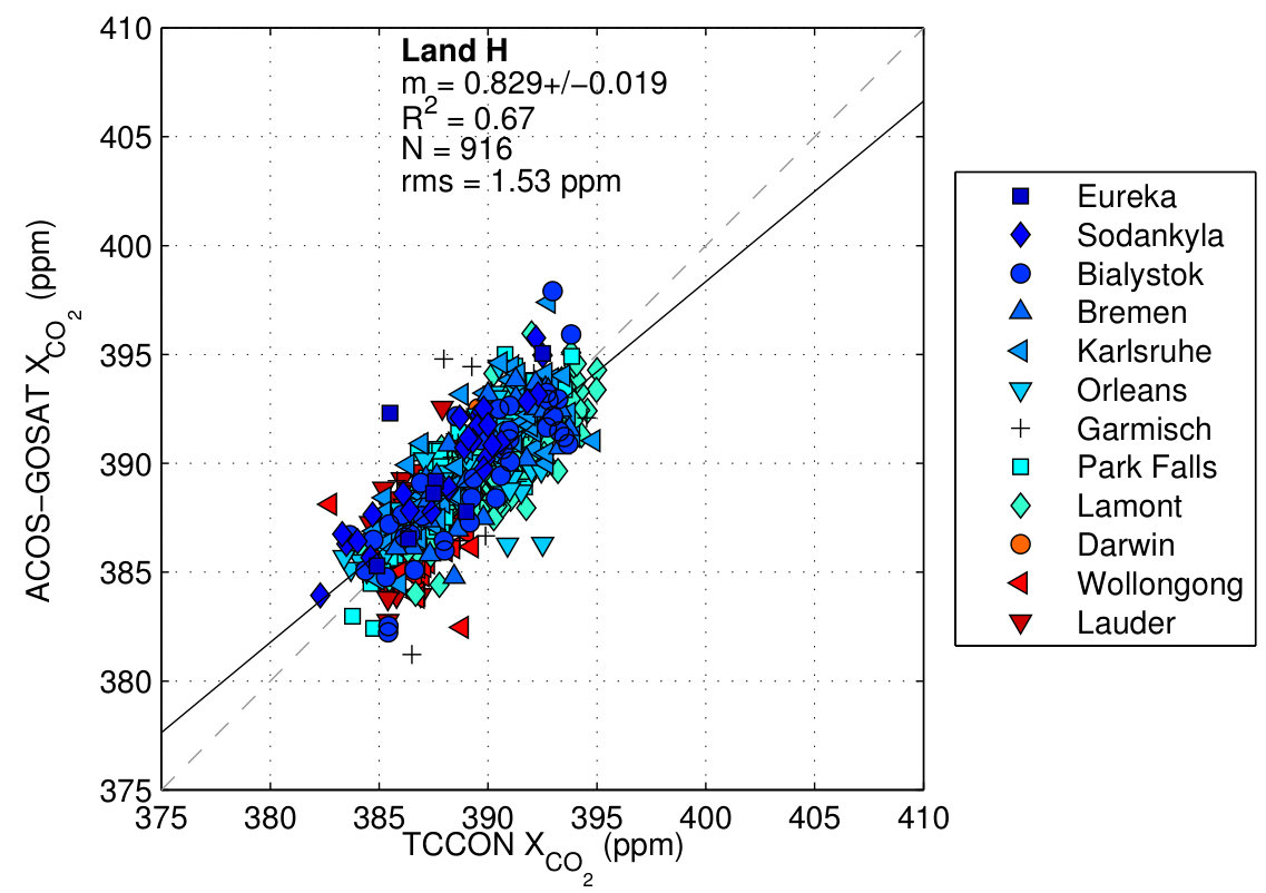 Figure 1
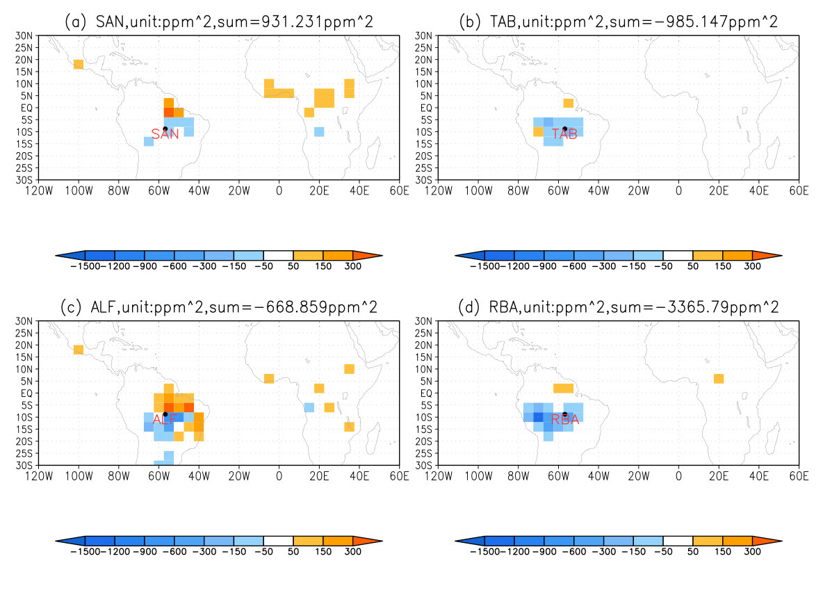 Figure 3
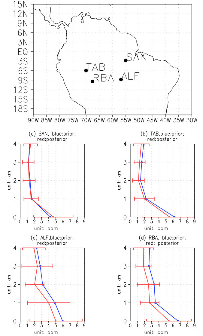 Figure 3
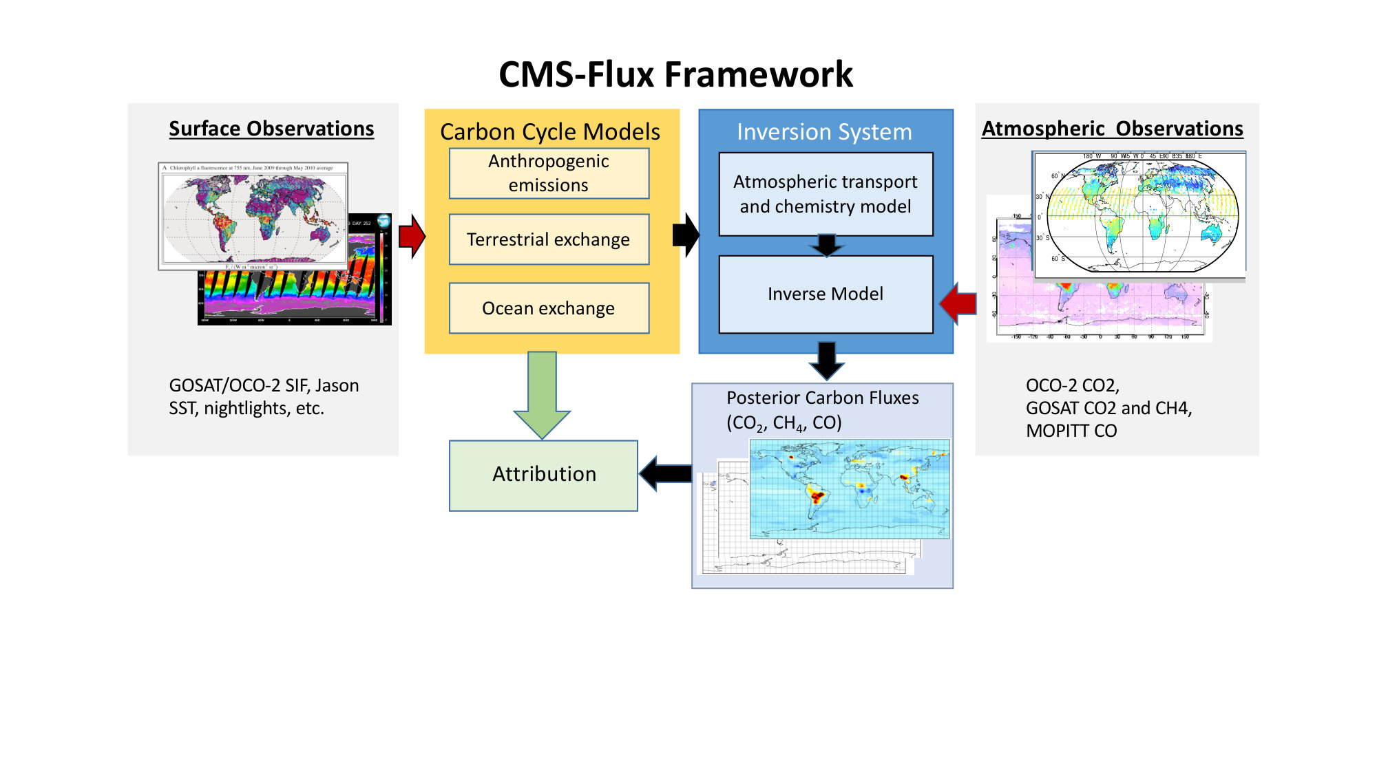 Figure 4
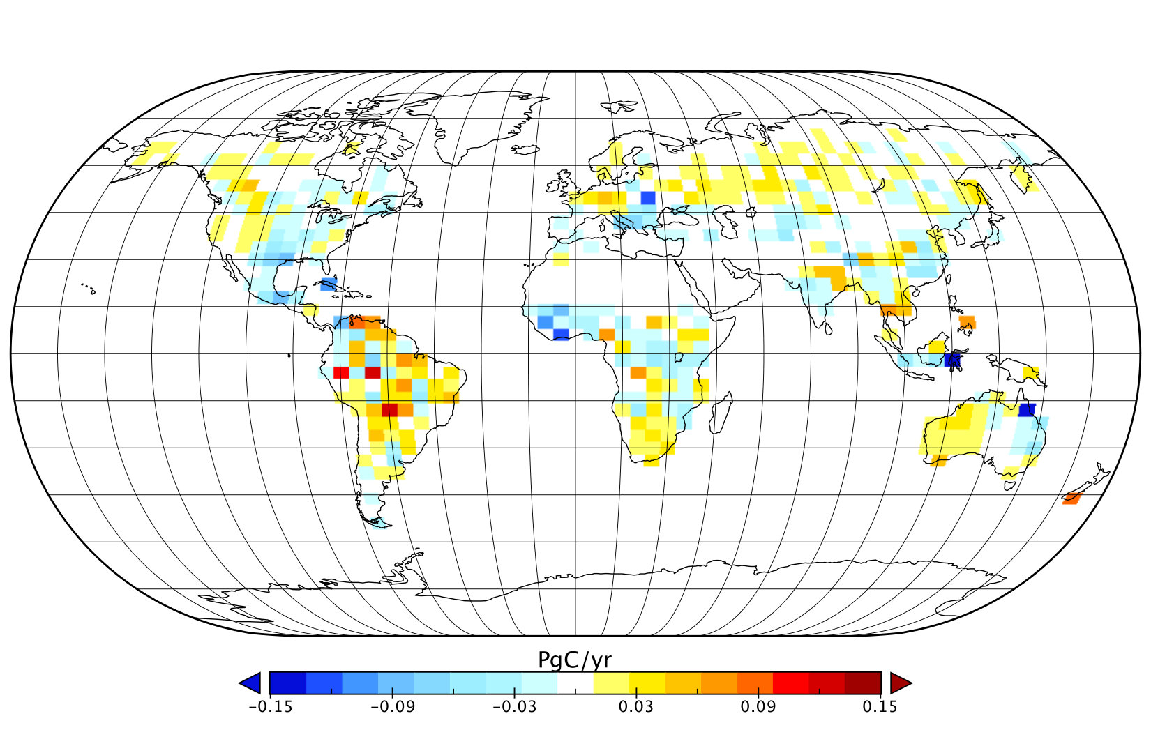 Figure 5
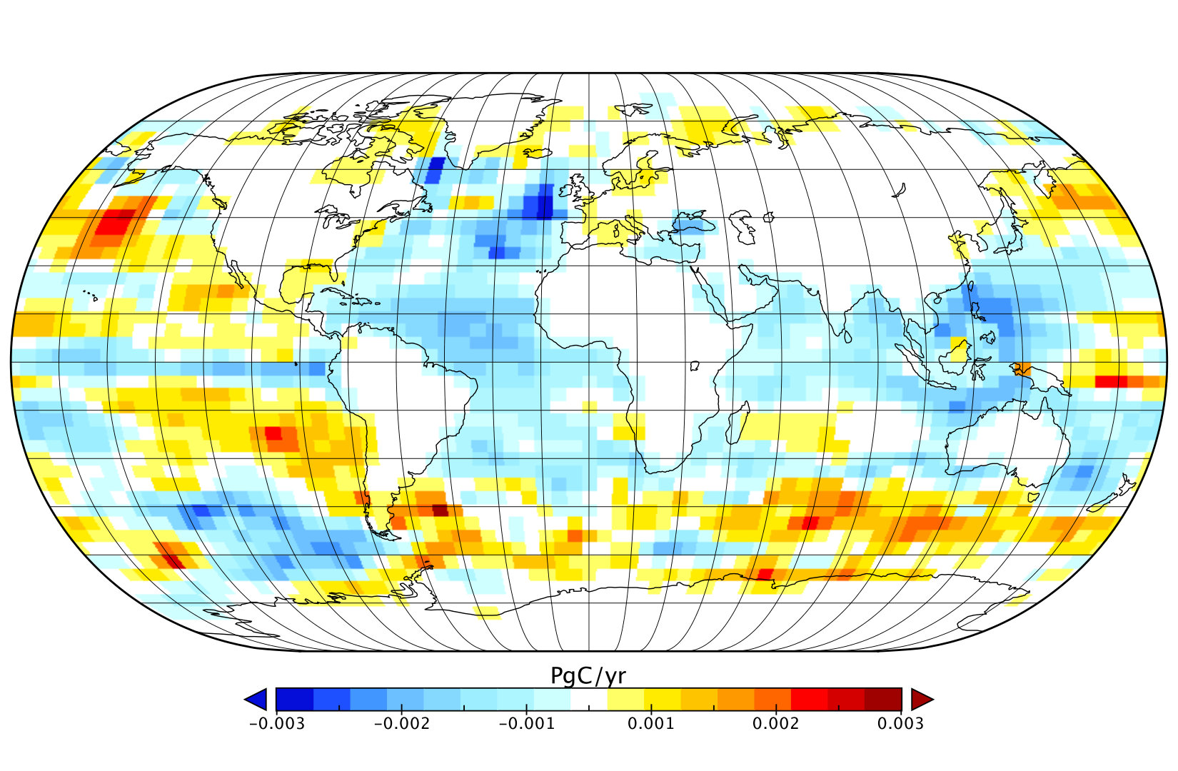 Figure 6
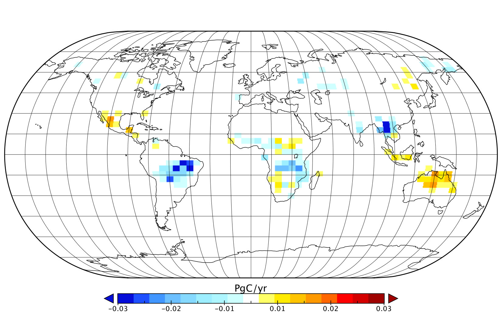 Figure 7
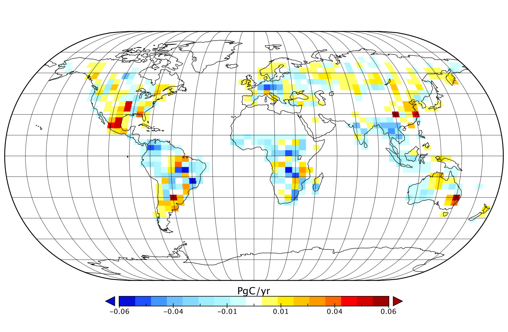 Figure 8
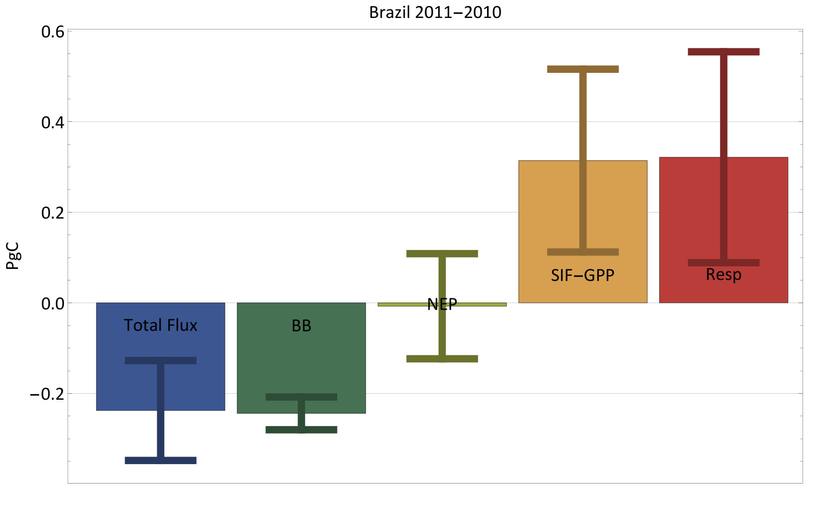 Figure 9
| 2010 | 2011 | |||
|---|---|---|---|---|
| Region | Prior | Post | Prior | Post |
| 15N–90N | -0.24 | 0.03 | -0.11 | 0.08 |
| 15S–15N | 0.34 | 0.31 | 0.42 | 0.26 |
| 15S–90S | -0.59 | -0.16 | -0.69 | -0.10 |
| Year | 2010 | 2011 | uncertainty |
| Growth rate (ppm) | 2.34 | 1.84 | 0.11 |
| Fossil Fuel (PgC) | 9.25 | 9.50 | 0.5 |
| Ocean (PgC) | 2.38 | 2.71 | 0.5 |
| Fire (PgC) | 2.92 | 2.24 | ? |
| Terrestrial (PgC) | 4.85 | 5.79 | 1 |
| Sector | Uncertainty Source | ||||
|---|---|---|---|---|---|
| Ag Waste EF | 92 (94) | 1308 (1452) | 84 | 177 | [Andreae and Merlet (2001)] |
| Deforestation EF | 101 (101) | 1626 (1626) | 24 | 40 | [Akagi et al. (2011)] |
| Extratropical Forest EF | 106 (106) | 1572 (1572) | 44 | 98 | [Akagi et al. (2011)] |
| Peat EF | 210 (210) | 1703 (1563) | 60 | 65 | [Akagi et al. (2011)] |
| Savanna EF | 62 (61) | 1650 (1646) | 17 | 63 | [Akagi et al. (2011)] |
| Woodland EF | 82 (81) | 1638 (1703) | 32 | 71 | [Akagi et al. (2011)] |
| Atlantic | Pacific | Indian | Southern | |
| PgC | -0.187 | -0.008 | 0.011 | 0.017 |
Peer Reviews
No public reviews on file for this paper yet. If you reviewed it on a platform where reviews are public (OpenReview, ICLR, NeurIPS, ICML), you can paste yours below so the community can read it here.
Videos
No videos yet. Explain this paper in a talk, walkthrough, or lecture? Add one.
Global and Brazilian carbon response to El Niño Modoki 2011-2010
Abstract
The El Niño Modoki in 2010 lead to historic droughts in Brazil. We quantify the global and Brazilian carbon response to this event using the NASA Carbon Monitoring System Flux (CMS-Flux) framework. Satellite observations of CO2, CO, and solar induced fluorescence (SIF) are ingested into a 4D-variational assimilation system driven by carbon cycle models to infer spatially resolved carbon fluxes including net ecosystem exchange, biomass burning, and gross primary productivity (GPP). The global net carbon flux tendency, which is the flux difference 2011-2010 and is positive for net fluxes into the atmosphere, was estimated to be -1.60 PgC between 2011-2010 while the Brazilian tendency was -0.24 0.11 PgC. This estimate is broadly within the uncertainty of previous aircraft based estimates restricted to the Amazonian basin. The biomass burning tendency in Brazil was -0.24 0.036 PgC, which implies a near-zero change of the net ecosystem production (NEP). The near-zero change of the NEP is the result of quantitatively comparable increase in GPP (0.34 0.20) and respiration in Brazil. Comparisons of the component fluxes in Brazil to the global fluxes show a complex balance between regional contributions to individual carbon fluxes such as biomass burning, and their net contribution to the global carbon balance, e.g., the Brazilian biomass burning tendency is a significant contributor to the global biomass burning tendency but the Brazilian net flux tendency is not a dominant contributor to the global tendency. These results show the potential of multiple satellite observations to help quantify the spatially resolved response of productivity and respiration fluxes to climate variability.
\authorrunninghead
BOWMAN ET AL. \titlerunningheadBRAZILIAN CARBON BALANCE ©2016 All Rights Reserved \authoraddrCorresponding author: K.W. Bowman, Jet Propulsion Laboratory, California Institute of Technology Pasadena, CA, 91109, USA. ([email protected])
11affiliationtext: Jet Propulsion Laboratory, California Institute of Technology, Pasadena, CA22affiliationtext: Joint Institute for Regional Earth System Science and Engineer, University of California Los Angeles, CA33affiliationtext: NASA Goddard Space Flight Center, Greenbelt, MD44affiliationtext: Ecology Evolution and Environmental Science, Arizona State University, Tempe, AZ55affiliationtext: National Center for Atmospheric Research, Boulder, CO66affiliationtext: Department of Physics, University of Toronto, Toronto
\keypoints
2010 El Niño led to significant droughts in Brazil
Biomass burning from Brazil dominated global biomass burning tendency (2011-2010)
Brazilian net flux tendency -0.24 0.11 PgC is mostly driven by biomass burning
Positive Brazilian GPP tendency observed from solar induced fluorescence measurements is balanced by respiration.
{article}
1 Introduction
In 2011, carbon dioxide (CO2) measurements reached 391 ppm, which is about 40% higher than preindustrial levels. This level substantially exceeds the highest concentrations recorded in ice cores during the past 800,000 years (Stocker et al., 2013). These dramatic changes have led to a planetary radiative imbalance estimated at 0.58 0.15 Wm*-2* from 2005-2010 at the top-of-the-atmosphere (Hansen et al., 2011). Changes in atmospheric temperature, hydrology, sea ice, and sea levels are attributed to climate forcing agents dominated by CO2 (Santer et al., 2013; Stocker et al., 2013). While increases in atmospheric CO2 are a result of fossil fuel emissions, about 55% is removed through terrestrial and oceanic physical and biogeochemical processes (Gloor et al., 2010). The “airborne fraction” (AF) is the ratio of the observed atmospheric CO2 to the CO2 emitted from anthropogenic emissions. While this trend in the airborne fraction has been remarkably stable, some studies have suggested the AF is changing while others dispute this conclusion (Canadell et al., 2007; Knorr, 2009; Le Quere et al., 2009; Gloor et al., 2010). Nevertheless, the majority of carbon-climate models indicate that the AF will likely change in the future as a result of carbon-climate feedbacks (Jones et al., 2013). Assessing these trends is challenging in part due to the significant interannual variability of the atmospheric growth rate linked to natural variability in the climate system (Langenfelds et al., 2002; Wang et al., 2013). Wang et al. (2013) showed that a 1*∘C tropical temperature anomaly leads to a 3.5 0.6 PgC yr-1* CO2 growth rate anomaly (1959-2011) (). Cox et al. (2013) used this same relationship between tropical temperatures and CO2 to apply an emergent linear constraint on the carbon-climate feedback factor–the so-called parameter (GtC K*-1*)–diagnosed from the C4MIP Earth System Models (ESM).
These studies, however, do not pinpoint the spatial drivers of the CO2 atmospheric growth rate. Resolving the source of atmospheric growth rate variability is an important step in assessing the underlying processes driving these changes. Globally distributed atmospheric observations of CO2 have played an important role in quantifying the spatial distribution of CO2 fluxes, (e.g., Rayner et al., 1996; Gurney et al., 2002; Peters et al., 2007; Chevallier et al., 2010, 2011; Ciais et al., 2010; Peylin et al., 2013). One of the fundamental challenges of these approaches to quantify CO2 fluxes has been the sparsity of the surface observations, especially in South America and Africa (Patra et al., 2003). Observations of CO2 from meteorological and atmospheric composition sounders have good coverage over these areas. However, they are primarily sensitive to free tropospheric CO2, which is well-mixed, and consequently has been challenging to use (Chevallier et al., 2005; Engelen et al., 2004, 2009; Nassar et al., 2011). More recently, near-infrared (NIR) observations of column CO2 from the Japanese GOSAT satellite have the potential to greatly improve our understanding regional carbon fluxes (Chevallier et al., 2007; Baker et al., 2010; Hungershoefer et al., 2010). GOSAT has been used to assess CO2 variability in northern and southern latitudes (Guerlet et al., 2013; Wunch et al., 2013; Parazoo et al., 2013), and to quantify CO2 fluxes from megacities (Kort et al., 2012; Silva et al., 2013) and biomass burning (Ross et al., 2013). More recently, GOSAT observations have been used to infer global surface CO2 fluxes (e.g., Basu et al., 2013; Maksyutov et al., 2013; Houweling et al., 2015; Deng et al., 2014, 2016).
We will focus on how the historic 2010 El Niño Modoki and the following La Niña impacted global fluxes generally and Brazilian fluxes in particular. These years provide a useful–though limited–contrast in the changes in atmospheric CO2 growth rate. The atmospheric growth rate observed from the NOAA Mauna Loa site for 2010 was 2.36 ppm yr*-1* in contrast to 1.88 ppm yr*-1* for 2011. The detrended CO2 growth rate anomaly relative to the 1959-2011 mean was 0.7 and -0.3 PgC yr*-1* in 2010 and 2011, respectively. A critical regional climate pattern was a historic sea surface temperature (SST) anomaly in the tropical North Atlantic during 2010 that reached almost 1∘C, breaking the previous record in 2005. This SST anomaly was partly a response to a strong central Pacific or El Niño Modoki, which is associated with strong anomalous warming in the central tropical Pacific and cooling in the eastern and western tropical Pacific, where the El Niño Modoki index exceeded 1.0*∘*C (Ashok et al., 2007; Ashok and Yamagata, 2009). This El Niño Modoki was the largest relative to the previous three decades (Lee and McPhaden, 2010). Hu et al. (2011) showed the anomalous warming was additionally coupled to a strong and persistent negative phase of the North Atlantic Oscillation (NAO). As a consequence, the Intertropical Convergence Zone (ITCZ) shifted north resulting in historic droughts in the Amazon in 2010 (Lewis et al., 2011).
We will use the NASA Carbon Monitoring System Flux (CMS-Flux), which integrates satellite observations across the carbon cycle, to investigate the spatial drivers of these changes and attribute them to regional carbon cycle processes (Liu et al., 2014). Atmospheric observations include xCO2 from the GOSAT instrument, which will be described in Sec. 2 and CO from MOPITT, which will be discussed in Sec. 3. These data along with satellite observations of the land-surface are ingested into the CMS-Flux framework , which is described in Sec. 4. The 4D-variational system used to infer global CO2 and CO fluxes is described in Sec. 4.5. The net CO2 flux is the sum of gross fluxes including biomass burning, gross primary productivity, total ecosystem respiration, fossil fuel, etc. We develop an attribution strategy discussed in Sec. 5 that uses a combination of observations, e.g., solar-induced fluorescence measurements, to estimate individual fluxes and then infer unmeasured respiration fluxes as a residual term. We quantify the global flux tendencies, i.e., the change in flux between 2011 and 2010, derived from CMS-Flux in Sec. 6.1 and then apply this attribution strategy to assess the Brazilian carbon tendency in Sec. 6.2. The limitations and potential of this approach for understanding the role of the El Niño Southern Oscillation (ENSO) on the interannual variability of CO2 will be discussed in Sec. 7.
2 GOSAT satellite
The Japan Aerospace Exploration Agency (JAXA) Greenhouse gases Observing Satellite “IBUKI” (GOSAT) satellite was launched in January 2009. GOSAT is in a sun-synchronous orbit at a 666 km altitude and a 98*∘* inclination with a 12:49 p.m. nodal crossing time and a three-day (44-orbit) ground track repeat cycle (Hamazaki et al., 2005). GOSAT measures both along track () and cross-track () with an instantaneous field-of-view (IFOV) of 10.5 km. The 5-point cross-track scan mode was used between 4 April 2009 and 31 July 2010 providing observations separated by 158 km cross-track and 152 km along track. Afterwards, the mode was changed to 3-point leading to 263 km cross-track and 283 km along-track (M.Nakajima et al., 2010; Crisp et al., 2012). This satellite includes the Thermal And Near-infrared Sensor for carbon Observation-Fourier Transform Spectrometer (TANSO-FTS), which measures spectrally resolved radiances in the 0.76, 1.6, 2.0, 5.6 and 14.3 m bands (Kuze et al., 2009). These radiances are used to infer profile and column measurements of CO2 and CH4 as well as other atmospheric variables including tropospheric ozone (Parker et al., 2011; Ohyama et al., 2012; Oshchepkov et al., 2013). There are nadir (over land) and glint (over ocean) modes as well “high” and “medium” gain settings to adjust for surface brightness conditions. In order to mitigate potential systematic errors and biases between observational modes, we only use nadir and “high” gain observations.
The inference of dry-column CO2 (xCO2) is calculated from the NASA Atmospheric CO2 Observations from Space (ACOS) retrieval algorithm (Connor et al., 2008; O’Dell et al., 2012). Based upon an optimal estimation framework, this algorithm adjusts the atmospheric state, which includes the vertical distribution of CO2 and other physical parameters, to minimizes the Euclidean norm difference between observed and calculated radiances subject to knowledge of the second-order statistics of that state.The ACOS algorithm is currently the only approach that has been applied operationally to both GOSAT and OCO-2 data. As we anticipate extending our analysis into the OCO-2 period, we exclusively use those data products. We use xCO2 processed with ACOS version 3.5b, which includes a consistently calibrated spectra (v150151) across the GOSAT period (Osterman, 2013). Bias correction and data filtering follow the recommendations in the ACOS User’s Guide. In particular, observations contaminated with clouds and aerosols are removed. In addition to xCO2, the ACOS algorithms provides a number of diagnostic parameters critical for constructing observation operators used in data assimilation, including the averaging kernel and a priori state vectors. (Rodgers, 2000; Jones et al., 2003). From an inverse modeling standpoint, the ACOS retrieval is represented as an additive noise model
[TABLE]
where is the observed xCO2 at location and time , is the ACOS observation operator, is the vertical profile of CO2 observed by GOSAT, and is the observation error with variance
[TABLE]
where is the expectation operator.The observation error explicitly incorporates random measurement error from GOSAT and implicitly includes model representation and transport error. The observation operator is
[TABLE]
where is the pressure-weighted averaging kernel, is the a priori CO2 concentration vertical profile, and is the a priori xCO2 defined by
[TABLE]
where is the continuous form of the a priori profile as a function of altitude , is the number density, and is the top-of-the-atmosphere.
In addition to xCO2, GOSAT measures solar-induced fluorescence (SIF) exploiting the Fraunhofer lines outside the oxygen -A band in the 756–759 nm and 770.5–774.5 nm range (Frankenberg et al., 2011a). These will be used to estimate Gross Primary Productivity (GPP) in Sec. 5.3.
The primary independent set of measurements to test GOSAT retrievals is the Total Carbon Column Observing Network (TCCON) (Wunch et al., 2011; Deutscher et al., 2014; Griffith et al., 2014a, b; Hase et al., 2014; Kawakami et al., 2014; Kivi et al., 2014; Morino et al., 2014; Notholt et al., 2014; Sherlock et al., 2014; Strong et al., 2014; Sussmann and Rettinger, 2014; Warneke et al., 2014; Wennberg et al., 2014a, b) which is a suite of ground-based high resolution uplooking Fourier Transform Spectrometers. Previous studies have reported that for several different retrieval algorithms, the global bias between GOSAT and TCCON xCO2 column retrievals is generally within 1 ppm from 2009-2011 (Oshchepkov et al., 2013). These algorithms, however, are frequently updated, (e.g., ACOS 2.9 was used in the comparison whereas this study uses ACOS v3.5b), and therefore the comparisons are best treated as a snapshot. The covariation between collocated ACOS v3.5b and TCCON data for 2010–2011 are shown in Fig. 1. The coincidence criteria was 2.5*∘* latitude and 5.0*∘* longitude in the Northern Hemisphere. For the Southern Hemisphere poleward of 25*∘S, the coincidence criteria of 10∘* latitude and 60*∘* longitude was used. The root-mean-square (RMS) is 1.53 ppm, the R2 is 0.67 and the median bias is 0.32 ppm. These quantities do not change significantly between 2010 and 2011. The slope is approximately 0.83 and indicates that GOSAT will likely underestimate relative to TCCON the seasonal cycle amplitude in the Northern Hemisphere, which is where most of the sites are located (Lindqvist et al., 2015). These comparisons for the ACOS v3.5b algorithm are quantitatively consistent with Kulawik et al. (2016), which further benefited from TCCON stations in the Ascension Islands and Manaus, Brazil that started operations after 2011. Frankenberg et al. (2016) showed for ocean glint retrievals, which use the same ACOS algorithm, have a bias of -0.06 ppm and R2=0.85 relative to High-Performance Instrumented Airborne Platform for Environmental Research (HIAPER) Pole-to-Pole Observations (HIPPO) flights from January 2009 through September 2011. Indirect comparisons of transport model concentration data to aircraft measurements can provide additional insight as discussed in Sec. 6.2.
3 MOPITT
The MOPITT instrument (Drummond et al., 2010) was launched on 18 December 1999 on NASA’s Terra spacecraft in a sun-synchronous polar orbit at an altitude of 705 km with an equator crossing time of 10:30 a.m. local time. With a footprint of 22 km 22 km, the instrument has a 612 km cross-track scan and achieves near global coverage every 3 days. Carbon monoxide (CO) is inferred from a gas correlation radiometer that measures thermal emission in the 4.7 m and 2.3 m regions (Deeter et al., 2003).
The combination of thermal IR and NIR channels provides MOPITT the unique capability to infer near-surface CO (Worden et al., 2010) and its long time series has been used to infer decadal trends (Worden et al., 2013). We use MOPITT V6 profiles, which have better geolocation and meteorological inputs than previous versions https://www2.acom.ucar.edu/mopitt/publications. These CO observations will be used to infer CO2 biomass burning emissions in Sec. 5.2.
4 CMS-Flux framework
The CMS-Flux framework is shown in Fig. 2. Satellite observations of surface data are integrated into a suite of anthropogenic (Sec. 4.1), ocean (Sec. 4.2), and terrestrial (Sec. 4.3) carbon cycle models. These are in turn used to compute surface fluxes that drive a chemistry and transport model (GEOS-Chem) (Sec. 4.4). Atmospheric observations of CO2 (Sec. 2), CO (Sec. 3), CH4 (not shown) are ingested into a 4D-variational inverse model (Sec. 4.5) that computes a posterior estimate of carbon surface fluxes along with uncertainties where the anthropogenic and oceanic fluxes are treated as fixed priors. We then evaluate the accuracy of posterior fluxes relative to the prior by comparing the CO2 concentrations forced by either posterior or prior fluxes against independent data (Sec. 6.2). The use of multiple species facilitates the attribution of net carbon fluxes to component terms (Sec. 5). The architecture is fairly flexible allowing for integration of other carbon cycle models, (e.g., Schwalm et al., 2015) as well as inversion methodologies (Liu et al., 2016).
4.1 Fossil Fuel Data Assimilation System
Fossil fuel emissions estimates are based upon data at national and annual scales, and disaggregated by proxy data. The Fossil Fuel Data Assimilation System (FFDAS), which ingests Defense Meteorological Satellite Program (DMSP) night lights, national fossil fuel, a new power plant database (Ventus), and population (Rayner et al., 2010), produced emissions and uncertainties on a grid for the 1997–2011 period (Asefi-Najafabady et al., 2014).
4.2 ECCO2-Darwin ocean biogeochemical assimilation system
The ECCO2-Darwin estimates are based on (i) the Estimating the Circulation and Climate of the Ocean, Phase II (ECCO2) project, which provides global, eddying, data-constrained estimates of physical ocean variables (Menemenlis et al., 2005a, 2008) and (ii) the Darwin project, which provides ocean ecosystem variables (Follows et al., 2007; Follows and Dutkiewicz, 2011). The 4D-variational approach insures inherent conservation properties of ECCO2 estimates over the assimilation window and are therefore particularly well suited for application to ocean carbon cycle studies (e.g., Fletcher et al., 2006; Mikaloff Fletcher et al., 2007; Gruber et al., 2009; Manizza et al., 2009, 2011, 2013). Together, ECCO2 and Darwin provide a time-evolving physical and biological environment for carbon biogeochemistry (Dutkiewicz, 2011).
As part of CMS Phase II, air-sea gas exchange coefficients and initial conditions of dissolved inorganic carbon, alkalinity, and oxygen were adjusted using the Green’s function approach of Menemenlis et al. (2005b) in order to optimize modeled air-sea CO2 fluxes. Data constraints included observations of carbon dioxide partial pressure (pCO2) for 2009–2010, global air-sea CO2 flux estimates, and the seasonal cycle of the Takahashi atlas (Takahashi et al., 2009). Green’s Functions include simulations that start from different initial conditions as well as experiments that perturb air-sea gas exchange parameters and the ratio of particulate inorganic to organic carbon. The Green’s Functions approach yields a linear combination of these sensitivity experiments that minimizes model-data differences. The resulting initial conditions and gas exchange coefficients are then used to integrate the ECCO2-Darwin model forward. Despite only six control parameters, the adjusted simulation is significantly closer to independent observations. For example, the root-mean-square difference with observed alkalinity decreased from 48.8 mol/kg for the baseline simulation to 28.9 mol/kg for the adjusted simulation, even though alkalinity observations were not used as data constraints. In addition to reducing biases relative to observations, the adjusted simulation exhibits smaller model drift than the baseline. For example, the volume-weighted drift reduction in the top 300 m is 12.5% for nitrate and 30% for oxygen. This work, described in detail in Brix et al. (2015), resulted in ECCO2-Darwin Version-2 air-sea carbon flux estimates.
4.3 Terrestrial Ecosystem
The Carnegie-Ames-Stanford-Approach-Global Fire Emissions Database version 3 (CASA-GFED3) (Randerson et al., 1996; van der Werf et al., 2006, 2010) ingests data including air temperature, precipitation, incident solar radiation, a soil classification map, and a number of satellite derived products including burned area, fractional woody cover, and fraction of photosynthetically active radiation absorbed (fAPAR). For these simulations meteorological data (temperature, precipitation, solar radiation) are taken from the GMAO Modern-Era Retrospective Analysis for Research and Applications (MERRA) (Rienecker et al., 2011). CASA-GFED3 is run at monthly time steps with 0.5*∘* spatial resolution. fAPAR is derived from Normalized Difference Vegetation Index (NDVI) (Tucker et al., 2005) according to the procedure of Los et al. (2000). The model output includes net primary production (NPP), heterotrophic respiration (RH), and fire emissions. Wildfire emissions were disaggregated from monthly to quasi-daily using the eight-day Moderate Resolution Imaging Spectrometer (MODIS) MYD14A2 Active Fire Product (http://modis-fire.umd.edu/). Using 3 hourly MERRA air temperature and incident solar radiation, monthly fluxes were disaggregated into 3 hourly gross biological fluxes and added to produce the 3 hourly net carbon flux to the atmosphere according to the approach of Olsen and Randerson (2004). MERRA-driven CASA-GFED3 carbon fluxes have been used in a number of atmospheric CO2 transport studies (e.g., Campbell et al., 2008; Kawa et al., 2010; Hammerling et al., 2012).
In order to have a consistent global carbon balance, the annual global NEE from CASA-GFED is scaled to match the residual carbon from the sum of the atmospheric growth rate, ocean, and fossil fuel estimates following the approach from the Global Carbon Project (GCP) (Le Quere et al., 2009).
4.3.1 Parametric uncertainty
To estimate uncertainties in CASA-GFED3 carbon fluxes we first performed sensitivity simulations in which model parameters were incrementally changed. These studies revealed that fluxes were highly sensitive to the first order parameters and driver data that determine NPP (potential light use efficiency, fAPAR, incident solar radiation, temperature and moisture limitation scalars). Net fluxes were also highly sensitive to parameters associated with the temperature and moisture responses of heterotrophic respiration. Sensitivity of respiration to carbon turnover rate parameters was low. Based on literature review the impacts of uncertainties in parameters and driver data of GPP were combined and estimated as a standard deviation of 20% in the mean GPP (102-152 PgC/yr ) consistent with the range of values reported from atmospheric inversion optimizations, model intercomparisons, and empirically-driven data-based models (e.g., Cramer et al., 1999; Kaminski et al., 2002; Jung et al., 2011). Uncertainty in the temperature response of respiration was represented as a standard deviation of 20% variability in the (e.g., the respiration sensitivity factor for a 10*∘*C increase) for temperature ranges (1.2-1.8) consistent with other published estimates (e.g., Kaminski et al., 2002; Mahecha et al., 2010). The moisture response of respiration is not well defined in the literature and was prescribed at a standard deviation of 20% in the moisture scalar (proportional with respiration) as a plausible value. The CASA-GFED3 model was initially spun up for 1000 years to equilibrium with constant parameters and mean seasonal cycles of meteorology and satellite based fAPAR. Using a Monte Carlo approach sets of parameters were selected for each ensemble run and spun up for 200 years to the start of the variable data time series (1997-2011) and flux uncertainties around the mean were estimated. We also included uncertainties in fractional woody cover and woody mortality but while these uncertainties had a large influence on biomass estimates, they had virtually no effect on the fluxes.
4.4 GEOS-Chem
GEOS-Chem (http://www.geos-chem.org/) is a global chemical transport model (CTM) driven by meteorological fields from the NASA Goddard Earth Observing System (GEOS) data assimilation system of the Global Modeling and Assimilation Office (GMAO) (Rienecker et al., 2011). We use GEOS Version 5 (GEOS-5) meteorology aggregated to (Bey et al., 2001), which is archived with a temporal resolution of 6 hours except for surface quantities and mixing depths that have temporal resolution of 3 hours. Convective transport in GEOS-Chem is computed from the convective mass fluxes in the meteorological archive, as described by Wu et al. (2007).
The simulation of CO2 was originally implemented by Suntharalingam et al. (2004). Nassar et al. (2010) incorporated a number of updates including spatially explicit emissions from shipping, aviation, and a chemical source, which is based on the oxidation of carbon monoxide (CO), methane (CH4) and non-methane volatile organic carbons (NMVOCs) throughout the troposphere. Nassar et al. (2011) used this version to estimate coarse-resolution surface fluxes constrained by mid-tropospheric CO2 from the Tropospheric Emission Spectrometer (Bowman et al., 2006; Kulawik et al., 2010). The shipping, aviation, and chemical source terms are incorporated into the CMS-Flux carbon cycle described previously.
The GEOS-Chem adjoint (http://wiki.seas.harvard.edu/geos-chem/index.php/GEOS-Chem_Adjoint) described originally in Henze et al. (2007) has been applied to a variety of fields including the estimation of inorganic fine particles (PM2.5) precursor emissions over the United States (Henze et al., 2009), CO emissions (Kopacz et al., 2009, 2010), ozone assimilation (Singh et al., 2011), and attribution of direct ozone radiative forcing (Bowman and Henze, 2012). The development and application of the GEOS-Chem CO2 adjoint is described in Liu et al. (2014) and Deng et al. (2014).
4.5 Variational framework
The Bayesian approach for inferring spatially-resolved fluxes informed by prior knowledge of the state is implemented in a 4D-variational framework. Variational systems have been widely used to estimate sources of CO2 (e.g., Kaminski et al., 2002; Chevallier et al., 2005; Rayner et al., 2005; Ciais et al., 2010; Baker et al., 2010; Basu et al., 2013; Deng et al., 2014). Adjoint-based variational approaches differs from so-called “analytic Bayesian” methods in that variational systems typically compute fluxes at orders-of-magnitude higher resolution (e.g., Rayner et al., 1996; Gurney et al., 2002; Jones et al., 2003; Kopacz et al., 2009; Nassar et al., 2011). Variational methods generally use iterative numerical techniques, e.g., conjugate-gradient, to compute an estimate and its uncertainty(Bousserez et al., 2015).
Bayes’ Theorem provides a probabilistic framework to reduce uncertainty in the surface fluxes given measurements related to those fluxes through the following (Papoulis, 1984):
[TABLE]
Under Gaussian assumptions, the a priori or “background” distribution can be described uniquely by the a priori vector and covariance matrix, and ( is the number of fluxes) respectively:
[TABLE]
Under Gaussian assumptions, can be derived from the observation error in Eq. 2. The observational uncertainty can be combined with a prior knowledge of the surface fluxes through Eq. 5 to define a cost function (Lewis et al., 2006; Jazwinski, 2007):
[TABLE]
where is a vector of GOSAT observations whose elements, , are defined in Eq. 1, is the observational error covariance matrix with diagonal elements defined in Eq. 2.The operator relates surface fluxes to each observation through the composite:
[TABLE]
where is the observation operator defined in Eq. 3 for the observation, and is the GEOS-Chem transport operator
[TABLE]
which relates the surface fluxes to the vertical CO2 profile viewed by GOSAT (Eq.3). The initial conditions of the operator are defined at GEOS-Chem CO2 concentrations, at time . The maximum a posterior (MAP) estimate of the surface fluxes is
[TABLE]
which represents the optimal balance of a prior knowledge of surface fluxes and the new information provided by the data. The solution to Eq. 11 requires the derivative of the cost function (Eq. 8)
[TABLE]
where , and and are adjoint operators (Errico, 1997). For this study, the gradient in Eq. 12 is ingested into the Limited-memory Broyden-Fletcher-Goldfarb-Shannon (L-BFGS) quasi-Newton minimization technique to solve Eq. 11 (Byrd et al., 1994; Zhu et al., 1997). A necessary condition for convergence in Eq. 11 is where zero is computed to double precision.
The uncertainty of the MAP estimate or posterior uncertainty in Eq. 11 is the covariance of the innovation, , (Lewis et al., 2006)
[TABLE]
For large order systems, Eq. 13 can not be computed explicitly. Both analytic and stochastic approaches have been used to estimate the posterior covariance, (e.g., Nocedal and Wright, 2006; Chevallier et al., 2007). We use a Monte Carlo based method, which is described in Liu et al. (2014) though hybrid techniques that incorporate both stochastic and analytic approaches have been investigated (Bousserez et al., 2015).
5 Attribution strategy
5.1 Flux decomposition
The net carbon flux at any given grid box can be expressed as the sum of component fluxes:
[TABLE]
where is the fossil fuel flux, is the ocean flux, is the biomass burning flux, is the net ecosystem production (NEP), , which is discussed in Sec. 4.4, is the chemical source in the overhead column as a function of location and . The sign convention assumes positive fluxes into the atmosphere. Consequently, positive NEP fluxes are negative in this convention. Similarly, the change in flux at any grid point can be expressed as:
[TABLE]
The control vector, , estimated from the maximum a posterior solution of Eq. 5 is modeled as NEP fluxes. The total posterior flux estimate is treated as the sum of the posterior NEP with the other component fluxes. The NEP flux can be further decomposed into
[TABLE]
where is the gross primary productivity and is the sum of heterotrophic and autotrophic respiration.
Given independent estimates and uncertainties of component fluxes, unmeasured fluxes can be inferred as a residual. The uncertainty in the residual flux is based on the propagation of uncertainty from the independent measurements. The attribution strategy is to estimate the net carbon flux using xCO2 and the biomass burning derived from MOPITT CO emissions. The fossil fuel and ocean estimates from FFDAS and ECCO2-Darwin along with the chemical source will be used to infer the NEP fluxes. The GPP was derived from solar induced fluorescence (SIF) (Sec. 5.3). From the NEP and GPP, the total respiration, , can be inferred. For terrestrial flux tendencies in tropical regions, the changes in fossil fuel, ocean, and chemical source derived from FFDAS, ECCO2-Darwin, and GEOS-Chem, respectively, are small relative to the NEP and BB flux tendencies. Nevertheless, the residual flux may contain other sources not related to the total respiration and consequently, the attribution of the residual flux to the respiration flux has an additional level of uncertainty.
5.2 Biomass burning
The estimate of CO emissions follows the variational framework in Sec. 4.5 and has been extensively documented (Kopacz et al., 2009, 2010; Jiang et al., 2015) including its sensitivity to model error (Jiang et al., 2011, 2013). Following Jiang et al. (2011), each month is estimated independently with initial conditions supplied by a sub-optimal Kalman filter (Parrington et al., 2008). The configuration for the CO inversion follows Jiang et al. (2013) where the control vector for CO emissions combines the combustion CO sources (fossil fuel, biofuel and biomass burning) with the CO from the oxidation of biogenic NMVOCs for each grid box and the source of CO from the oxidation of methane is estimated separately as an aggregated global source, assuming an a priori uncertainty of 25%.
Most of the CO emitted in tropical regions is driven by biomass burning (van der Werf et al., 2010). The spatial attribution of biomass burning is based on burned area described in Giglio et al. (2013). The contribution of combustion to carbon emissions (e.g., van der Werf et al., 2008; Worden et al., 2012; Silva et al., 2013; Bloom et al., 2015) has been inferred from estimated ratios of CO to CO2 and CH4 as well as other gases (Akagi et al., 2011; Andreae and Merlet, 2001; van Leeuwen et al., 2014). The estimate of CO2 from CO follows the methodology in (Bloom et al., 2015). The uncertainty in the CO2 flux is the product of the uncertainty in the CO2-to-CO ratio and the inferred CO emissions. The uncertainty in the CO emissions from the 4D-var assimilation follows the Monte Carlo approach in Liu et al. (2014). For each gridbox and at each time-step, the CO2:CO ratio is
[TABLE]
where and are the GFED version 4 bottom-up estimates of CO2 and CO emissions from six biomass burning sectors (van der Werf et al., 2010). The uncertainty in at each grid box is calculated with a Monte Carlo approach where the sample is computed as follows:
[TABLE]
where and are the total CO2 and CO emissions for the ith sector (see Table 3), and and are samples from the respective uncertainty factors. The addition of in the numerator expresses the first-order anti-correlation between observed CO and CO2 emission factors (e.g., Yokelson et al., 2007; Andreae and Merlet, 2001; Smith et al., 2014). The samples from the uncertainty factors are computed as follows:
[TABLE]
where and are the reported CO and CO2 emission factors and their associated uncertainties for each sector ; and are random numbers drawn from normal distributions with zero mean and unity variance. Eqs 19 and 20 approximate log-normal uncertainties for emission factors is based on reported variability (see Table 3) in order to avoid unphysical (negative) values. A thousand independent random samples for are taken from a normal distribution with standard deviation , at each timestep and gridbox. The resulting second order moment of the distribution is approximated as
[TABLE]
where is the empirical variance computed from Eqs. 19 and 20.
The uncertainty in the biomass burning CO2 is the product of the uncertainty and the uncertainty in the CO emissions. The 2nd order moments are (Simon, 2002)
[TABLE]
where is computed from Eq. 21 and is computed from a Monte Carlo simulation described in Liu et al. (2014).
5.3 GPP
Gross Primary Productivity, which is enabled at leaf level by photosynthesis, is the major driver of carbon accumulation in the global terrestrial ecosystem (Beer et al., 2010). A number of approaches have been developed to estimate the spatial patterns and magnitude of Gross Primary Productivity (GPP) including statistical interpolation of eddy-covariance flux tower measurements, optical reflectance measurements, and terrestrical ecosystem models (Anav et al., 2015). GPP can be modeled as the product of incoming photosynthetically active radiation (PAR), the fraction absorbed by vegetation (fAPAR), and Light Use Efficiency (LUE), which quantifies the fraction of absorbed radiation used by photosynthesis (Monteith, 1972). A relatively new remote-sensing approach to infer GPP is based upon measurements of solar-induced chlorophyll fluorescence (SIF) (Frankenberg et al., 2011b, 2014; Guanter et al., 2012; Joiner et al., 2011, 2013). SIF is emitted at the leaf level in the visible to near-infrared (660–800 nm) in response to solar radiation and like GPP is proportional to PAR and fAPAR. Since photosynthesis through LUE and SIF both compete for the same energy absorbed through photosynthesis, SIF has the potential of being a more physically driven proxy of GPP and its response to climate variability (Porcar-Castell et al., 2014). Satellite-based SIF observations have been used to examine the response of Amazonian productivity to stress (Lee et al., 2013) and the relationship to net ecosystem exchange (Parazoo et al., 2013). These applications have expanded to include crop productivity (Guanter et al., 2014) and ENSO response (Parazoo et al., 2015; Yoshida et al., 2015). While knowledge of the precise relationship between GPP and SIF is continuing to evolve, recent validation activities are promising (Damm et al., 2015; Yang et al., 2015). The assimilation of SIF into terrestrial ecosystem models is being explored (Parazoo et al., 2014; Zhang et al., 2014; Koffi et al., 2015).
GPP estimates are integrated within CMS-Flux following Parazoo et al. (2014). Based upon the same formalism in Eq. 8, monthly GPP at each grid point is inferred from a precision-weighted minimization of GOSAT SIF, which is regressed against global GPP from upscaled flux tower data (e.g., Frankenberg et al., 2011a; Jung et al., 2011) and is also subjected to a priori knowledge of GPP variability derived from an ensemble of terrestrial ecosystem models. The approach here differs from Parazoo et al. (2014) in that the prior mean is taken from CASA-GFED (Sec. 4.3).
6 Results
6.1 Global flux tendencies
The net carbon flux tendency for 2011-2010 is shown at 4 in Fig. 3. The residual mean error, , before and after the assimilation is described in Table 1. The prior mean error is significantly less than 1 ppm because the prior is constructed to be consistent with the atmospheric growth rate. The posterior residual mean error is less than the prior for both the tropics and extratropics. In particular, the Northern Hemisphere (NH) posterior residual mean error is ppm for both 2010 and 2011. For both years, the prior prediction overestimates extra-tropical xCO2 whereas the tropics is underestimated.
The net carbon flux tendency is -1.60 PgC, which tends to be positive in the Northern Hemisphere and negative in the tropics though with significant spatial variability. The regional distributions are consistent with previously reported results; though these tend to focus on absolute flux. Southeast Asia fluxes show a strong negative tendency (-0.27 0.05 PgC) consistent with the weak 2010 uptake reported in Basu et al. (2013). Europe also shows a stronger uptake in 2011 (-0.16 0.05 PgC) similar to previous reports (Reuter et al., 2014; Deng et al., 2014). The impact of La Niña results in higher flux in 2011 relative to 2010 in Mexico and Texas (0.25 0.04 PgC) (Parazoo et al., 2015). The flux tendency in Brazil was -0.24 PgC and will be discussed in more detail in Sec. 6.2.
. As the El Niño Modoki is a coupled atmosphere-ocean response, the ocean carbon response was also important. The ocean carbon was estimated based upon the ECCO2-Darwin model (Sec. 4.2) using the assimilation technique described in Brix et al. (2015). The tendency for each ocean basin is listed in Table 4. The Atlantic ocean basin has the strongest tendency at -0.187 PgC. The transition from El Niño to La Niña largely offset the Pacific ocean carbon response whereas the Atlantic ocean anomalous sea surface temperatures (SST) were not. The Atlantic ocean tendency is approximately half of the total ocean tendency.
The biomass burning tendency constrained by MOPITT using the approach discussed in Sec. 5.2 is shown in Fig. 4. Overall, there was more carbon emitted from biomass burning globally in 2010 than in 2011 with most of the changes occurring in the tropics, namely sub-equatorial Africa, South East Asia, and Brazil. Of those, biomass burning in the “arc of deforestation” in Brazil dominates the tendency accounting for approximately 50% of the global biomass burning tendency. While African fires contribute significantly to annual biomass burning, the 2011 burning was only slightly lower than 2010. The biomass burning tendency was important in Southeast Asia in 2010 (0.08 0.001 PgC), which was also observed with the tropospheric CO from the Infrared Atmospheric Sounding Interferometer (IASI) (Basu et al., 2014), and represented about 30% of the net carbon flux tendency. On the other hand, subtropical Australia had larger biomass burning in 2011 (0.13 0.01 PgC), likely a consequence of the La Niña. The magnitude of this burning is determined in part by the available fuel load, which will increase during more productive and wet years (Randerson et al., 2005).
The GPP tendency for 2011-2010 following the approach outlined in Sec. 5.3 is shown in Fig. 5 where the color scale is reversed for comparison with the net carbon flux in Fig. 3. In the southern midlatitudes, the GPP tendency is higher in western Australia (0.13 0.06 PgC) consistent with a greater uptake in the net carbon flux in Fig. 3. Eastern Australia had the opposite tendency. The total regional flux has a more complex structure, which may reflect the combination of natural and anthropogenic sources, including the significant increases in biomass burning in Northern Australia (Fig. 4). The GPP tendency is not uniformly positive across Southeast Asia, which is approximately neutral at 0.08 0.30 PgC, whereas the biomass burning was sharply reduced over specific regions suggesting that the driver of the Southeast Asia net carbon flux tendency is primarily through a combination of burning and respiration processes.
Mexico and Texas have a significantly reduced GPP tendency, which is consistent with a reduced uptake in net carbon flux. This change reflects the impact of the strong La Niña in 2011 (Parazoo et al., 2015).
6.2 Brazilian carbon tendency in global context
Applying Eq. 15, the flux tendencies for Brazil are shown in Fig. 9 incorporating the independent estimates of net carbon flux, GPP, and biomass burning inferred from GOSAT and MOPITT observations. The fossil fuel, ocean, and chemical source tendency are negligible based upon the bottom up estimates. The contribution of riverine carbon flux is implicitly folded into the terrestrial and ocean carbon budgets because atmospheric data cannot readily partition and attribute lateral fluxes. From these considerations, the NEP and its uncertainty is calculated as a residual of the net carbon flux tendency and biomass burning.
The net carbon flux tendency of PgC can be attributed almost entirely to the biomass burning tendency, which are in the range of -0.32 PgC from land data and -0.15 PgC from land+ocean data in Deng et al. (2016). Consequently, the NEP tendency must be neutral, which is surprising given the strong drought in 2010. The GPP tendency for Brazil is 0.5 PgC confirming that 2011 had higher productivity as expected. The respiration tendency is computed as the final residual from substituting Eq. 16 into Eq. 15. The neutral NEP implies that the positive GPP tendency is balanced by the respiration tendency.
The net carbon flux tendency is broadly consistent with previous estimates that primarily use aircraft observations. For the Amazonian carbon tendency, van der Laan-Luijkx et al. (2015) estimated an annual change in net carbon flux between -0.24 and -0.50 PgC/yr for 2011 relative to 2010 using a range of top-down and bottom-up estimates. Based upon the assimilation of aircraft and thermal infrared satellite measurements, the net carbon flux tendency was -0.340.60 PgC yr*-1*, which is slightly higher than our results, but less than the -0.420.2 PgC yr*-1* from Gatti et al. (2014). The fire emission tendency for van der Laan-Luijkx et al. (2015), Gatti et al. (2014) and this study are between -0.21 and -0.24 PgC yr*-1*. Alden et al. (2016) used the aircraft in Gatti et al. (2014) to estimate a basin-wide net carbon flux of 0.280.45 PgC. Based upon the uncertainties, however, that study can not reject a neutral biosphere tendency. The increase in 2011 relative to 2010 of both respiration and GPP could be explained by a number of processes, such as a link between heterotrophic respiration and soil moisture (e.g., Exbrayat et al., 2013), or the lagged effects such as tree mortality, (e.g., Saatchi et al., 2013) that would offset the increased GPP from faster carbon pools. On the other hand, Doughty et al. (2015) estimated a relatively constant NPP of 0.38 PgC (0.22-0.55 PgC) based upon upscaled forest plot data for both years. This difference would imply a more spatially heterogeneous response than what is captured by site data.
An important consideration in comparing these studies is the relationship between the observational coverage and the spatial domain of fluxes that influences those observations. In the case of flux inversions using aircraft data, the zonal CO2 gradient across the basin was exploited. Flux inversions with satellite column CO2 observations, on the other hand, use observations over a much broader domain based on the sensitivity of the observations to surface fluxes. Liu et al. (2015) quantified the source-receptor relationships between concentrations and fluxes for January and July. This study showed a strong impact of tropical S. American fluxes on midlatitude observations with sensitivities exceeding 0.2 ppm/KgC/m2/s (see Fig. 6 in Liu et al. (2015)). The transit time from concentrations emitted in tropical S. America to midlatitude S. America is within a couple of days and the dwell time lasts over a month indicating continual influence of tropical fluxes. Based upon an Observing System Simulation Experiment, removal of midlatitude S. American observations led to over a 50% impact on western Amazonian fluxes where cloud cover is most persistent (See Fig. 12 in Liu et al. (2015)). On the other hand, tropical S. American concentrations, especially eastern Amazon, are influenced by tropical African fluxes in both January and July. The cumulative sensitivity over a 1-month time frame of tropical African fluxes to tropical S. American concentrations is roughly 25% (see Fig. 12 in Liu et al. (2015)). Consequently, the inversion system exploits the meridional source-receptor relationships between Amazonian fluxes and midlatitude GOSAT observations more so than basin-wide zonal gradients observed by aircraft.
These source-receptor relationships facilitate the interpretation of posterior CO2 concentration comparisons to independent aircraft observations used in Gatti et al. (2014). Aircraft spirals were taken twice a week from 2010-2011 over Rio Branco (RBA), Tabatinga (TAB), Alta Floresta (ALF) and Santarém (SAN) as shown in the top panel in Fig. 7. The root-mean-square (RMS) difference between aircraft and CMS-Flux prior (blue) and posterior (red) model concentrations for both years are shown in the bottom panel. The best agreement is at TAB in Western Amazon with about a 1 ppm RMS error above 2km. This improved agreement is likely a consequence of the strong sensitivity of this region to midlatitude GOSAT observations. However, the RMS is persistently high below 1km ( 5 ppm). Near surface CO2 concentrations are influenced by boundary level dynamics and local flux forcing that would be difficult to simulate with a global scale analysis. Both RBA and ALF show improved agreement in RMS by up to 1 ppm relative to the prior. These improvements suggest that the transport model forced by posterior fluxes are better able to simulate the aircraft CO2 variability. On the other hand, SAN posterior RMS error changes very little relative to the prior. The eastern Amazon is more strongly affected by tropical African fluxes through Atlantic cyclones than the other locations. The assimilation system must attribute xCO2 variability over tropical S. America and Africa to both local and non-local fluxes. The transport patterns over Africa are complex based upon the seasonal shift of the ITCZ and the African monsoon that may lead to model error, which partly explains the reduced agreement. Nevertheless, the free tropospheric RMS agreement is approximately 1 ppm.
Improvement of posterior concentrations to independent observations indicates that some distribution of posterior fluxes should be more accurate than prior fluxes. Liu and Bowman (2016) introduced a new methodology to attribute improved agreement of independent concentration data to the accuracy of inferred fluxes. Two cost functions are constructed from the vertically summed squared difference between the aircraft and predicted CO2 for prior and posterior concentrations:
[TABLE]
The difference is 931, -985, -669, -3366 ppm2 for SAN, TAB, ALF, and RBA respectively calculated over a two year period. Consistent with Fig. 7, the negative values for TAB, ALF, and RBA indicate improved agreement between posterior CO2 and aircraft observations, i.e., . The sensitivity of the cost function difference to fluxes can be calculated with an adjoint (Liu and Bowman, 2016). Based upon this approach, the contribution of fluxes to this difference for each aircraft site is shown in Fig. 8. Negative values indicate the adjustment to the prior fluxes during flux inversion improves agreement with aircraft whereas positive values indicate the adjustment reduces agreement. The CO2 at the 3 sites that have improved agreement are sensitive to fluxes primarily to the west of the aircraft sites whereas CO2 at SAN, which has reduced agreement, is sensitive to fluxes in northeastern Brazil and Africa. Based upon this approach, posterior fluxes in western Amazon are more accurate than the prior fluxes, while the posterior fluxes in the northeast of Brazil are less accurate. None of the sites, however, are sensitive to Brazilian fluxes south of the Amazonian basin.
7 Conclusions
The El Niño Modoki event has a complex land-ocean impact on the carbon tendency in 2010-2011. While ENSO is primarily a Pacific process, the net carbon impact was centered primarily in the Atlantic with a net carbon tendency of -0.33 PgC. The impact of Brazil of -0.24 PgC is only about 15% of the net carbon flux tendency of -1.6 PgC observed by GOSAT. On the other hand, the global biomass burning tendency was -0.27 PgC, which is on par with the Brazilian tendency. From that standpoint, combustion processes in Brazil played a dominant role in the biomass burning component of the global carbon cycle. However, the dominant driver of the global carbon tendency was NEP at 1.26 PgC.
The interpretation of the Brazilian drought in the global carbon tendency from 2011-2010 is further complicated by the La Niña in 2011, which led to strong precipitation in Australia (Fasullo et al., 2013) but strong droughts in Texas and Mexico (Parazoo et al., 2015). The response of GPP and respiration to those regional drivers will vary depending on the biome such as semi-arid regions where the interannual variability, for example, has been attributed to GPP (Poulter et al., 2014). For regions such as the Amazon, the distribution of carbon pools makes attribution of interannual variability more difficult as these pools have different time scales and responses to climate drivers (Carvalhais et al., 2014; Bloom et al., 2016). The coarse spatial resolution of the flux estimate can not resolve biome distributions. Consequently, the increase in GPP in 2011 could be attributable to a combination of the older forests and regrowth. Tree mortality or interactions between respiration and soil moisture as a consequence of the drought can not be ruled out based upon the inferred respiration response (Gatti et al., 2014; Brando et al., 2014; Doughty et al., 2015).
To fully quantify the response of the carbon cycle to climate variability and forcing, it is critical to disentangle the constituent processes and how they constructively or destructively interfere to drive the net atmospheric growth rate. The launch of the Orbital Carbon Observatories (OCO-2 and OCO-3) and Sentinel 5p (TROPOMI) will continue to provide CO2, CO, and SIF observations needed to assess the longer term impacts of climate forcing (Crisp and et al, 2004; Crisp et al., 2012; Veefkind et al., 2012). These observations along with observations needed to drive anthropogenic, oceanic, and terrestrial carbon models should help quantify the spatial drivers of interannual CO2 variability and its dependence on climate variability including tropical land temperatures (Wang et al., 2013, 2014; Cox et al., 2013; Wenzel et al., 2014).
Acknowledgements.
This research was carried out at the Jet Propulsion Laboratory, California Institute of Technology, under a contract with the National Aeronautics and Space Administration. We acknowledge support from the NASA Carbon Monitoring System (NNH14ZDA001N-CMS). All computations were performed in NASA AMES supercomputers. GOSAT data is available at https://co2.jpl.nasa.gov/ and MOPITT data can be accessed from https://www2.acom.ucar.edu/mopitt. CMS-Flux results can be acquired at http://cmsflux.jpl.nasa.gov/. TCCON data were obtained from the TCCON Data Archive, hosted by the Carbon Dioxide Information Analysis Center (CDIAC) - tccon.onrl.gov. We acknowledge helpful discussions with Dr. John Miller and support in using the aircraft data. Funding for the aircraft data taken in Brazil were provided by UK NERC, and were downloaded from NCAS British Atmospheric Data Centre at http://catalogue.ceda.ac.uk/uuid/7201536a8b7a1a96de584e9b746acee3.
The reference list from the paper itself. Each links out to its DOI / PubMed record.
- 1Akagi et al. (2011) Akagi, S. K., R. J. Yokelson, C. Wiedinmyer, M. J. Alvarado, J. S. Reid, T. Karl, J. D. Crounse, and P. O. Wennberg (2011), Emission factors for open and domestic biomass burning for use in atmospheric models, Atmos. Chem. Phys. , 11 (9), 4039–4072, 10.5194/acp-11-4039-2011 . · doi ↗
- 2Alden et al. (2016) Alden, C. B., J. B. Miller, L. V. Gatti, M. M. Gloor, K. Guan, A. M. Michalak, I. T. van der Laan-Luijkx, D. Touma, A. Andrews, L. S. Basso, C. S. C. Correia, L. G. Domingues, J. Joiner, M. C. Krol, A. I. Lyapustin, W. Peters, Y. P. Shiga, K. Thoning, I. R. van der Velde, T. T. van Leeuwen, V. Yadav, and N. S. Diffenbaugh (2016), Regional atmospheric CO 2 inversion reveals seasonal and geographic differences in Amazon net biome exchange, Global Change Biology , 22 (10) · doi ↗
- 3Anav et al. (2015) Anav, A., P. Friedlingstein, C. Beer, P. Ciais, A. Harper, C. Jones, G. Murray-Tortarolo, D. Papale, N. C. Parazoo, P. Peylin, S. Piao, S. Sitch, N. Viovy, A. Wiltshire, and M. Zhao (2015), Spatiotemporal patterns of terrestrial gross primary production: A review, Reviews of Geophysics , 53 (3), 785–818, 10.1002/2015 RG 000483 . · doi ↗
- 4Andreae and Merlet (2001) Andreae, M. O., and P. Merlet (2001), Emission of trace gases and aerosols from biomass burning, Global Biogeochemical Cycles , 15 (4), 955–966, 10.1029/2000 GB 001382 . · doi ↗
- 5Asefi-Najafabady et al. (2014) Asefi-Najafabady, S., P. J. Rayner, K. R. Gurney, A. Mc Robert, Y. Song, K. Coltin, J. Huang, C. Elvidge, and K. Baugh (2014), A multiyear, global gridded fossil fuel CO 2 emission data product: Evaluation and analysis of results, Journal of Geophysical Research: Atmospheres , 119 (17), 2013 JD 021,296, 10.1002/2013 JD 021296 . · doi ↗
- 6Ashok and Yamagata (2009) Ashok, K., and T. Yamagata (2009), Climate change: The El Niño with a difference, Nature , 461 (7263), 481–484.
- 7Ashok et al. (2007) Ashok, K., S. K. Behera, S. A. Rao, H. Weng, and T. Yamagata (2007), El Niño Modoki and its possible teleconnection, Journal of Geophysical Research: Oceans , 112 (C 11), C 11,007, 10.1029/2006 JC 003798 . · doi ↗
- 8Baker et al. (2010) Baker, D. F., H. Bösch, S. C. Doney, D. O’Brien, and D. S. Schimel (2010), Carbon source/sink information provided by column CO 2 measurements from the Orbiting Carbon Observatory, Atmos. Chem. Phys. , 10 (9), 4145–4165.