A microscopic formulation of dynamical spin injection in ferromagnetic-nonmagnetic heterostructures
Amin Ahmadi, Eduardo R. Mucciolo

TL;DR
This paper presents a detailed microscopic approach to model dynamical spin injection in ferromagnetic-nonmagnetic heterostructures, incorporating effects like spin-orbit coupling and disorder for accurate computation.
Contribution
It introduces a Green's function-based microscopic formulation for spin pumping, enabling efficient calculations in complex heterostructures with realistic effects.
Findings
Green's function approach effectively models spin injection.
Inclusion of spin-orbit coupling and disorder enhances realism.
Recursive methods enable efficient computations.
Abstract
We develop a microscopic formulation of dynamical spin injection in heterostructure comprising nonmagnetic metals in contact with ferromagnets. The spin pumping current is expressed in terms of Green's function of the nonmagnetic metal attached to the ferromagnet where a precessing magnetization is induced. The formulation allows for the inclusion of spin-orbit coupling and disorder. The Green's functions involved in the expression for the current are expressed in real-space lattice coordinates and can thus be efficiently computed using recursive methods.
Click any figure to enlarge with its caption.
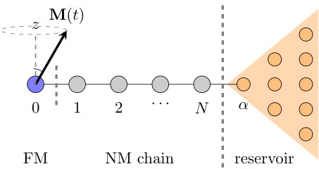 Figure 1
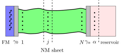 Figure 2
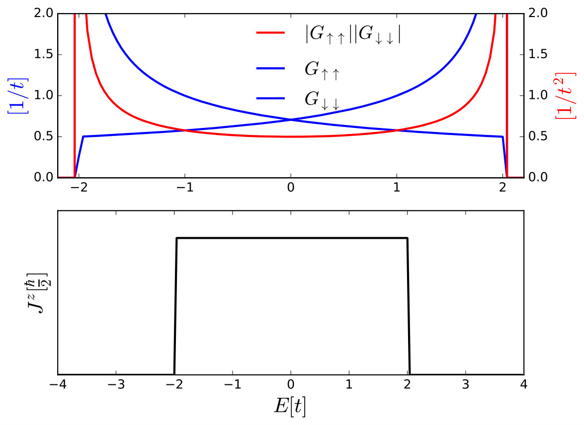 Figure 3
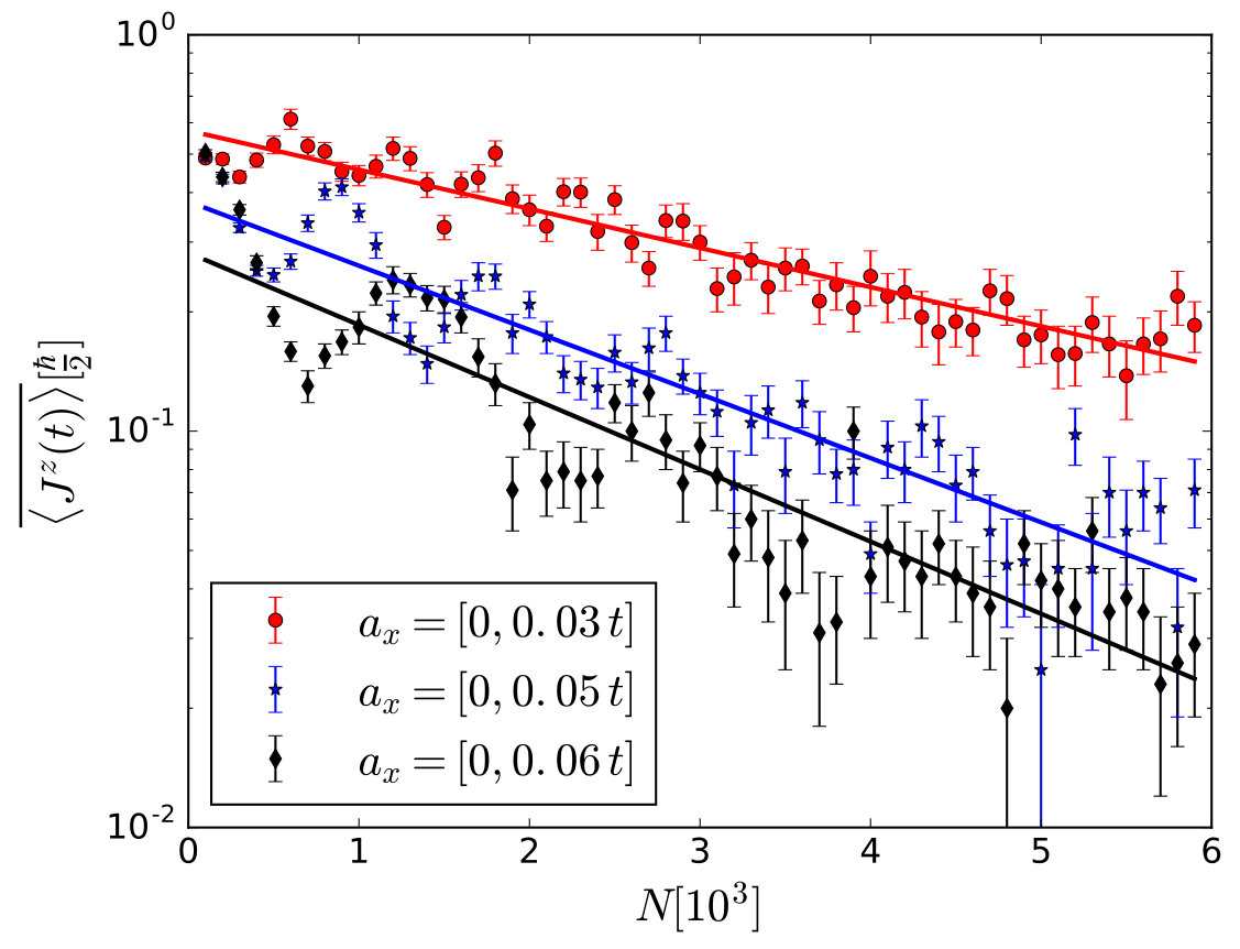 Figure 4
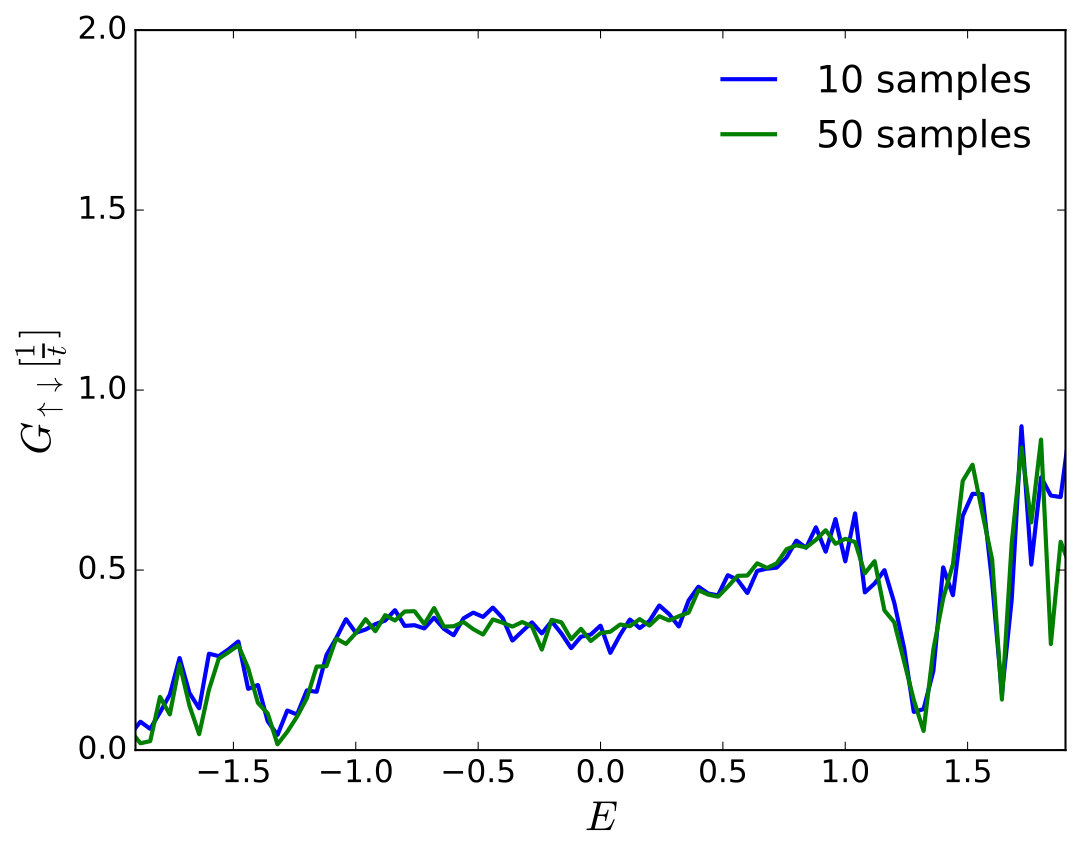 Figure 5
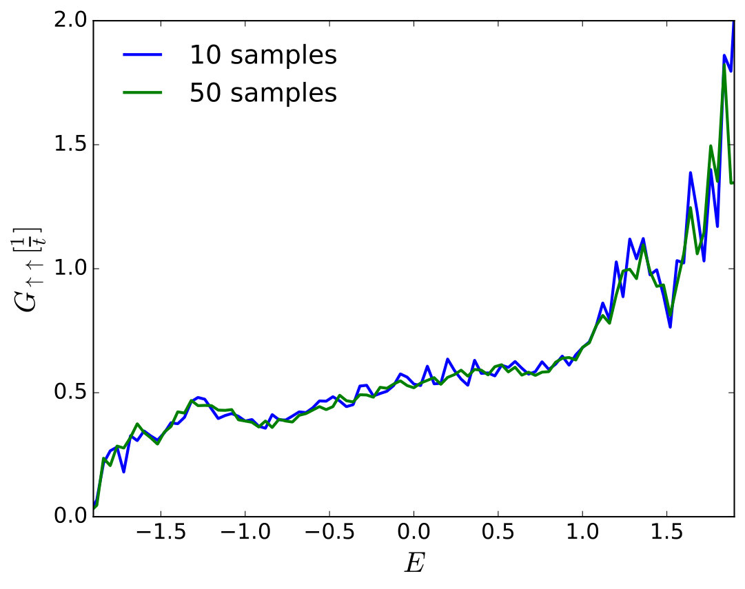 Figure 6
Peer Reviews
No public reviews on file for this paper yet. If you reviewed it on a platform where reviews are public (OpenReview, ICLR, NeurIPS, ICML), you can paste yours below so the community can read it here.
Videos
No videos yet. Explain this paper in a talk, walkthrough, or lecture? Add one.
Microscopic formulation of dynamical spin injection in
ferromagnetic-nonmagnetic heterostructures
Amin Ahmadi
Department of Physics, University of Central Florida, Orlando, FL 32816, USA
Eduardo R. Mucciolo
Department of Physics, University of Central Florida, Orlando, FL 32816, USA
Abstract
We develop a microscopic formulation of dynamical spin injection in heterostructure comprising nonmagnetic metals in contact with ferromagnets. The spin pumping current is expressed in terms of Green’s functions of the nonmagnetic metal attached to the ferromagnet where a precessing magnetization is induced. The formulation allows for the inclusion of spin-orbit coupling and disorder. The Green’s functions involved in the expression for the current are expressed in real-space lattice coordinates and can thus be efficiently computed using recursive methods.
I Introduction
One of the key elements in any implementation of spintronics is an efficient source of spin current.flatte-spintronic-Challenge Among the different methods available, dynamical spin injection from a ferromagnet metal (FM) into an adjacent nonmagnetic metal (NM) has been theoretically proposed Brataas_Spin_battery and experimentally observed.mizukami_exp_pump ; saitoh_pump ; Azvedo_SP_experimental ; Heinrich_SP_experimental ; mosendz_pump In this method, in addition to a longitudinal static magnetic field, an oscillating transverse magnetic field is applied, inducing a magnetization precession in the FM. Most of the angular momentum transferred to the FM by the oscillating field is dissipated through spin-relaxation processes in the bulk, but a small part survives as a spin current injected into the NM.
The exotic electronic properties of graphene have captured the attentions of the physics community since the first experiments with this material.geim ; deheer High mobility and a long spin-relaxation length are features that make graphene a promising passive element for spintronics.yang-Gr-relaxation In addition, the enhancement of spin-scattering processes in graphene by adatoms or defects,Hernando_spinRelaxationGr which yields spin Hall Kane_SHE_Gr and the inverse spin Hall effects, has led to proposals of graphene-based spin-pumping transistors.Ferreira_Gr_spinPump_transistor ; semenov-Gr-transistor
Recent experimental studies singh_spin_pumping_extended_Gr ; Singh_Spumping_fitInterface show an increase in the damping of the ferromagnetic resonance (FMR) when a graphene sheet is placed in contact with a FM subject to an oscillating magnetic field. One interpretation of phenomenon is that part of the precessing magnetization leaks into the graphene sheet as a spin current, effectively leading to another channel of magnetization damping in addition to the relaxation mechanisms existing in the bulk of the FM.
A time-dependent scattering theory brataas_1 ; Brataas_Spin_battery based on the general theory of adiabatic quantum pumping Buttiker_quantum_pump relate the increase in the FMR damping to the magnitude of a phenomenological mixing conductance parameter; further effort is necessary to describe microscopically the process of spin pumping into two-dimensional (2D) materials, as well as to properly quantify the spin current in terms of materials and interface parameters. A recent study Bauer_2Dpumping applied the time-dependent scattering theory to spin pumping in a insulating ferromagnet laid on top of a 2D metal. While insightful, this approach is not suitable for including disorder and spatial inhomogeneities such as adatoms; and when applied to graphene, it was confined to the vicinity of the neutrality point.
In this paper we develop a microscopical formulation of spin pumping from a FM into a NM material. Both the atomic structure of the materials and the particular geometry of the system can be taken into account exactly in this formulation. The spin current expression is written in terms of the Green’s function of the NM portion, allowing one to apply efficient recursive numerical methods for the computation of spin currents.eduardoRGF Another advantage of the formulation we present is the possibility to include accurate, microscopic models of spin-orbit coupling in the NM portion, as it relies on a spatial tight-binding representation of the system.
Another aspect that can be addressed with this formulation is the distinction between the angular momentum that relaxes at the interface and the part that flows into the NM. As it was shown in the experiment by Singh and coauthors,Singh_Spumping_fitInterface where a FM was laid on top of a graphene sheet, even without graphene protruding away from the FM (when no spin current injection is possible), the enhancement of damping is significant. This enhancement has been associated with two-magnnon scattering at the interface.hurben_2_magnnon However, in systems where graphene protrudes away from the FM, an extra damping has been measured due to the flow spin current into graphene. An atomistic study of such phenomenon is needed to discriminate the contribution of spin current from the surface relaxation in the enhanced damping.
This paper is organized as follows. In Sec. II, we use a one-dimensional tight-binding chain coupled to a magnetic site to introduce the time-dependent boundary condition problem and to derive an expression for the spin current based on an equation-of-motion formulation. The definition of charge and spin currents appropriate to the problem in hand are discussed in Sec. III. We apply the formulation to a zero-length system in Sec. IV and a finite-length chain in Sec. V. In Sec. VI the general expression for the spin current in the 2D system, including spin-orbit mechanisms is derived. In Sec. VII we summarize the results and point to future work. Details of the formulation and some derivations are presented in the Appendices.
II One-dimensional model
In this paper we address the problem of spin pumping in low-dimensional materials in contact with a FM where a precessing magnetization is induced. In such systems, itinerant electrons travel from the NM portion into the FM with a random spin orientation and back. The magnetization of FM changes the orientation of the spin of the returning electrons, and angular momentum leaks out of the FM and into the NM region as a spin current. To model such a hybrid FM/NM system, the FM region can be viewed as a time-dependent boundary condition to the NM region.
We begin by considering the idealized situation of a one-dimensional system, see Fig. 1. We adopt the transport formulation developed by Dhar and Shastry shastry as the starting point and extend it to include spin-dependent and time-dependent boundary conditions in the special case of a single reservoir attached to the nonmagnetic metal region.
Consider a one-dimensional chain where the site at is connected to a magnetic site at as shown in Fig. 1. At the magnetic site, itinerant electrons interact with the time-dependent magnetization of the FM,
[TABLE]
The dynamics of the magnetization is determined by the Landau-Lifshitz-Gilbert equation, where a damping term is introduced phenomenologically to account for magnetization loses.spc-book Here, we assume that Eq. (1) describes the stationary state of the magnetization and includes any damping. The opposite end of the chain, at the site , is connected to a reservoir via a site . A hopping term describes the itinerant electronic motion along the chain, where no spin-orbit mechanism is present at this point. The Hamiltonian of each segment reads
[TABLE]
[TABLE]
and
[TABLE]
where . The fermionic operators , , and act on the magnetic, chain, and reservoir sites, respectively and obey the standard anticommutation relations. are Pauli matrices. The parameters describe the hopping amplitude between neighboring sites and in the chain and could be spin dependent; in the absence of spin-orbit coupling, . The on-site potential is included to account for inhomogeneities in the chain. Finally, the matrix elements describe the site connectivity in the reservoir, which can be complex.
The coupling between the magnetic site and the chain and between the chain and the reservoir are assumed spin independent and are given by the Hamiltonians
[TABLE]
and
[TABLE]
respectively.
II.1 Equations of Motion
Equations of motion for the fermionic particle operators are obtained using the standard Heisenberg equation of motion, e.g., , where
[TABLE]
(we assume ). To simplify the notation, the time-dependent and time-independent amplitudes in Eq. (2) resulting after the insertion of Eq. (1) can be cast as frequency parameters and . We then obtain
[TABLE]
for the magnetic site and
[TABLE]
[TABLE]
with , and
[TABLE]
for the chain sites. In the expressions above, we introduced the spinor particle operators , , and and the matrices and .
For the equations of motion of the reservoir operators, we get homogeneous equations for the bulk and an equation containing an inhomogeneous term due to the coupling to the chain,
[TABLE]
and
[TABLE]
Combining Eqs. (12) and (13), we can express the general solution for the operator of the site with spin state in the integral form
[TABLE]
where the homogeneous part of the solution,
[TABLE]
plays the role of a noise-like term and the inhomogeneous part in Eq. (14) is dissipative in nature.shastry In Eqs. (14) and (15), denotes the retarded Green’s function of the decoupled reservoir and reads
[TABLE]
where are the single-particle eigenfunctions of the reservoir with eigenenergy (see Appendix A).
In the following, we assume that at a time the reservoir is in thermal equilibrium, such that
[TABLE]
where , is the Fermi-Dirac distribution, and and and the reservoir’s temperature and chemical potential, respectively (we assume ).
II.2 Fourier Transform of the Equations of Motion
It is useful to express the equations of motion in frequency domain. For that purpose, let us use the following convention for the Fourier transform of the particle operators and other time-dependent terms:
[TABLE]
[TABLE]
[TABLE]
[TABLE]
and
[TABLE]
Inserting these definitions into Eqs. (8) to (15), we obtain
[TABLE]
[TABLE]
[TABLE]
with ,
[TABLE]
and
[TABLE]
where the Fourier transform of the time-dependent part of the Hamiltonian is given by the expression
[TABLE]
with , and . Notice that is a matrix in spin space.
III Charge and Spin Currents
The expression for the charge current follows from the continuity equation in a discrete one-dimensional lattice,
[TABLE]
where is the charge density operator at the site (both the electron charge and the lattice constant are assumed to be unity). Using the equation of motion for , the particle current operator between sites and can be cast as
[TABLE]
Let us first consider the case when no spin-orbit coupling is present in the chain, namely, when is diagonal. Equation (30) gives us the total charge current as a sum of spin up and down currents at the site . However, to obtain the local spin current we need to keep in mind that when an electron with spin up is moving to the left, it produces an effect equivalent to an electron with spin down moving to the right as far as the transfer of angular momentum is concerned. In both cases, up spin angular momentum is transferred to the right. A general expression for spin continuity can be introduced by using the rate of change of magnetization and the conservation of angular momentum,spc-book
[TABLE]
where the spin density at the site is defined as and is the spin current operator between sites and ,note
[TABLE]
which is Hermitian: .
Now let us consider the case when there is spin-orbit coupling in the chain. In general, an external torque acting on the spin density at each site has to be included. The source torque can be due to on-site spin scattering process or to spin-orbit terms that cannot be reduced to the divergence of a current. Equation (32) still holds for a system with spin-orbit interactions, but an extra source torque term due to on-site spin scattering processes is needed in the continuity equation (31), which must be replaced by
[TABLE]
where the torque at site is defined as
[TABLE]
In Ref. SpinCurrent-definition, it was pointed out that the proper definition of spin current at the macroscopic level requires adding a contribution from the local external torque, such that Eq. (31) is restored. In other words, the external torque must be absorbed into the current expression. However, the microscopic nature of our model enables us to distinguish between the transfer of angular momentum either as spin currents or as a conversion to the other degrees of freedom. Therefore, we will adopt Eq. (32) even when spin-orbit coupling is present. In fact, the proper definition of the spin current in the presence of spin-dependent processes has been a source of debate in the literature rashba-sd ; tokatly-sd ; sonin1-sd ; sonin2-sd . One aspect that makes the definition nontrivial is the existence of intrinsic nondissipative background currents. In such systems, even without any dynamical source of current or spin chemical potential difference, a spin current can flow. As Sonin sonin1-sd ; sonin2-sd pointed out, regardless of the definition of the spin current, a source torque term is needed to compensate for the tranfer of spin angular to orbital angular momentum. In this paper we adopt Eq. (32) as the spin current expression. We return to discuss this definition in Sec. V.1 when we deriving an expression for the current in the presence of spin-orbit interaction.
The Fourier transform of the spin current between sites and of the chain takes the form
[TABLE]
Notice that, in Fourier space, the current is no longer Hermitian; instead, it satisfies . In particular, the components of the current can be written as
[TABLE]
where
[TABLE]
and .
Because of the harmonic nature of the precessing magnetization at the site, the expectation value of the Fourier transform of the spin current can be cast as a sum over multiples of the oscillation frequency , namely,
[TABLE]
where and is an integer. The stationary (dc) spin current can then be directly related to the zeroth harmonic component,
[TABLE]
IV Spin Pumping in the Absence of a Chain
For the sake of simplicity, we first evaluate the spin current for the case , when the reservoir is directly connected to the magnetic site. The study of the zero-length chain gives us some insight into the behavior of spin pumping currents and serves to guide us in derivations involving finite-length chains. Following Eq. (37), the spin- component of current in Fourier space reads (the site index can be dropped)
[TABLE]
where . The equations of motion for the chainless case can be obtained from Eqs. (II.2) and (27),
[TABLE]
and
[TABLE]
We can use Eq. (44) to eliminate from the expression of the spin- component of the current, , by replacing with and with in Eq. (37),
[TABLE]
recalling that . We can also substitute Eq. (44) into the the right-hand side of Eq. (43) to get
[TABLE]
where the static and the dynamic parts of the Hamiltonian are
[TABLE]
and
[TABLE]
respectively. The self energy due to the reservoir is given by
[TABLE]
and denotes the identity operator in spin space. Further simplification is possible by treating the right-hand side of Eq. (46) as a nonhomogeneous term and by writing the magnetic-site particle operator in terms of the fully-dressed Green’s function of that site,
[TABLE]
where
[TABLE]
Thus, we can express the magnetic-site operator entirely in terms of the noise-like operator . In the limit of , it is possible to show that the correlation function for is diagonal in spin and frequency (see Appendix B),
[TABLE]
where and is the reservoir’s density of states at the site ,
[TABLE]
Using Eqs. (52) and (50), one arrives at the following expression for the expectation value of the spin- component of the current:
[TABLE]
where and are functions of the magnetic-site Green’s functions , with ,
[TABLE]
and
[TABLE]
As we argue in Sec. IV.1, from the perturbative expansion of the Green’s function in powers , we know that even terms are diagonal in both spin and frequency, while odd terms are only nonzero when they involve opposite spin indices. Therefore, in general, one can write
[TABLE]
leading to
[TABLE]
It is then useful to rewrite in terms of same-spin-state and opposite-spin-state Green’s functions, namely,
[TABLE]
Using the Green’s function relation
[TABLE]
it is possible to show that the first term in the integrand on the right-hand side of Eq. (60) cancels exactly, leading to
[TABLE]
which is the central result of this Section.
Following similar steps, one can derive expressions for the other spin components of the current. The results can be combined into a single expression that generalizes Eq. (55), namely,
[TABLE]
where
[TABLE]
and
[TABLE]
IV.1 Perturbative Expansion in
In most situations of experimental relevance,ando-spinInjection ; ando-sI2 the transverse amplitude of time-dependent field driving the magnetization precession in the FM is much smaller than the longitudinal static component, resulting in . We consider this regime and expand the magnetic-site Green’s function in powers of , namely, in powers of the time-dependent Hamiltonian term :
[TABLE]
The zeroth-order (static) magnetic-site Green’s function is obtained by solving Eq. (51) when is absent, yielding
[TABLE]
where
[TABLE]
and . Thus, the zeroth-order Green’s function is diagonal in spin space.
The first-order Green’s function has only off-diagonal spin terms,
[TABLE]
while the second-order Green’s function recovers the spin-diagonal structure of the zeroth-order case,
[TABLE]
The spin dependence of higher order contributions to the Green’s function repeats this pattern: diagonal for even orders and off-diagonal for odd orders. In addition, even orders are also diagonal in the frequency variables.
IV.2 Spin Current Components
From the final expression for the spin- state component of the current, Eq. (62), and the expansion of the Green’s function up to second order in , one finds the following expression for the -component of the spin current:
[TABLE]
Since only the zero-frequency component is nonzero, upon returning to the time representation and utilizing Eq. (41), this relation yields a nonzero dc current, namely,
[TABLE]
where we have symmetrized the frequency integrand for convenience.
We notice that inverting the static magnetic field and the direction of precession (e.g., and ) flips the spin of the zeroth-order Green’s function . As a result, the spin current reverses its direction. This is expected on the basis of time-reversal symmetry. Moreover, at zero precession or zero transverse magnetic field, the spin current vanishes.
Considering now the component of the integral in Eq. (64), we obtain
[TABLE]
Notice that all terms contain opposite-spin-state Green’s functions, thus vanish in even powers in but are -dependent in odd powers of . As a result, in the time domain, oscillates and, upon averaging over one precession period, it vanishes. A similar argument can be used to show that vanishes as well. Therefore, all transverse components of the spin current vanish when averaged over time.
IV.3 Interface Parameters
The dynamics of the FM magnetization in the adiabatic approximation is governed by the Landau-Lifshitz-Gilbert (LLG) equation,
[TABLE]
where is the magnetization unit vector, is the gyromagnetic ratio, is the effective magnetic field (including the external magnetic field and the local demagnetization field), and is the Gilbert damping parameter. In the absence of any contact between the FM and a NM, the relaxation of the magnetization occurs entirely through processes internal to the FM, which are phenomenologically accounted for by the parameter . When a NM is brought in contact with the FM, the magnetization relaxation can also happen through angular momentum leaking into the NM as a spin current. To account for this contribution, consider that the effective magnetic field applied to the FM to be of the form
[TABLE]
where is the static component of the field while and are the time-dependent components. Following the scattering theory of spin pumping,Brataas_Spin_battery the spin current can be expressed as
[TABLE]
where the mixing conductance is defined in terms of reflection matrices as
[TABLE]
with the sum taken over transverse conducting channels. Notice the similarity of the right-hand side of Eq. (83) with the the Gilbert damping term in Eq. (81). One can absorb the angular momentum leakage contribution on the magnetization relaxation due to the spin current by substituting with in Eq. (81), where
[TABLE]
Here, is the Landé factor, is the total (bulk) magnetization of the FM, and (in most practical situations, the imaginary component of the mixing conductance can be neglected).
In the small precessing field approximation, , one can solve the LLG equation for the stationary solution of the dynamics of magnetization to get
[TABLE]
where
[TABLE]
and
[TABLE]
After substituting in Eq. (83), we arrive at
[TABLE]
We can combine this expression with that obtained in Sec. IV.2 for the spin current in terms of the system’s Green’s function, Eq. (79) to obtain an expression for the mixing conductance in terms of Green’s functions,
[TABLE]
In experiments, there are two standard approaches to quantify the spin pummping current and both are indirect. The first and most common consists of measuring the broadening of the FMR spectrum and utilizing Eqs. (85) and (89).mosendz_pump ; ando-sI2 ; heinrich-fmr1 The second is to infer the current magnitude through the observation of the inverse spin Hall effect (ISHE) in the NM when a sufficiently strong spin-orbit coupling is present.saitoh_pump ; mosendz-ishe ; ando-ishe Although, the latter seems more direct, the relation between the measured ISHE voltage and the actual spin current depends on various materials parameters which are often not accurately known.ishe-measurement Equation (90) provides a useful relation between the physical properties of medium where the spin current that is generated propagates to the enhanced broadening of FMR due to the angular momentum leakage. When generalized to higher dimensions, Eq. (90) provides a recipe for ab initio calculations of the Gilbert parameter.
V Spin Pumping with a Finite Chain
The formulation developed for the chain in Sec. IV can be extended to a finite-length chain. The equivalent to the equation of motion (46) for the particle operators in the chain can be written as
[TABLE]
where and we introduced . The matrix can be split into two contributions,
[TABLE]
where
[TABLE]
and
[TABLE]
Let us define the retarded Green’s function of the finite chain as . We can then solve Eq. (91) for the particle operator and write
[TABLE]
where . The Green’s function can be expanded in powers of similarly to Eq. (66). Since is diagonal in frequency, one can write the zeroth order term as
[TABLE]
Using this expression, the first-order contribution is found to be
[TABLE]
Similarly, for the second-order contribution we have
[TABLE]
Notice that in the absence of spin-orbit coupling in the chain, and the inelastic (off diagonal in frequency) contribution to the second-order Green’s function vanishes.
V.1 Current in the presence of spin-orbit coupling
If electrons experience no spin scattering in the chain, the spin -state current flows homogeneously from the magnetic site, along the chain, and into the reservoir without spin-orbit coupling. Thus, it can be shown that the spin current will remain the same as Eq. (79).
When spin-orbit is present, the spin current will vary along the chain. In this case, one is required to use Eq. (35) to compute the three components of the spin current at a given site . Let us focus on the component. Substituting Eq. (95) and its Hermitian conjugate into Eq. (35), we obtain
[TABLE]
where and denotes the retarded (advanced) Green’s function connecting sites and . Using the correlation function introduced in Eq. (52), we can take the expectation value of Eq. (LABEL:eq:J_z_spin) to obtain
[TABLE]
where the trace is over spin variables. Equation (LABEL:eq:J_z_spin_expec) is one of the main results of this paper. It provides a framework for computing the component of the spin current at any site within the chain that connects the magnetic site and the reservoir. Unfortunately, any further simplification of this expression is daunting. Similarly to the case where the reservoir is connected directly to the magnetic site, Sec. IV.1, we can use the perturbative expansion of the Green’s function in powers of . The result is still rather involved if the spin-dependent hopping amplitude is kept general and is not presented here.
A more compact expression can be obtained for the spin current between the last site of the chain and the reservoir, even in the presence of a general spin-orbit hopping amplitude. For that purpose, we take a step back, set in Eq. (35), and consider the component of the spin current operator,
[TABLE]
Using Eqs. (27) and (95), taking the expectation value, and using Eq. (52), we can rewrite Eq. (101) as
[TABLE]
The absence of a spin-dependent hopping amplitude in Eq. (102) makes it more amenable to an analytical treatment. Focusing on the dc component of the spin current, as shown in Eqs. (38) and (41), we expand the Green’s function harmonics of the precessing frequency , namely,
[TABLE]
Inserting this expansion into Eq. (102) and keeping only the terms corresponding to the dc limit, we obtain
[TABLE]
We can now use the relations
[TABLE]
where
[TABLE]
to find
[TABLE]
Combing Eqs. (104) and (107), recalling that and using Eq. (53), we arrive at
[TABLE]
Symmetrizing the frequency integration, we finally obtain the following expression for the dc spin current at the interface with the reservoir:
[TABLE]
where the trace is over spin indices. Notice that in the limit of zero pumping frequency (), the spin current goes to zero.
At this point, we can go back to the perturbative expansion of the Green’s functions in powers of and notice the following:
[TABLE]
and
[TABLE]
Since , by keeping only the leading term in powers of we obtain
[TABLE]
It is straightforward to verify that setting in Eq. (112) leads to Eq. (79). Notice that for , the current is proportional to ,
[TABLE]
Equations (109) and (113) are the main results of this section. Equation (109) can be employed to study dynamical spin pumping beyond the linear response approximation. Combining Eq. (113) with Eq. (83) enables an atomistic calculation of the macroscopic Gilbert parameter, which can be measured in FMR experiments.
To illustrate the results obtained so far, we performed numerical calculations of the chain Green’s function for chains of various lengths in the presence and absence of spin-dependent on-site potentials. In Fig. 2, the spin-diagonal components of the Green’s function across the chain, , and the total spin pumping current, , are plotted as functions of energy. A constant spin current over energy confirms that, in the absence of spin-scattering centers, the chain is a spin-degenerate ballistic propagating channel so long as the energy is within the energy band. In this case, the spin current is independent of the length of the chain.
Figures 4 and 3 show the energy dependence of the spin components of the chain’s average Green’s function when spin-polarized impurities are introduced but no spin-dependent hopping is present. In these simulation, and , where the amplitudes and are randomly and uniformly chosen in the intervals and , respectively. Here denotes the hopping amplitude in the lattice.
One of the key advantages of our formalism is that it can be utilized to compute the relaxation of the spin current over distance from the FM/NM interface due to spin-scattering processes in the NM region. For large enough systems, the diffusion length can be calculated.
The dependence of the average dc spin pumping current on the length of the chain is shown in Fig. 5 for the same random spin-dependent potential. Even after averaging over 300 samples, oscillations over the length due to interference remains. However, a clear exponential decay emerges, with a decay length of , , and lattice units for the three increasing disorder ranges of shown in the plot.
VI Extension to Two-Dimensional Systems
The spin pumping formulation developed in Secs. II, IV.2, and V can be extended to 2D systems. To do so, we imagine the magnetic region as a column of magnetic sites whose magnetizations precess in a synchronized way, corresponding to a single magnetic domain. The two-dimensional nonmagnetic region is sliced into columns and connected to a reservoir, see Fig. 6. We keep the same notation used for the one-dimensional finite-chain case and write the Hamiltonians of the different regions as
[TABLE]
for the magnetic region,
[TABLE]
for the nonmagnetic region, and
[TABLE]
for the reservoir. The Hamiltonians describing the coupling between magnetic and nonmagnetic regions (hereafter referred to as sheet), and between the nonmagnetic region and the reservoir are given by
[TABLE]
and
[TABLE]
respectively, where is the particle operator at the column containing the magnetic region (), is a matrix that describes the coupling between the magnetic region and the sheet, is the particle operator at the th sheet slice, which is connected to the neighboring -th slice by the matrix , is the number of sites in th slice, and is the coupling matrix between the th sheet slice and the reservoir. Finally, the particle operator acting on the sites in the reservoir that are connected directly to the sheet is given by .
The equations of motion read
[TABLE]
[TABLE]
and
[TABLE]
The Fourier transforms of the equations of motion result in expressions similar those obtained in Sec. II, namely,
[TABLE]
[TABLE]
and
[TABLE]
where is a vector with dimension of the surface sites in the reservoir and the Green’s function of the decoupled reservoir for slice reads
[TABLE]
In order to expand the Green’s function in powers of , we notice that, in spin space,
[TABLE]
which leads us to analogous relations to those derived in Sec. V for the finite chain.
In order to calculate the spin current along the sheet, we can use an expression identical to that introduced in Sec. III, namely,
[TABLE]
The only difference between this relation and Eq. (35) is that here there is an implicit sum over transverse sites. Using the orthogonality relation of one can derive an expression for the expectation value of the total spin current between the th and th slices as
[TABLE]
where the trace is over spin and transvese site variables,
[TABLE]
and denotes the retarded (advanced) Green’s function connecting the and slices. A detailed derivation of Eq. (132) is provided in Appendix D.
Similar to the 1D chain, we can go further to calculate the current at the chain-reservoir interface and expand the Green’s function harmonics of the precessing frequency ,
[TABLE]
to derive
[TABLE]
Equation (135) is the central result of this paper. This equation can be used to study dynamical spin pumping in FM/NM setups beyond the linear response. In the slow-precession limit, combined with Eq. (83), it gives us a recipe for the calculation of the mixing conductance and the Gilbert parameter by solely knowing the microscopic structure of the NM system.
The formalism developed in this section has several advantages over the scattering formulation: (i) The detailed geometry of the FM/NM systems and physical properties of the NM can be taken into account by computing the appropriate Green’s function. (ii) Since the final expression for the spin current is written in terms of the surface Green’s functions, the recursive Green’s function technique eduardoRGF can be utilized for an efficient computational approach to the problem. (iii) Furthermore, since a spatial representation of the system is used in this formalism, systems with higher dimension and arbitrary geometry can be readily simulated.
VII Summary and Discussion
In this paper, we developed an atomistic model of spin pumping in hybrid ferromagnetic heterostructures. The spin current expression is given in terms of the Green’s function of the nonmagnetic portion. Motivated by the fact that, in experimental settings, the time-dependent component of the driving magnetic field is small and slow, we use a perturbative expansion to obtain a relation between the mixing conductance and the physical properties of spin-carrying medium. Among the advantages of this formalism are: (i) it provides a framework for including the atomic structure and geometry of the heterostructure, as well as local disorder and spin-orbit coupling mechanism, (ii) it yields an expression for the spin current in terms of Green’s function, which can be computed using efficient recursive computational methods, (iii) it allows us to model spin relaxation and the ferromagnet-nonmagnetic metal interface, and (iv) when applied to graphene, it is not limited to high doping.
In a future work we plan to apply this new computational tool to study dynamical spin injection in realistic ferromagnet-graphene heterostructures, and to extend the calculations to include a determination of the spin-Hall voltage across the graphene channel when spin-orbit coupling is included.
Acknowledgements.
We are grateful to C. Lewenkopf and A. Ferreira for insightful discussions. E.R.M. acknowledges the hospitality of the Instituto de F\a’isica at UFF, Brazil, where this work was initiated. This work was supported in part by the NSF Grant ECCS 1402990.
Appendix A Reservoir Green’s function
The retarded Green’s function of the decoupled reservoir is defined as
[TABLE]
Expanding the field operators in terms of single-particle energy eigenfunctions
[TABLE]
the retarded Green’s function of the reservoir can be written as
[TABLE]
Appendix B Noise-like correlator
We can rewrite the correlation function of the noise-like term in frequency space in terms of the fermionic operators in time using Eq (15),
[TABLE]
After substituting the expansion of decoupled reservoir’s Green’s function in terms of the reservoir’s eigenfunction, Eq. (16), we get
[TABLE]
Using the reservoir’s eigenfunction basis,
[TABLE]
and the orthogonality of the reservoir’s eigenfunctions, we obtain
[TABLE]
Using Eq. (17) and taking the limit we arrive at Eq. (52).
For 2D systems, the correlation function can be obtained in the same way:
[TABLE]
Using the orthonormal set of eigenfunctions of the reservoir,
[TABLE]
we can write
[TABLE]
when we set . We finally arrive at
[TABLE]
where and is the density of states matrix at the slice,
[TABLE]
Appendix C -component of the spin current
Substituting Eq. (44) into Eq. (42), we obtain
[TABLE]
Employing Eq. (50), we can derive the following relations:
[TABLE]
[TABLE]
and
[TABLE]
Putting these relations together with Eq. (153) one arrives at Eq. (55).
Appendix D Spin current for 2D systems
The fermionic particle operator in terms of the system Green’s function reads
[TABLE]
where is the number of sites in the slice . After substituting it into the current expression
[TABLE]
the expectation value of the first term in Eq. (158) becomes
[TABLE]
By applying the correlator we find
[TABLE]
We can follow the same approach to calculate the current at the chain-reservoir interface:
[TABLE]
The current expression can be written as
[TABLE]
which can be simplified to
[TABLE]
After substituting the fermionic operator in terms of the system’s Green’s function, the expectation value of the spin current becomes
[TABLE]
Similar to the 1D case, we expand the Green’s function in terms of the frequency difference,
[TABLE]
and following the same approach used in the 1D case, we get
[TABLE]
which leads to
[TABLE]
leading to
[TABLE]
The reference list from the paper itself. Each links out to its DOI / PubMed record.
- 1(1) D. D. Awschalom and M. E. Flatté, Nat. Phys. 3 , 153 (2007).
- 2(2) A. Brataas, Y. Tserkovnyak, G. E. W. Bauer, and B. I. Halperin, Phys. Rev. B 66 , 060404 (2002).
- 3(3) S. Mizukami, Y. Ando, and T. Miyazaki, Jap. J. Appl. Phys. 40 , 580 (2001).
- 4(4) E. Saitoh, M. Ueda, H. Miyajima, and G. Tatara, Appl. Phys. Lett. 88 , 182509 (2006).
- 5(5) A. Azevedo, L. H. Vilela Leo, R. L. Rodriguez-Suarez, A. B. Oliveira, and S. M. Rezende, J. Appl. Phys. 97 , 10C 715 (2005).
- 6(6) B. Heinrich et al ., Phys. Rev. Lett. 107 , 066604 (2011).
- 7(7) O. Mosendz, J. Pearson, F. Fradin, G. Bauer, S. Bader, and A. Hoffmann, Phys. Rev. Lett. 104 , 046601 (2010).
- 8(8) K. S. Novoselov, A. K. Geim, S. V. Morozov, D. Jiang, Y. Zhang, S. V. Dubonos, I. V. Grigorieva, and A. A. Firsov, Science 306 , 666 (2004).