Latent Gaussian Mixture Models for Nationwide Kidney Transplant Center Evaluation
Lanfeng Pan, Yehua Li, Kevin He, Yanming Li, Yi Li

TL;DR
This paper introduces a novel latent Gaussian mixture model to evaluate kidney transplant centers nationwide, improving the assessment of center effects by capturing heterogeneity and addressing distributional assumptions.
Contribution
It proposes a penalized likelihood estimation method for latent Gaussian mixture models and develops tests to determine the number of mixture components, enhancing center effect analysis.
Findings
Distributional assumptions affect center effect predictions.
The mixture model effectively captures heterogeneity among centers.
Simulation and real data validate the proposed approach.
Abstract
Five year post-transplant survival rate is an important indicator on quality of care delivered by kidney transplant centers in the United States. To provide a fair assessment of each transplant center, an effect that represents the center-specific care quality, along with patient level risk factors, is often included in the risk adjustment model. In the past, the center effects have been modeled as either fixed effects or Gaussian random effects, with various pros and cons. Our numerical analyses reveal that the distributional assumptions do impact the prediction of center effects especially when the effect is extreme. To bridge the gap between these two approaches, we propose to model the transplant center effect as a latent random variable with a finite Gaussian mixture distribution. Such latent Gaussian mixture models provide a convenient framework to study the heterogeneity among…
Click any figure to enlarge with its caption.
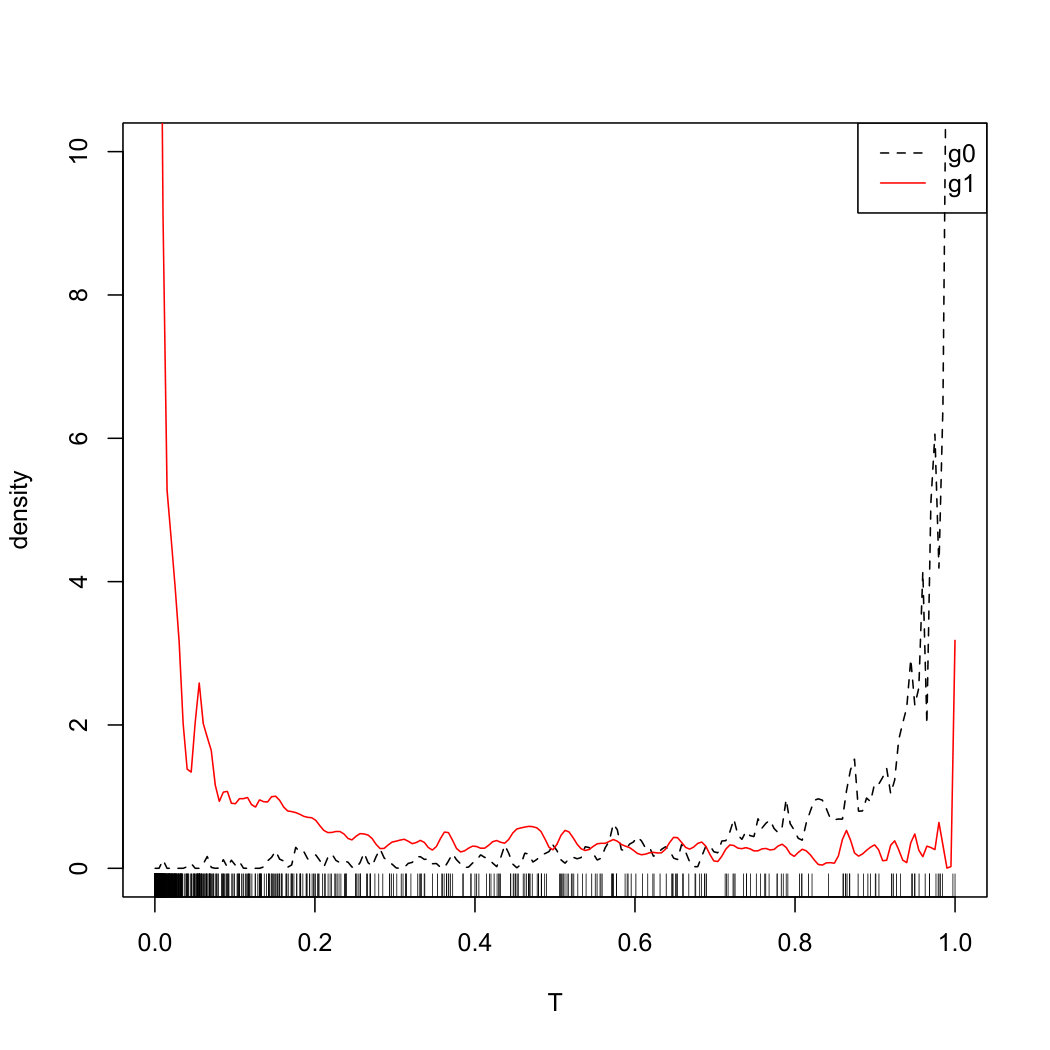 Figure 1
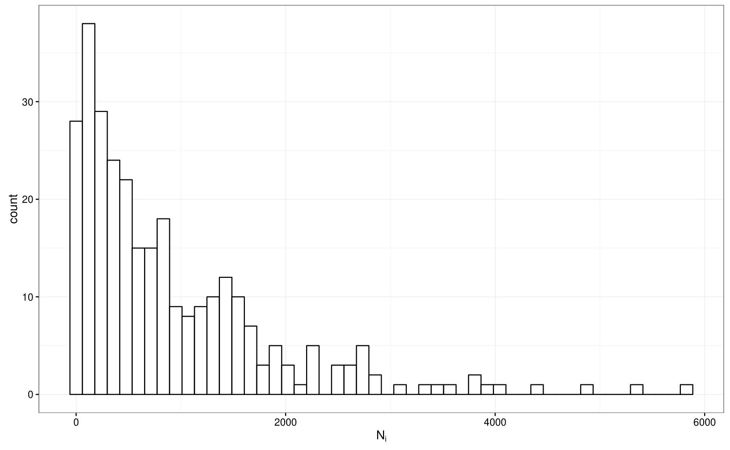 Figure 2
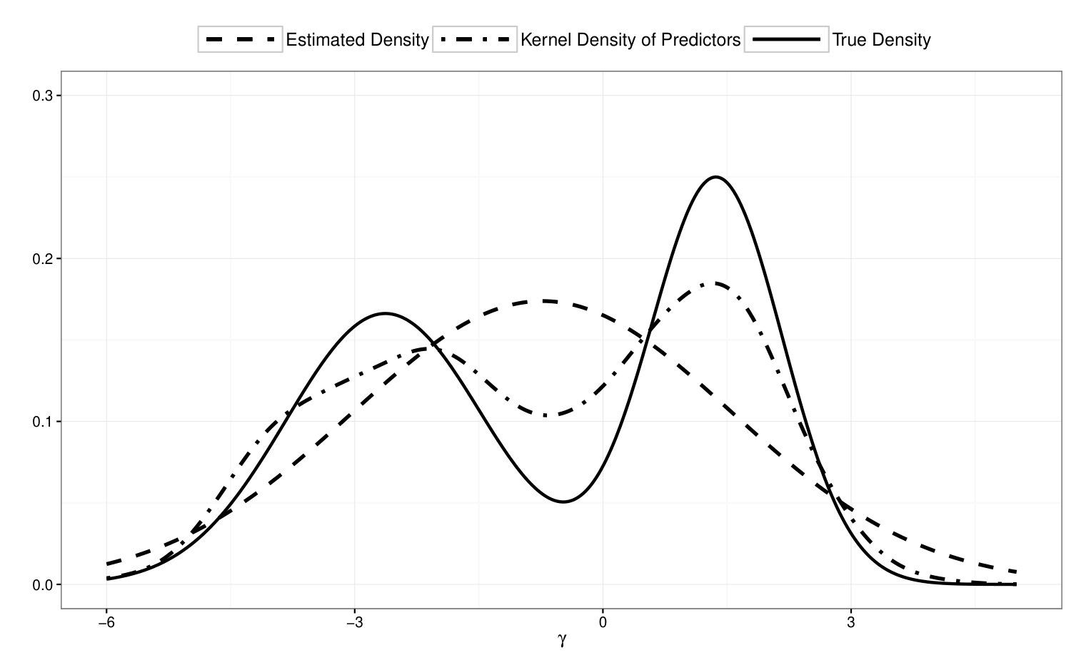 Figure 3
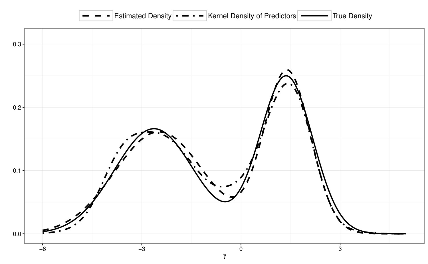 Figure 4
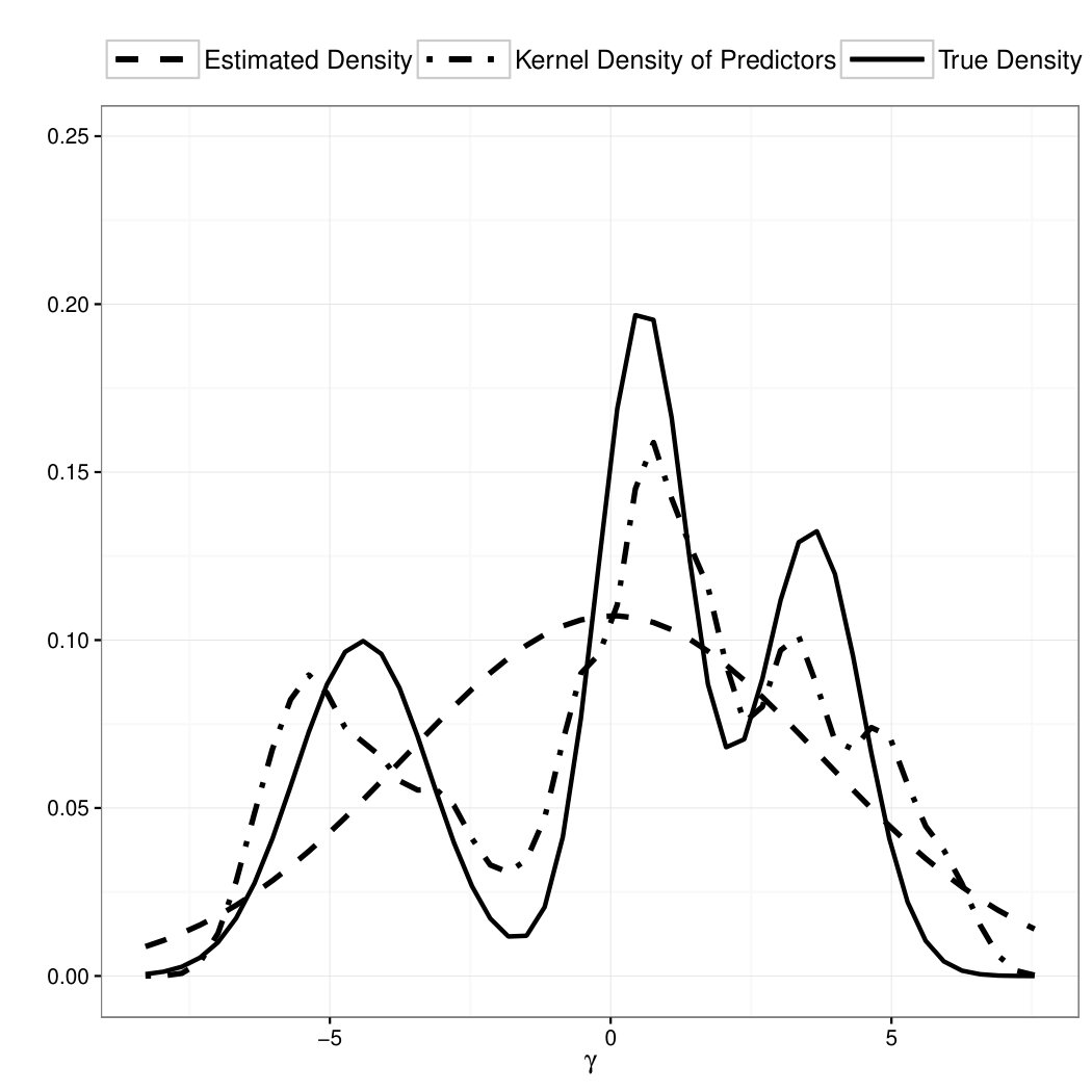 Figure 5
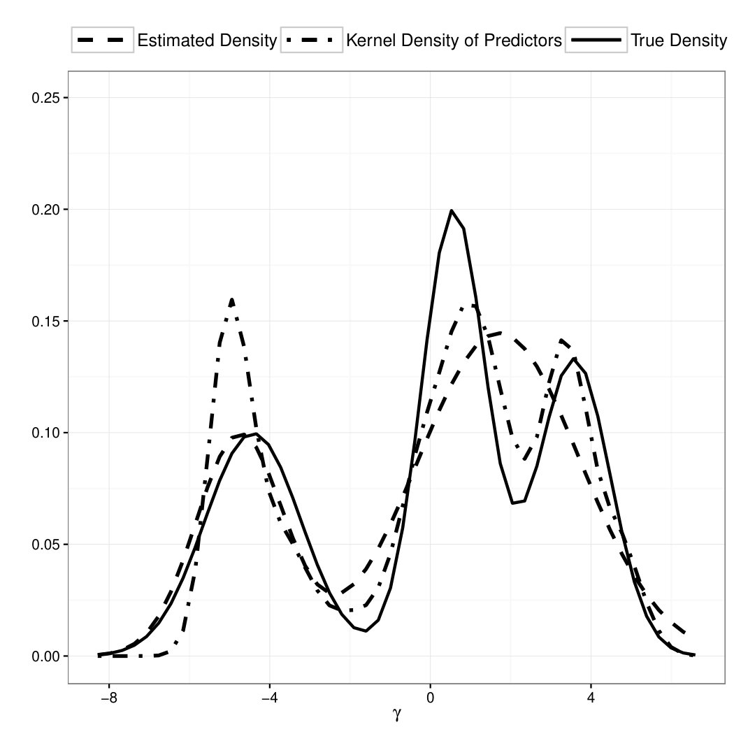 Figure 6
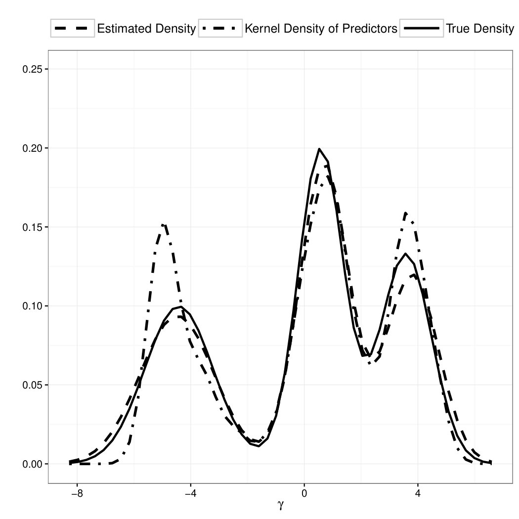 Figure 7
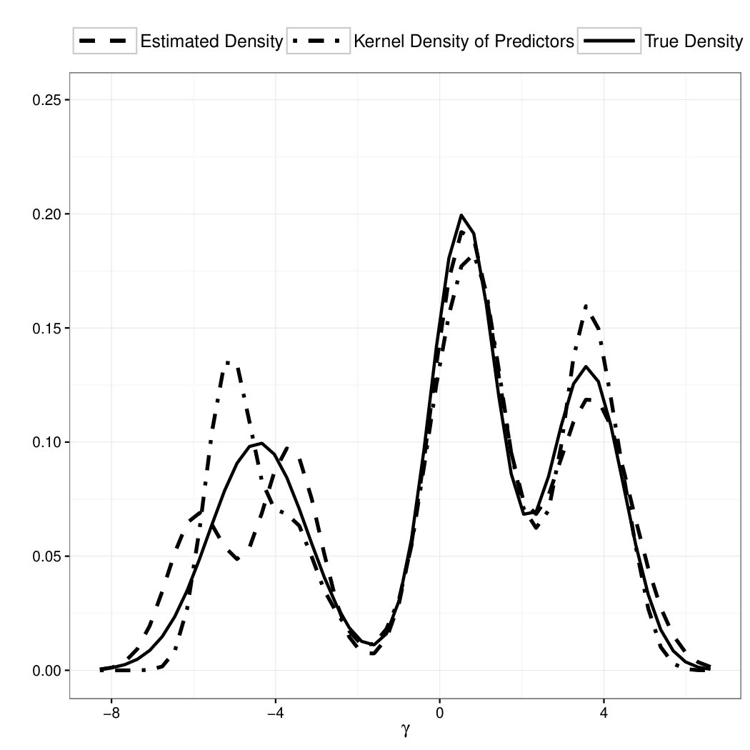 Figure 8
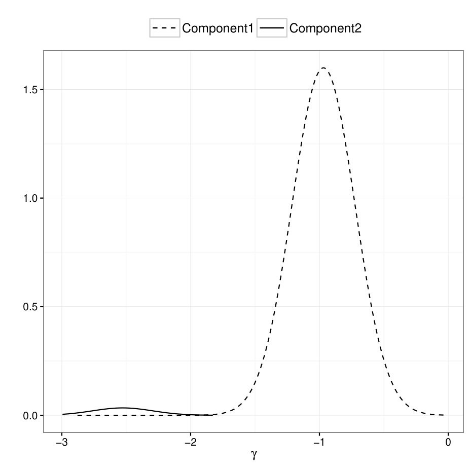 Figure 9
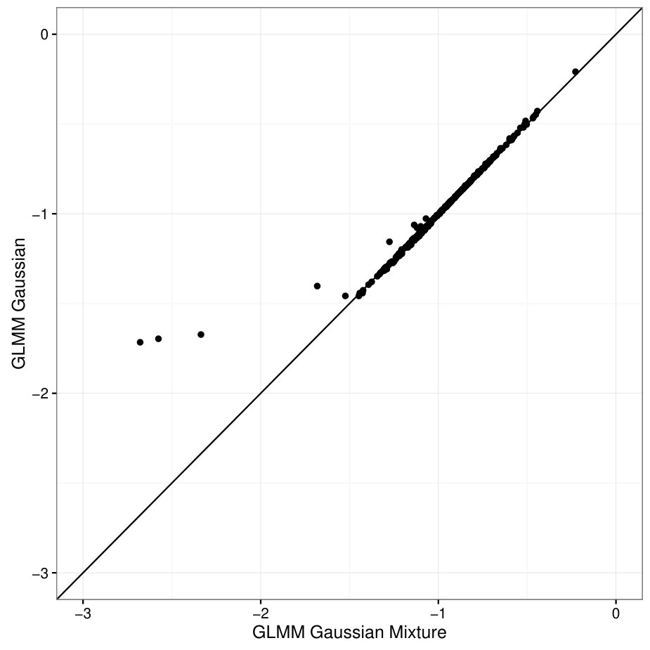 Figure 10
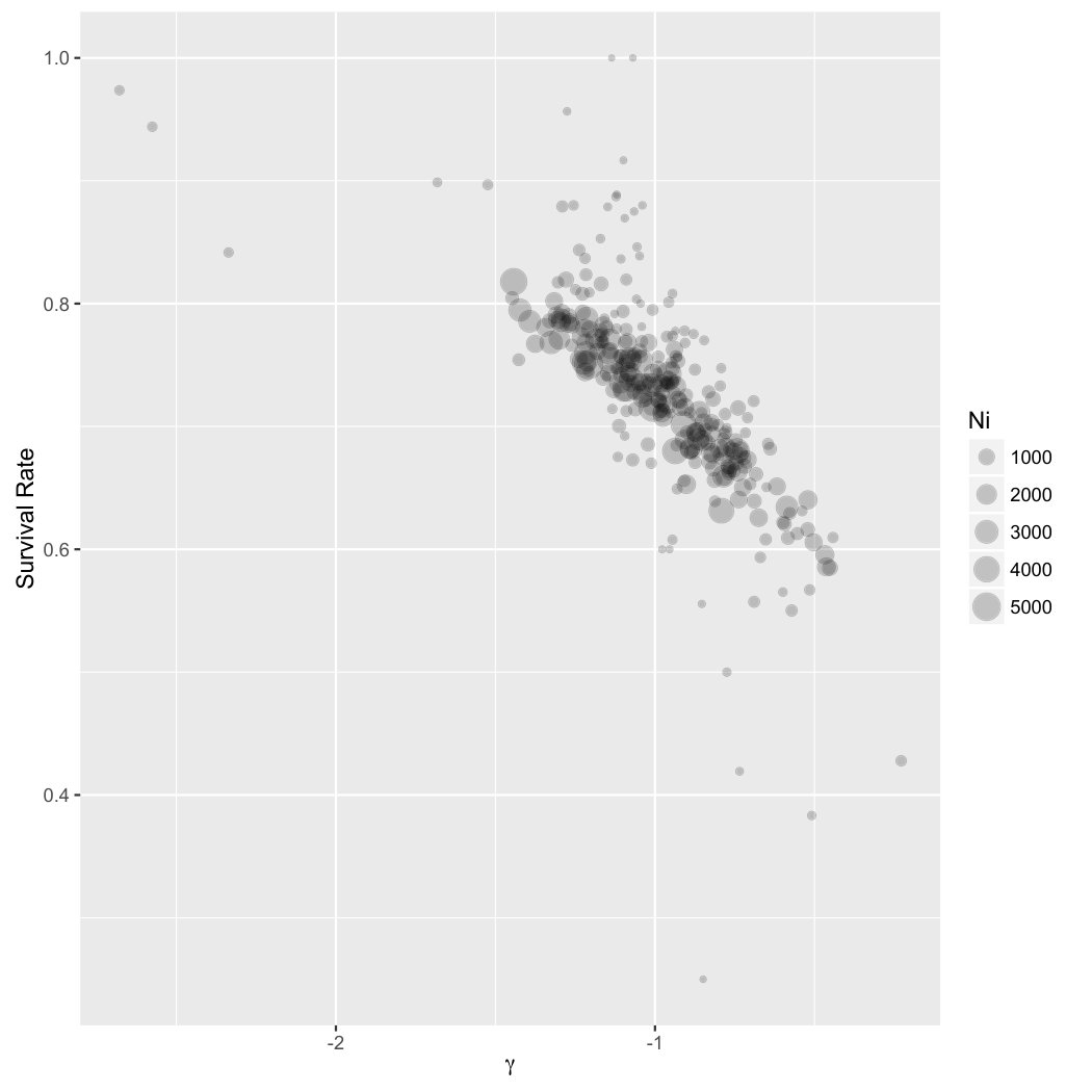 Figure 11
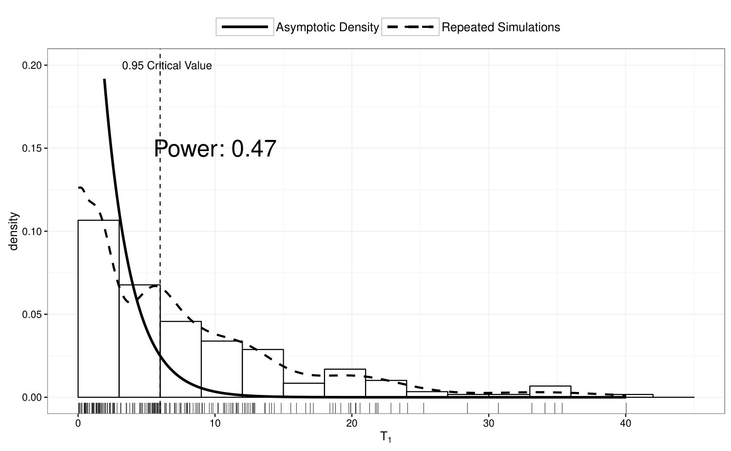 Figure 12
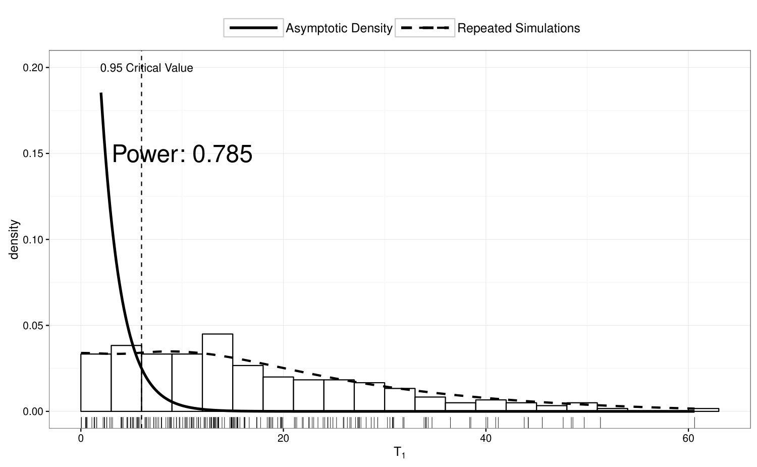 Figure 13
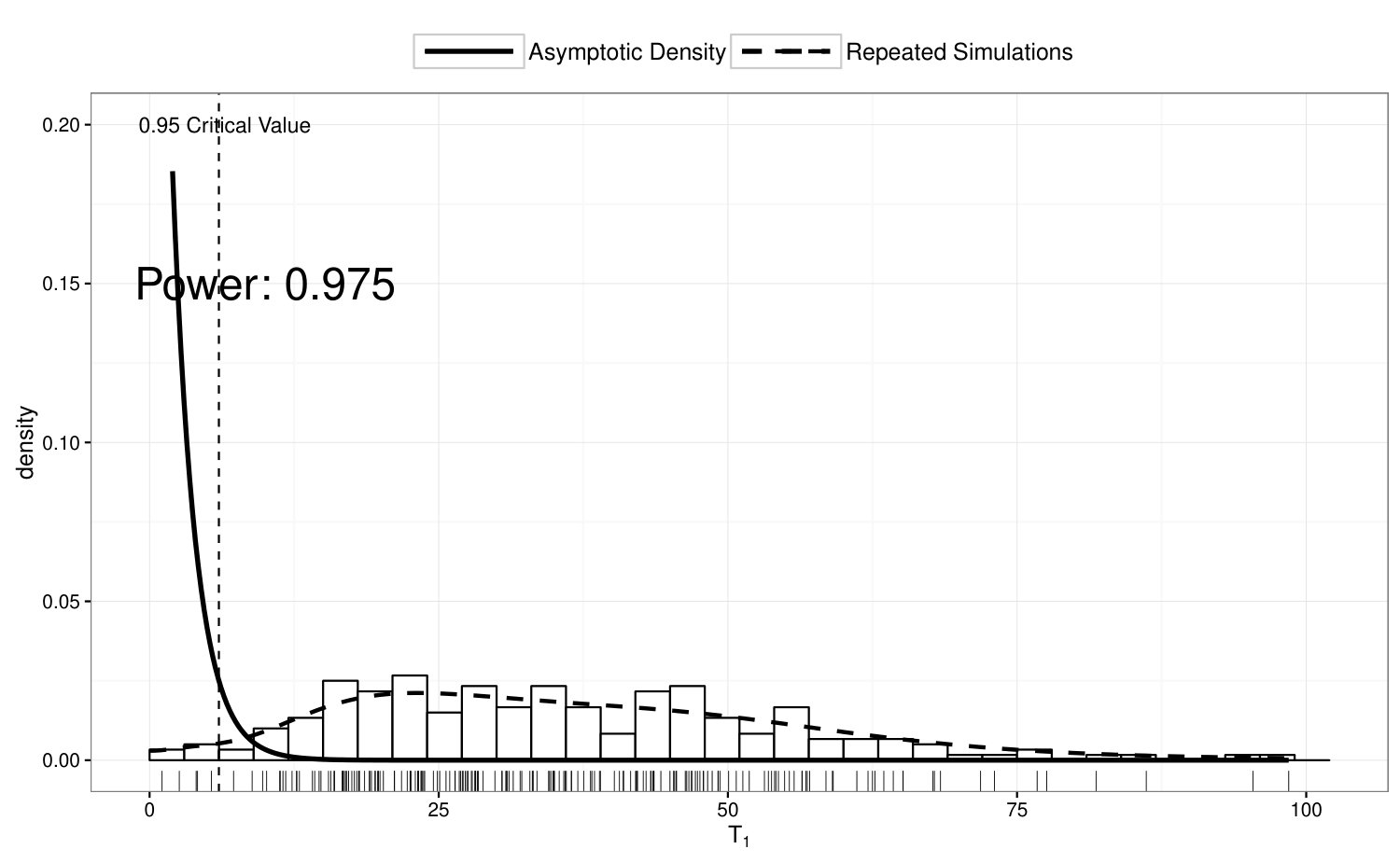 Figure 14
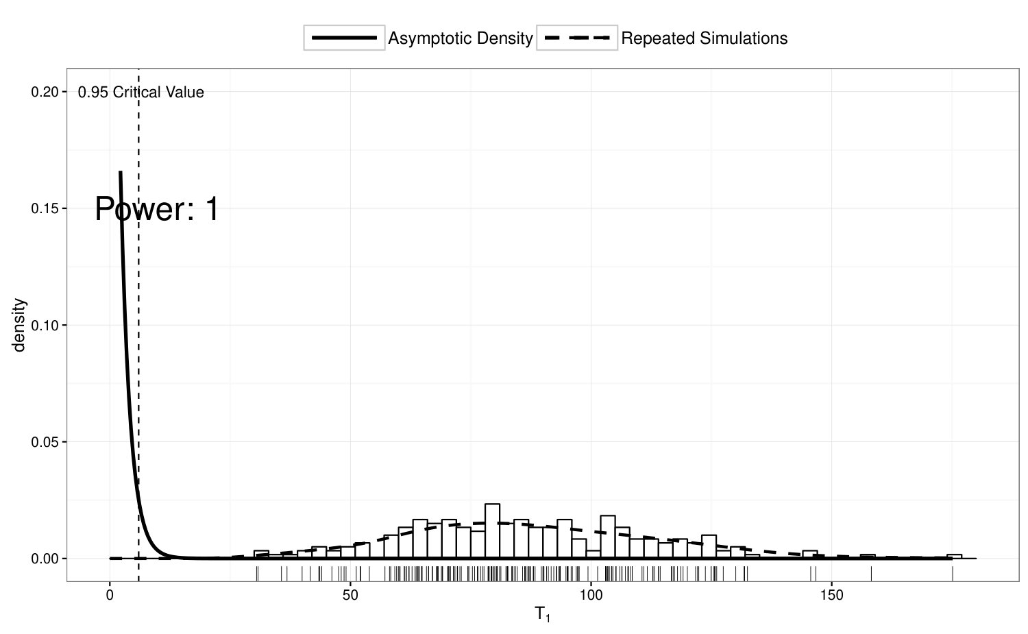 Figure 15
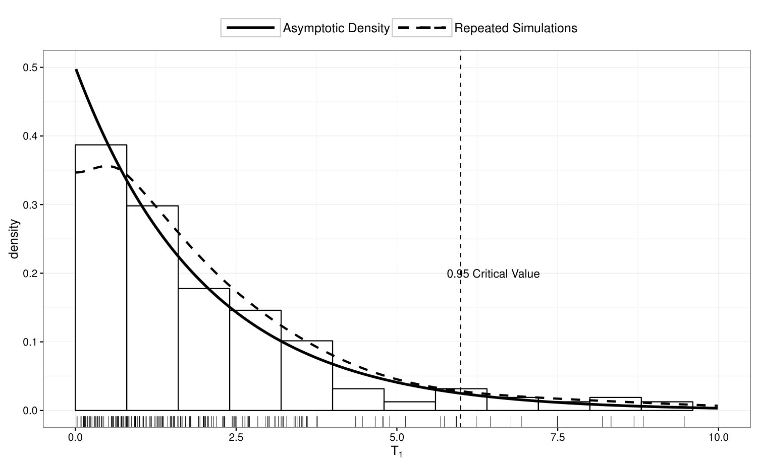 Figure 16
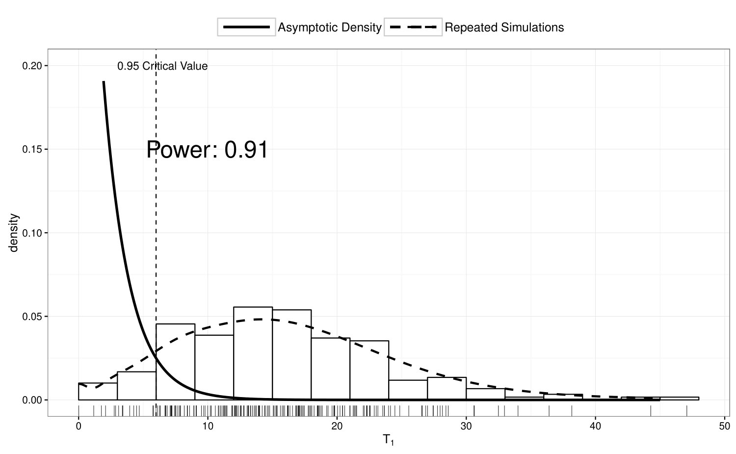 Figure 17
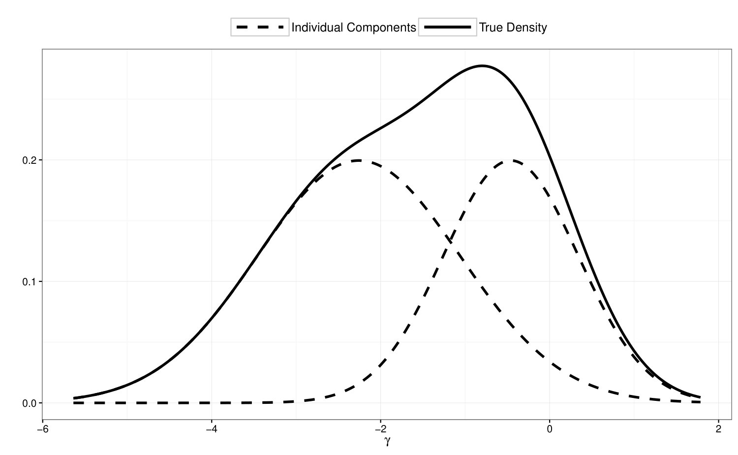 Figure 18
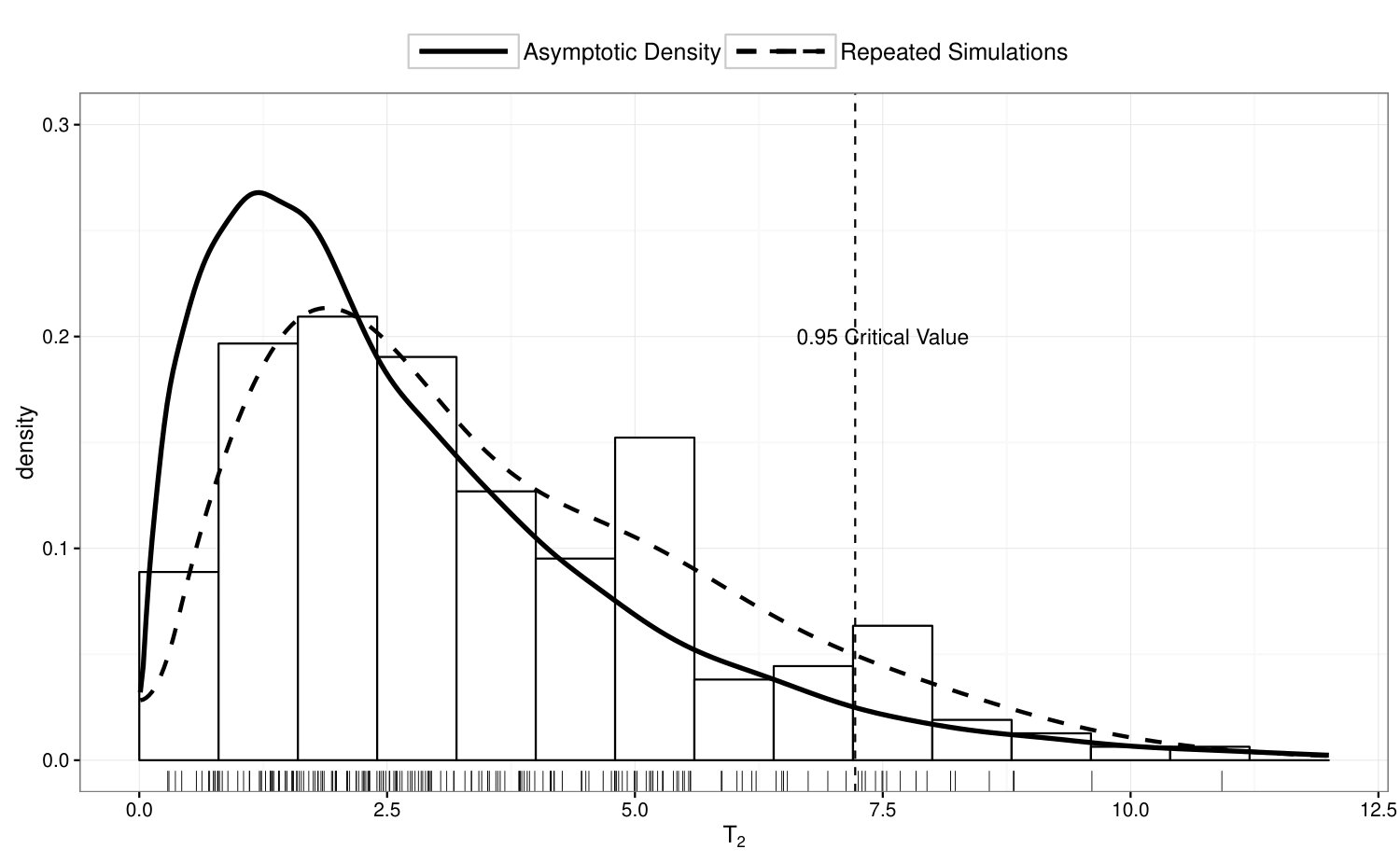 Figure 19
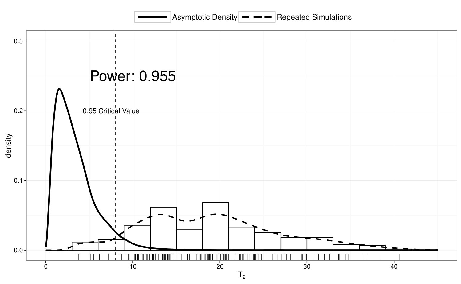 Figure 20
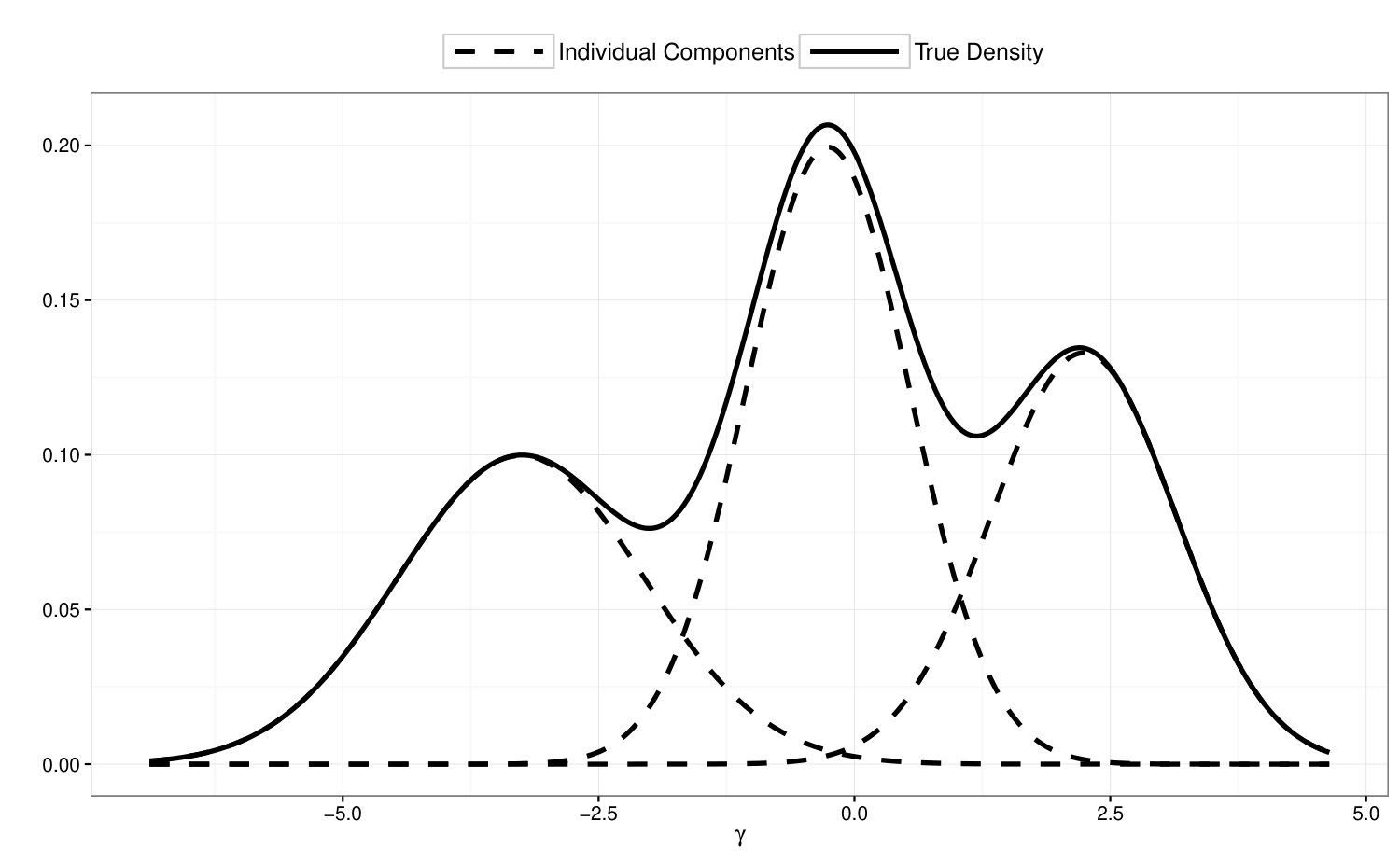 Figure 21
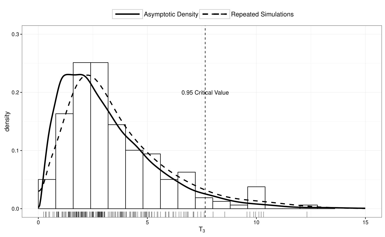 Figure 22
| Truth | Mean | Bias | Std | |
|---|---|---|---|---|
| 0.5000 | 0.4971 | -0.0029 | 0.0280 | |
| 0.5000 | 0.5029 | 0.0029 | 0.0280 | |
| -3.2598 | -3.2586 | 0.0012 | 0.1262 | |
| 0.7402 | 0.7401 | -0.0001 | 0.0752 | |
| 1.2000 | 1.1954 | -0.0046 | 0.1340 | |
| 0.8000 | 0.7960 | -0.0040 | 0.0630 | |
| 1.0000 | 1.0017 | 0.0017 | 0.0213 | |
| 1.0000 | 1.0006 | 0.0006 | 0.0225 |
| Truth | Mean | Bias | Std | |
|---|---|---|---|---|
| 0.3000 | 0.3016 | 0.0016 | 0.0244 | |
| 0.4000 | 0.3904 | -0.0096 | 0.0588 | |
| 0.3000 | 0.3080 | 0.0080 | 0.0596 | |
| -5.2598 | -5.2800 | -0.0202 | 0.2175 | |
| -0.2598 | -0.2652 | -0.0054 | 0.3472 | |
| 2.7402 | 2.6894 | -0.0508 | 0.3433 | |
| 1.2000 | 1.1821 | -0.0179 | 0.2664 | |
| 0.8000 | 0.8036 | 0.0036 | 0.1948 | |
| 0.9000 | 0.9286 | 0.0286 | 0.2516 | |
| 1.0000 | 1.0010 | 0.0010 | 0.0225 | |
| 1.0000 | 1.0038 | 0.0038 | 0.0226 |
| Simulation Model | Fitted Model | Mean | Std |
|---|---|---|---|
| Model 1 | GLMM Gaussian | 0.4167 | 0.0392 |
| GLMM Mixture | 0.3589 | 0.0361 | |
| Model 2 | GLMM Gaussian | 0.6988 | 0.0697 |
| GLMM Mixture | 0.5405 | 0.0581 |
| Estimate | Std. Error | -value | -value | |
|---|---|---|---|---|
| 0.019503 | 0.0003048 | 63.9869 | 1e-99 | |
| 0.007112 | 0.0002117 | 33.5890 | 1e-99 | |
| 0.030928 | 0.0094616 | 3.2688 | 0.0011 | |
| 0.077860 | 0.0154998 | 5.0232 | 1e-6 | |
| 0.120536 | 0.0129628 | 9.2986 | 1e-19 | |
| 0.225015 | 0.0148196 | 15.1836 | 1e-51 | |
| -0.270078 | 0.0146769 | -18.4016 | 1e-74 | |
| -0.526297 | 0.0127432 | -41.3003 | 1e-99 | |
| -0.632073 | 0.0138511 | -45.6334 | 1e-99 | |
| -0.800276 | 0.0130163 | -61.4824 | 1e-99 |
| Center id | lFDR | Sample Size | Survival Rate | |
|---|---|---|---|---|
| #287 | 0.0013 | -2.6784 | 114 | 0.973 |
| #10 | 0.0061 | -2.5753 | 125 | 0.944 |
| #28 | 0.0736 | -2.3364 | 120 | 0.841 |
Peer Reviews
No public reviews on file for this paper yet. If you reviewed it on a platform where reviews are public (OpenReview, ICLR, NeurIPS, ICML), you can paste yours below so the community can read it here.
Videos
No videos yet. Explain this paper in a talk, walkthrough, or lecture? Add one.
Taxonomy
TopicsBayesian Methods and Mixture Models · Liver Disease Diagnosis and Treatment · Statistical Methods and Bayesian Inference
Latent Gaussian Mixture Models for Nationwide Kidney Transplant Center Evaluation
Lanfeng Panlabel=e1][email protected] [
Yehua Lilabel=e2][email protected] [
Kevin Helabel=e3] [
Yanming Lilabel=e4] [
Yi Lilabel=e5] [ \thanksmarkd1 Department of Statistics & Statistical Laboratory, Iowa State University
\thanksmarkd2 School of Public Health & Kidney Epidemiology and Cost Center, University of Michigan, Ann Arbor
Abstract
Five year post-transplant survival rate is an important indicator on quality of care delivered by kidney transplant centers in the United States. To provide a fair assessment of each transplant center, an effect that represents the center-specific care quality, along with patient level risk factors, is often included in the risk adjustment model. In the past, the center effects have been modeled as either fixed effects or Gaussian random effects, with various pros and cons. Our numerical analyses reveal that the distributional assumptions do impact the prediction of center effects especially when the effect is extreme. To bridge the gap between these two approaches, we propose to model the transplant center effect as a latent random variable with a finite Gaussian mixture distribution. Such latent Gaussian mixture models provide a convenient framework to study the heterogeneity among the transplant centers. To overcome the weak identifiability issues, we propose to estimate the latent Gaussian mixture model using a penalized likelihood approach, and develop sequential locally restricted likelihood ratio tests to determine the number of components in the Gaussian mixture distribution. The fitted mixture model provides a convenient means of controlling the false discovery rate when screening for underperforming or outperforming transplant centers. The performance of the methods is verified by simulations and by the analysis of the motivating data example.
Clustering,
False discovery rate,
Health policy,
Locally restricted likelihood ratio test,
Penalized EM algorithm,
Latent variables,
keywords:
\setattribute
journalname \startlocaldefs
\endlocaldefs
, , ,
and
m3Correspondence should be addressed to Yehua Li ([email protected])
1 Introduction
This paper is motivated by the analysis of the national kidney transplant data, supported in part by the Health Resources and Services Administration. Renal failure is one of the most common and severe diseases in the nation. In 2013, a total of 117,162 new cases were reported (www.USRDS.org). Kidney transplantation, as a primary therapy for end stage renal disease, typically involves transplant surgeons and physicians, coordinators, social workers, financial counselors, nutritionists, psychologists, referring physicians, and the patients. The quality of care delivered by the transplant centers is often assessed by patient survival, for example, the 5 year survival rate post transplant.
To provide a fair assessment of each transplant center, patient level risk factors as well as an effect that represents the care quality of the transplant center are often included in the risk adjustment model. The Organ Procurement and Transplantation Network (OPTN), as a critical system in helping organ transplant institutions match waiting candidates with donated organs, contains all national data on the candidate waiting list, organ donation and matching, and transplantation. Kidney transplant database is a large component of OPTN, which includes the patient level risk factors such as demographical information, quality of the donor kidney, matching between the patient and the donor, as well as the transplant centers which operated the transplant surgeries. It is of substantial interest to estimate transplant center effects based on this national database, as they provide a data-driven basis for evaluation of national transplant centers and identification of underperforming or outperforming centers. The results may have health-policy making implications and facilitate patients’ choice of transplant centers.
Many statisticians and health policy researchers (Krumholz et al., 2006a, b; Li et al., 2009) advocate modeling the center effects as random effects that follow a Gaussian distribution. This approach ignores the heterogeneity among the transplant centers: there is a shrinkage effect in the prediction of the center level random effects and the assumption of a common Gaussian distribution makes the predicted random effects similar in value. He et al. (2013) argued that borrowing information from other transplant centers is not fair when the goal of the study is to evaluate and rank these centers. Instead, they suggested to model the transplant center effects as fixed effects. However, in such a fixed effects model, the number of parameters is large, making statistical inference numerically unstable, especially when the center size varies substantially. Estimating the effects of small centers with fewer patients presents even greater challenges. Indeed, in our national transplant study the number of patients treated by individual centers varies from 3 to 5830, with a median center size of 603. A comprehensive critic of these two approaches can be found in a report prepared by the Committee of Presidents of Statistical Societies (COPSS) through a contract with Centers for Medicare and Medicaid Services (Ash et al., 2012).
To bridge the gap between these two approaches, we propose to model the transplant center effects using a finite Gaussian mixture model. Our model has two advantages compared to the existing models. First, the model allows the presence of heterogeneities (e.g. the existence of clusters or subpopulations) among the transplant centers, making it a natural framework to identify under- or out-performing centers. Second, the mixture model can be considered as a compromise between the random effects model and the fixed effects model: it reduces to the random effects model when there is only one component in the mixture distribution and it becomes the fixed effects model if each transplant center is a cluster. Within the framework of generalized linear mixed effects models (GLMM), we will develop data-driven methods to determine the number components in the mixture random model.
Indeed, the vast majority of the GLMM literature assumes the distribution of the random effect is Gaussian, focuses on estimating the fixed effects and treats the random effects as nuisance (Breslow and Clayton, 1993; Lin and Breslow, 1996). Even though GLMM is in general robust against deviation from the Gaussian random effect assumption (McCulloch and Neuhaus, 2011), many authors have documented various drawbacks when the Gaussian assumption is violated, including loss of estimation efficiency (Chen, Zhang and Davidian, 2002), reduced power for statistical tests (Litière, Alonso and Molenberghs, 2007), etc. Even though the predicted random effects are relatively robust in terms of mean squared error, the shape of the distribution for the predicted random effect is highly sensitive and mostly reflects the shape of the assumed random effect distribution (McCulloch and Neuhaus, 2011). Many authors have tried to relax the Gaussian assumption and model the random effect in GLMM with more flexible distributions, such as the semi-nonparmatric distribution (Chen, Zhang and Davidian, 2002) and Gaussian mixture distribution (Caffo, An and Rohde, 2007). Caffo, An and Rohde (2007) proposed a similar model as ours. However, they limited their investigation to binary probit GLMM and focused on numerical performance rather than theoretical justification. We propose a test to check if it is necessary to model random effects as normal mixture as well as how many number of components are sufficient. In addition, another major difference is our goal is random effect itself instead of relaxing the assumption on it. By modeling the random effect as normal mixture we can do an evaluation on it in a FDR way.
Finite Gaussian mixture models (McLachlan G, 2004) are intuitively appealing for modeling non-homogeneity in a population and detecting subgroup structures. There has been a recent surge in application of Gaussian mixture models, including clustering analysis (Huang, Li and Guan, 2014), false discovery rate control (Efron, 2004; Liang and Zhang, 2008), genetic imprinting (Li et al., 2015). In contrast to its usefulness, however, estimation and statistical inference for Gaussian mixture models have been much difficult, because many regularity conditions in parametric inference are violated in Gaussian mixture models (Hathaway, 1985; Chen, 1995; Chen and Li, 2009). There has been much recent work in hypothesis testing on the order of finite Gaussian mixture models (Chen, Li and Fu, 2012; Kasahara and Shimotsu, 2015). However, none has studied GLMM with the random effects modeled with Gaussian mixtures.
The rest of the paper is organized as follows. We introduce the model in Section 2 and propose an EM-based estimation procedure in Section 3, where the consistency of the procedure is also established. To decide the number of mixture components, we propose sequential locally restricted likelihood ratio tests in Section 4. In Section 5, we propose a false discovery rate control procedure to evaluate the care qualities of the transplant centers. We conduct simulations in Section 6 and report the analysis of the OPTN kidney transplant data in Section 7. Finally, we end the paper with concluding remarks in Section 8. A simulation procedure to evaluate the null distribution for the test statistic in Section 4.2 is provided in the appendix, and all technical proofs and additional regularity conditions are deferred to the supplementary material.
2 Model and Assumptions
Suppose that there are independent transplant centers, each treating patients, which brings the total sample size to be . Let be the outcome variable of the th patient treated at the th transplant center and let be the patient level covariate, , . Denote by and , and let be the random effect that represents the care qualify of the th center, and denote . Suppose that the conditional density of , given and , belongs to the canonical exponential family:
[TABLE]
where , and are known functions, is the canonical parameter with , and is a nuisance parameter. We also assume that and are independent given , for any . In our transplant center evaluation application, we consider binary response variable: if the patient deceased within 5 years after transplant; otherwise. In the dataset, there were essentially no censoring within the first 5 years as the transplant patients’ survival information had been closely monitored and tracked. This gives the justification of treating 5 year survival as a binary outcome data. With that, model (1) becomes .
Assume that the transplant centers belong to subpopulations and the th subpopulation can be described by a Gaussian distribution with mean and variance , . Marginally, the density of is , where , is the standard Gaussian density, is the weight for subpopulation , , and is the collection of parameters in .
Denote , , and where . To facilitate an EM algorithm, define Multinomial as a latent random vector of subpopulation memberships, where if belongs to component and otherwise. Then the likelihood function for the complete data, comprising of both observed and latent variables, is
[TABLE]
where and .
3 Estimation Procedure
Though conceptually appealing, Gaussian mixture models possess some undesirable properties: slower convergence rate if the number of components is unknown (Chen, 1995); unbounded likelihood if any of the component variance parameters goes to 0 (Hathaway, 1985); and infinite Fisher information on some boundary points of the parameter space (Chen and Li, 2009). The solution to these problems in the literature is to either restrict the value of the parameters away from the boundaries (Hathaway, 1985) or include a penalty function to prevent any from converging to 0 (Chen, Tan and Zhang, 2008; Chen and Li, 2009).
We propose to adopt the latter by maximizing a penalized complete data likelihood
[TABLE]
while treating and as missing data. Chen, Tan and Zhang (2008) provided asymptotic conditions on that ensures the consistency of the estimator. In all of our numerical studies, we use the following penalty proposed by Chen and Li (2009)
[TABLE]
where is a pilot estimate for the variance of . One possible choice of is the variance estimator assuming are i.i.d. Gaussian variables. When , the penalty function in (3) satisfies the assumptions for our asymptotic theory. A similar requirement on is made by Chen and Li (2009).
3.1 EM algorithm with Gauss-Hermite quadrature
We propose an EM algorithm to maximize the penalized likelihood. At the th iteration of the algorithm, given the parameter value from the previous iteration, we first evaluate the following loss function at the E-step
[TABLE]
where
[TABLE]
Integrals with respect to a Gaussian density can be well approximated by Gauss-Hermite quadrature:
[TABLE]
where is an integrable real valued function, , are the Gauss-Hermite abscissas and are the corresponding quadrature weights. We find in our numerical studies that using quadrature points usually provides a close enough approximation. More details on the Gauss-Hermite approximation of the loss function, , are provided in the supplementary material.
In the -step, we maximize with respect to . Define ,
[TABLE]
We then update different components of
[TABLE]
and obtain by maximizing
[TABLE]
using iteratively reweighted least squares. We adopt the rule of Booth and Hobert (1999) and declare the algorithm converges at iteration if
[TABLE]
where is the th entry in .
At convergence, the weight can be used to calculate some other quantities of interest, such as the marginal likelihood, the posterior probability of belonging to the th component and posterior mean of . For example, we predict by its posterior mean
[TABLE]
Using the Gauss-Hermite approximation, the posterior mean is approximated as
[TABLE]
where is defined in (5) evaluated at .
To obtain some reasonable initial values for and , we first run a generalized linear mixed model assuming ’s are i.i.d. normal. We use the estimated fixed effects as initial values for , fit a Gaussian mixture model on the predicted values and use the results as the initial values for .
3.2 Consistency of the estimator
The EM algorithm essentially maximizes the following penalized marginal likelihood
[TABLE]
where
[TABLE]
The parameter space for a model with exactly components is
[TABLE]
The closure of is \bar{\Theta}_{C}=\{{\boldsymbol{\theta}}\mid\bm{\beta}\in\mathbb{R}{}^{p},\ \hbox{\sum_{c=1}^{C}}\pi_{c}=1,\ 0\leq\pi_{c}\leq 1,\ \mu_{1}\leq\mu_{2}\leq\cdots\leq\mu_{C},\ \sigma_{c}\geq 0,\ c=1,2,\ldots,C\}, which also includes the over-fitted models. In other words, admits models where the true number of components is strictly less than . There are multiple ways to parameterize an extra component in . For example, setting either or for some means component does not exist. Various parameter values under these circumstances are identified as a single value, because they lead to the same mixture model. Let be the true parameter, be the joint distribution function of associated with the likelihood in (8) and
[TABLE]
Following Hathaway (1985), we identify as a single point, stated as Assumption 4 in the supplementary material.
Denote the maximum penalized likelihood estimator under a -component mixture model by Because can be considered as a modified maximum likelihood estimator (Kiefer and Wolfowitz, 1956), its consistency follows from similar arguments as in Kiefer and Wolfowitz (1956) and Hathaway (1985). The consistency for is established in the following proposition, the proof of which is relegated to the supplementary material.
Proposition** 1****.**
Under Assumptions 1-6 in the supplementary material, is consistent in the sense in probability.
4 Deciding the Number of Mixture Components
Deciding the number of components is key in answering whether there are subgroups of transplant centers that are under-performing or out-performing the rest. There are two commonly used approaches, the model selection approach (Ishwaran, James and Sun, 2001; Woo and Sriram, 2006) and the hypothesis testing approach, with different focuses as argued in Chen, Li and Fu (2012). The model selection approach seeks a model to adequately describe the data, while the hypothesis testing approach is used to validate scientific claims. In this paper, we focus on the hypothesis testing approach because it quantifies the uncertainty of our decisions by providing -values. Among many hypotheses that we can test, the most important one is vs , where is the true number of components. This test is also referred to as the homogeneity test, since the null hypothesis means all transplant centers are from the same homogeneous population and none are under or over performing. If is rejected, we will also sequentially test other hypotheses of the form vs , , in search for the true number of components.
Because of the loss of strong identifiability for finite Gaussian mixture models, the regular asymptotic theory for likelihood ratio tests (LRT) does not hold. Instead, Chen, Li and Fu (2012) and Kasahara and Shimotsu (2015) proposed a locally restricted likelihood ratio test that confines the parameter space in a local alternative model to ensure the existence of an asymptotic distribution for the test statistic. We extend such a test to the GLMM setting.
4.1 Homogeneity Test
We first consider vs . We refer to the model under the null hypothesis as the reduced model and that under the alternative as the full model. When the null hypothesis is true, are i.i.d. random variables following . However, this model is not uniquely parameterized in the full model, unless we restrict the values of some parameters. Following Chen, Li and Fu (2012), we restrict the parameter space under the full model to , for a fixed . By doing so, we do not impose any constraints on the order between and . In , the null model is uniquely parameterized by , where .
4.1.1 Asymptotic Behavior of the Estimators
Let be the parameter space when and the reduced model estimator be , which is the usual MLE for GLMM under Gaussian random effect assumption. Under the full model, the estimator under a fixed is
[TABLE]
This estimator can be obtained using the EM algorithm described in Section 3 without the step for updating ’s. The following proposition provides the convergence rate of under the null hypothesis.
Proposition** 2****.**
Under and Assumptions 1-7 in the supplementary material, for any fixed , , and .
Remark: We use a similar reparameterization as Kasahara and Shimotsu (2015) in the proof of Proposition 2. As shown in the proof, many derivatives of the log likelihood are either exactly zero or have mean zero, and it takes a ninth order Taylor expansion to get a local quadratic approximation to the penalized likelihood. The convergence rate in the proposition means that, for an over-fitted mixture model, the GLMM regression coefficient still enjoys the root- convergence rate, while the parameters of the latent Gaussian mixture model converge much slower. This slow convergence rate also stresses a fundamental difference between our latent Gaussian mixture model and the common parametric models.
4.1.2 Test Procedure
Let be any subset of numbers in , define the test statistic
[TABLE]
Proposition** 3****.**
Under and Assumptions 1-7, as .
Remark: Our proof of Proposition 3 shows that, under , for any fixed . In fact, if there is only one true component, no matter how we choose to split that component, the leading term in the asymptotic expansion of remains the same. We define as the maximum of over to increase the power: if is true, the more values of we try, the better chance we have to detect an extra component. Proposition 3 holds if is the maximum of over the whole interval , but for practical consideration is often taken as a finite subset.
The detailed test procedure is given as follows.
Step 0. Obtain and .
Step 1. For a fixed , obtain . To guarantee a global maximum of the penalized likelihood is reached, try 100 randomly selected initial values for .
Step 2. (Optional) Using obtained in Step 1 as the starting value, perform two more EM iterations without fixing , and use the resulting estimator to evaluate .
Step 3. Repeat Steps 1 and 2 for each to obtain , where is set to be following the recommendation of Chen, Li and Fu (2012).
Step 4. For a size test, reject if .
In Step 2, we perform two more EM iterations without fixing to increase the power of the test, which is the recommendation of Chen, Li and Fu (2012).
4.2 Testing for C greater than 2
Next, we consider a test vs for a . We now refer to the model with components as the reduced model and that with components as the full model. We first estimate the reduced model and let the reduced model estimator be . Assuming is true, denote the true value of the parameter by and order the true mean parameters by . This parameter is not uniquely identified in the full model: if any or for some , the full model degenerates to the reduced model. In order to make the reduced model identifiable in , we will impose constraints that for all and for some and a fixed like we did in Section 4.1.
4.2.1 Locally Restricted Full Model Estimators
To test if a -component mixture model fits the data better, we will test to see if any one of the components in the reduced model can be further split into two. Define non-overlapping intervals such that . For a fixed and , define neighborhoods in the parameter space
[TABLE]
The neighborhood collects the parameters that split the th component into two daughter components with a split proportion , while restricting the other mean parameters from changing too much. The definition of requires knowledge about intervals that contain the true mean parameters. In practice, we already have consistent estimator of from fitting the reduced model, replacing with their consistent estimates does not affect the asymptotic behavior of the test we are about to propose. A practical choice for is provided below in the test procedure. Like in Section 4.1, we do not restrict order between and in because is restricted in .
Define the locally restricted full model estimator as
[TABLE]
To obtain this estimator, we need some minor adjustments to the EM algorithm in Section 3. First, we update as a single parameter and then assign values for and proportional to . Second, after each -step, we enforce the restrictions in by forcing any stepping out of boundary back to its predetermined range. A similar scheme is used in Chen, Li and Fu (2012).
The following convergence rate result echoes Proposition 2. It shows that the component that we are trying to split suffers a slower convergence rate, because it is overfitted in as a mixture of two daughter components, and the rest of the parameters converge in root- rate.
Proposition** 4****.**
Under and Assumptions 1-8 in the supplementary material, for any fixed , then
[TABLE]
and , for , for , where .
4.2.2 Local Reparameterization, Test Statistic and Asymptotics
To test if any component in the reduced model can be further divided into two, define the test statistic
[TABLE]
Let be any finite subset of , define test statistic
[TABLE]
In order to understand the asymptotic behavior of , we adopt the reparameterization of Kasahara and Shimotsu (2015) in . Define the new parameter vector as such that
[TABLE]
and
[TABLE]
Denote the new parameter space as and partition into where
[TABLE]
The reduced model is uniquely parameterized by , and it is reparameterized as , or more specifically , and , , . The benefit of the reparameterization (22) is that, to test if the th component can be further split, we can equivalently test if .
Define the score function with respect to as
[TABLE]
where
[TABLE]
Here, we use the short hand notation , , and , where is the th Hermite Polynomial.
Proposition** 5****.**
Under and Assumptions 1-8 in the supplementary material,
[TABLE]
where , , , , , , and
One can show for each , but the score vectors are dependent among different ’s and hence the distribution of in Proposition 5 is that of the maximum of a few correlated random variables. In Appendix A, we describe a simulation method to evaluate this asymptotic distribution. This procedure only requires estimation of the covariance matrix of and simulating Gaussian random variables. It is extremely fast and fundamentally different from bootstrap, which requires fitting the model a large number of times to the bootstrap samples.
4.2.3 Test Procedure
For any , our test procedure for is as follows.
Step 0. Obtain using penalty function (3) and , and evaluate . Define subintervals , , , where and are the minimum and maximum of the predicted ’s.
Step 1. Obtain by maximizing the penalized likelihood in the restricted parameter neighborhood using the subintervals defined in Step 0. The penalty on is if is restricted in , , and is chosen according equation (23) in Kasahara and Shimotsu (2015). If a steps outside of its range specified by during the EM iterations, we will simply set it back to the nearest boundary of . To ensure that the maximum of is reached, we repeat the EM algorithm 100 times using randomly selected initial values within .
Step 2. Using as starting value, do two more EM iterations without fixing . Use the resulted estimator to evaluate in (12).
Step 3. Repeat Steps 1 and 2 for each , and for each , and evaluate in (13).
Step 4. Evaluate the asymptotic null distribution in Proposition 5 using the procedure described in Appendix A and compare with the null distribution to get the value.
4.3 Sequential Test to Determine the Order of the Latent Gaussian Mixture Model
Hypothesis tests are not designed for model selection, but can nevertheless be used for such a purpose in an exploratory study. One can determine the order of the latent Gaussian mixture model by sequentially testing , , , , and declare if is the first null hypothesis in the sequence that is not rejected. Such a procedure is obviously not a consistent model selection procedure, as we have a fixed chance to fail to reject a hypothesis. On the other hand, one can also argue many widely used model selection procedures are not consistent, such as the Akaike Information Criterion. To control the family wise error rate at , one can adopt a Bonferroni procedure and set the sizes of the tests to be , , , .
5 Transplant Center Evaluation with False Discovery Rate Control
One important goal of our study is to provide a ranking for the transplant centers. The evaluation is based on the value of the latent variable , which represents the care quality of a center. For methodology development, we first assume that the number of mixture components is correctly specified and all parameters in the latent Gaussian mixture model are known.
Following Efron (2004), we identify the “empirical null” distribution of as a subset of components in the mixture density, where . For each transplant center , we will test if this center belongs to one of the components in , or , . Suppose consists of centers of average performance, then center is considered “interesting” (either outperforming or underperforming) if is rejected.
Since is not directly observed, our decision rule for is based on the observed data and , denoted as , where means center is “interesting” and otherwise. The false discovery rate is defined as
[TABLE]
When ’s are observed, Sun and Cai (2007) show that the oracle decision rule is based on the local FDR, . In our case, is not observed, and the local FDR is defined as
[TABLE]
It is easy to show . Following Sun et al. (2015), the multiple hypotheses testing problem is related to a classification problem with the loss function
[TABLE]
where is a penalty for false positive. Let be the risk of the classification problem, and by Theorem 1 of Sun et al. (2015), the optimal decision rule that minimizes this risk is for some threshold .
Let be the ranked lFDR values. For any , let and our FDR control procedure is to reject all with the rank of less or equal to .
Proposition** 6****.**
Under the model in (1), the above procedure controls FDR at level .
A sketch proof of Proposition 6 is provided in Section S.6 of the supplementary material. In practice, is estimated by substituting with its estimator and the integrals in (29) are evaluated using Gaussian quadrature as described above.
6 Simulation Studies
We conduct simulation studies to examine the numerical performance of proposed estimation procedure and the validity and power of the proposed tests in choosing the order of the latent Gaussian mixture model.
6.1 Simulation 1: Estimation and Random Effect Prediction
We simulate data for transplant centers, which is the number of kidney transplant centers in OPTN in year 2008. The number of patients per center has a highly skewed distribution in the real data. To mimic such a distribution, we generate as the integer part of the sum of and . The response is a binary variable generated using (1) with , where . is generated from bivariate standard normal and . In the following subsections, we generate ’s from Gaussian mixture models with different orders.
6.1.1 Two-Component Model
We first generate ’s from a two-component Gaussian mixture model
[TABLE]
The parameters in Model 1 are selected such that the marginal probability of is roughly the same as the real data. We repeat the simulation 200 times and apply the estimation procedure in Section 3 to each simulated data set. The mixture components in the estimated model are ranked according to the value to avoid the cluster label switching problem. The results for parameter estimation under correctly specified number of components are summarized in Table 1. As we can see, all estimators perform well: the biases are much smaller than the standard deviations, showing that our estimators are asymptotically unbiased.
To illustrate the drawback for mis-specifying the random effect distribution, we also fit a common GLMM model to the simulated data under the assumption that ’s are i.i.d. Gaussian. Figure 1 illustrates the results in a typical simulation run. The upper panel shows the results of a common GLMM, and the lower panel shows the results of the proposed model. In both panels, we compare the true density of with the estimated density using the fitted model and the kernel density of the predicted using the fitted model. As we can see from the upper panel, prediction under the mis-specified Gaussian random effect assumption suffers from a shrinkage effect that the values of are pushed towards the center of the distribution so that the posterior distribution resembles the shape of a Gaussian distribution. The lower panel shows that prediction under our proposed model does not suffer from such a shrinkage effect. Our model recovers the shape of the latent variable distribution and produces better predictions. In Table 3, we also report the mean square prediction error for the random effect averaged over the 200 simulation runs and the Monte Carlo standard deviation of the prediction error. As we can see, when the random effect distribution is mis-specified as Gaussian, the fitted model yields a much larger prediction error.
6.1.2 Three-Component Model
We repeat the simulation study while generating ’s from the following three-component Gaussian mixture model
[TABLE]
We repeat the simulation 200 times, perform the proposed estimation procedure under correctly specified order of mixture, and the estimation results are summarized in Table 2. We can see that the estimation results are quite reasonable: all biases are virtually zero; the standard errors for component means () and component standard deviations () are slightly inflated compared with Table 1, which is understandable since we are fitting a more complicated mixture model; the standard errors for are not affected by the increased complicity of the latent mixture model.
In Table 3, we also present the mean square prediction error of the proposed model averaged over 200 simulation runs, Monte Carlo standard deviation of the prediction error, and the same quantities under GLMM with Gaussian random effects. As we can see the prediction error under the common GLMM with Gaussian assumption has much bigger prediction error than the proposed model. The gap between the prediction errors from the two models is even bigger than for Model 1, because Model 2 is even more heterogeneous.
6.2 Simulation 2: Hypothesis Tests
Next, we investigate the validity and power for the proposed tests in Section 4.
6.2.1 Asymptotic Null Distributions
We generate simulated data under similar settings as in Simulation 1, while ’s are generated from three models: Model 1, Model 2 and
[TABLE]
The three models represent latent Gaussian mixture models with orders 1 to 3. We generate 200 simulated data sets under each of the three models, and compute in data under Model 0, under Model 1 and under Model 2. The empirical distributions of the three quantities represent the null distribution for the test statistics under the null hypotheses and respectively. These empirical distributions are provided in Figure 2 and compared with the asymptotic distributions provided in Section 4. In each panel of Figure 2, the dash curve is the kernel density based on 200 replicates of the test statistic and solid curve is the asymptotic distribution. Note that the asymptotic distribution for and are based on 10,000 simulations using the procedure described in Appendix A. As we can see, the empirical distributions of the test statistics are remarkably close to the asymptotic distribution, which also shows the validity of the proposed tests.
6.2.2 Power of the tests
Next, we illustrate the power of the tests. The response is generated the same way as in Section 6.1, while is generated from the following two models
[TABLE]
Compared with Models 1 and 2 considered in Section 6.1, the individual components in Models 3 and 4 are less separated, making it harder to detect the real order of these models especially when is an unobserved latent variable.
To examine the power of the homogeneity test in Section 4.1, we compute in 200 simulated data sets where ’s are simulated from Model 3, and summarize the results in Figure 3. In the top panel of Figure 3, we illustrate the true density of under Model 3; in the bottom panel, we compare the empirical distribution of with its asymptotic distribution under . If we perform a 5% test based on the asymptotic distribution, the power of the homogeneity test is 91% under this scenario.
To examine the power of the locally restricted likelihood ratio test proposed in Section 4.2, we perform test on vs , while ’s are simulated from Model 4. In Figure 4, we illustrate the true density of under Model 4, and compare the empirical distribution of over 200 simulation runs with its asymptotic null distribution. The empirical power of the proposed test is 95.5%.
We have also examined the power of the homogeneity test when ’s are simulated from Model 1 and the power of the test on when ’s are generated from Model 2. The power under both of these cases virtually equal to 1.
Since a sequential test can be used for model selection purpose, it is of interest to compare the test based procedure with other model selection procedures such as the Bayesian information criterion (BIC), which is the negative log likelihood for the observed data plus a penalty on times the number of free parameters in the model. We apply BIC to simulated data under both Model 3 and 4. For Model 3, BIC picks the correct model with 2 components in 39% out of the 200 simulations and chooses a 1-component model for the remaining 61% of the repetitions. This means if we use BIC as the decision rule to test under Model 3, it only has 39% of power, which is much lower than the test we developed. For Model 4, BIC chooses a correct 3-component model in 50.5% of the 200 simulations and chooses 1 or 2 components in the other 49.5% of runs. On the other hand, the sequential test procedure with chooses the correct number of components of the time for Model 3, and of the time for Model 4.
7 Data Analysis
Our motivating data are obtained from the Organ Procurement and Transplantation Network (OPTN), administered under a contract with the U.S. Department of Health and Human Services (HHS). The OPTN data system includes data on all donor, wait-listed candidates, and transplant recipients in the US. Included in the analysis are adult renal failure patients ( years of age) who underwent deceased donor kidney transplantation between January and December . This cohort includes patients receiving kidney transplants from a total of centers. The number of transplants performed by a center, , has a highly skewed distribution as illustrated in Figure 5. Most centers performed a few hundred cases of kidney transplantation, but there are centers took over 5000 cases. The patient level response is the 5-year survival status (1=death and -1=survival) and there is no censoring due to routine and rigorous tracking of the patients. The overall failure rate within 5 years of transplantation is .
An important patient level covariate that is directly related to the success of kidney transplant is cold ischemic time, which is the time that the donor kidney was kept in a refrigerator before received by the patient. Other patient level covariates include age at transplantation and sex of the patient (1 =male, 0=female), – are indicators for BMI in the intervals (22, 25], (25-30] and 30+ respectively. Since the data were collected in a time span of two decades, it is possible that the technology used in transplant surgeries has been improving over time which also affects the patient level outcome. Therefore, we also include time effects into the model in additional to the other covariates described above. Using cases before 1990 as baseline, covariates – are indicators for cases performed in 1990-1994, 1995–1999, 2000–2003 and 2004–2008 respectively.
7.1 Model Fitting
We fit the proposed GLMM model to the OPTN data, using a random effect following a Gaussian mixture distribution to represent the care quality of a center.
Using the proposed test procedure to decide the order the latent Gaussian mixture model, the -value is 0.0016 for vs. ; and 0.4076 for vs. . We conclude that the care quality among the kidney transplant centers is not homogeneous and and the distribution of the random effect is adequately described by a two-component Gaussian mixture. The estimated fixed effects under our final model are summarized in Table 4, where the standard errors are obtained using the asymptotic expansion (S.22). As we can see, all covariates considered are significant. Since we code as death, the results in Table 4 imply that patient death rate is higher if the donor kidney is not delivered to the patient fast enough, older patients have a higher death rate, men have higher death rate than women, and higher BMI also leads to higher risk. The coefficients for – are negative and decreasing in their order confirming that the overall death rate is decreasing over time.
The estimated Gaussian mixture model for the random effect is
[TABLE]
The mixture density as well as the individual components are illustrated in Figure 6. The majority of the centers have rather similar care quality, but there is also a small cluster of transplant centers that have lower death rate after taking into account of all the patient level covariates. These are the centers that are out-performing the others. In Figure 7, we also compare the predicted random effects under GLMM with Gaussian random effects and those under our latent Gaussian mixture model. As we can see, for the majority of the centers, the predicted is almost the same under both models, but, for the a few centers in the left tail, their care quality effects are seriously shrunk towards the mean if we assume the random effect follows a homogeneous Gaussian distribution.
Since the second component is small, we also run additional simulations to confirm that our methodology really works under such situations. To mimic the real data, we simulate binary from a logistic GLMM using the covariates in the real data, set at the estimated values in Table 4 and generate from the following mixture model
[TABLE]
We set to be 0.005, 0.01, 0.02 or 0.05, and simulate 200 data sets under each setting. The empirical powers for testing are 47%, 78.5%, 97.5% and 100% respectively. These results show that our method can detect a small component under the sample size of the real data and our discovery is likely to be true.
7.2 Performance Evaluation
Based on the fitted model for in Figure 6, the majority of the centers provide similar care for their patients and the smaller component consists of transplant centers with lower mortality rate, which means these centers outperform the rest. We let the empirical null distribution to be the bigger component of the fitted mixture model. Using the evaluation procedure described in Section 5, we find three transplant centers that outperforms the rest. In Table 5, we list the id of the three outperforming centers, as well as their , , number of cases treated, and their averaged 5-year survival rate.
8 SUMMARY
We propose a GLMM model with latent Gaussian mixture random effects that provides a natural framework to model the inhomogeneity among transplant centers and to rank their care quality. We demonstrate that the predicted random effects can be seriously shrunk toward the mean if the distribution of the random effect is mis-specified as Gaussian. This shrinkage effect is quite prominent for the centers in the tails of the population. The latent Gaussian mixture model is not strongly identifiable and suffers from slow convergence rate when the number of mixture component is larger than the truth. We develop test procedures to decide the number of mixture components. Even though the proposed tests are designed mainly for testing scientific claims and providing uncertainty assessments, they can also be used for model selection and our simulation results in Section 6.2.2 suggest the sequential test procedure outperforms a naive BIC. Developing a consistent model selection procedure for the latent Gaussian mixture model is our future work. The proposed test procedures are computationally intense, especially when analyzing large medical data sets like the OPTN data. This is because we have to try hundreds of initial values to find the biggest likelihood ratio. These computations are best handled using parallel computing. We have developed a software package LatentGaussianMixtureModel written in Julia (http://julialang.org/), which is a high-level, high-performance dynamic programming language. Our package is based on open source math libraries and supports parallel computing. We will make the package available on the correspondence author’s website. Even though comparing transplant centers using five-year survival rates of the patients has been the standard in the health policy literature, we acknowledge the fact that survival time is a more informative response variable. Extending the latent Gaussian mixture model to survival outcomes is also a topic for our future research.
Appendix A: Simulation Approach for the Asymptotic Distribution in Proposition 5
We use the following procedure to simulate the asymptotic distribution in Proposition 5 under the hypothesis .
Step 0. Fit a -component latent Gaussian mixture model and obtain the reduced model estimator .
Step 1. Calculate with , where and , , are the score functions for the restricted full models defined in (27) evaluated at . Let
[TABLE]
be the sample version of , and calculate . To improve numerical stability, we check if is an ill conditioned matrix. If so, set the eigenvalues with small absolute values to be a small positive number.
Step 2. Generate random a vector . Let be the sub diagonal matrix of corresponding to . Then
[TABLE]
has the same asymptotic distribution as and .
Step 3. Repeat Step 2 a large number of times and use the empirical distribution of to approximate the asymptotic distribution of .
Appendix S.1 Assumptions and Consistency of the Estimator
S.1.1 Assumptions
For simplicity, assume for . Let be a generic copy of and have a density
[TABLE]
where , and is the joint density of . Define metric
[TABLE]
where is the -th entry of . All convergences in the parameter space are defined with respect to .
Assumptions 1- 5 below are equivalent to those in Kiefer and Wolfowitz (1956) and Hathaway (1985) for the consistency result. Assumption 6 is a regularity assumption on the penalty function used in Chen, Tan and Zhang (2008) and Kasahara and Shimotsu (2015). Assumption 7 and 8 are additional assumptions for Propositions 2 and 4 respectively.
Assumption** 1****.**
* is a density (the Radon-Nikodym derivative of a probability measure) with respect to a -finite measure on the space of .*
Assumption** 2**** (Continuity Assumption).**
The definition of can be extended to the closure of the parameter space such that, for any in and any Cauchy sequence , if .
Assumption** 3****.**
For any and any , is a measurable function of , where
[TABLE]
the supreme being taken over all in for which .
Assumption** 4**** (Identifiability Assumption).**
Identify as the quotient topological space such that defined in (10) is identified as a single point.
Assumption** 5****.**
For any in ,
[TABLE]
where is the expectation under .
Assumption** 6****.**
The penalty function satisfies, (a) , for any fixed ; (b) for any , for sufficient large , where ; (c) for any fixed .
Assumption** 7****.**
When the true number of component is , assume that is a finite, positive definite matrix, where is defined in (S.11).
Assumption** 8****.**
When , assume that defined in (S.21) is positive definite, for .
Remarks:
1. The continuity assumption (Assumption 2) is not satisfied by the finite Gaussian mixture model on the boundary of the parameters space, since the likelihood diverges if any . That is the reason that Hathaway (1985) restricted the estimation in the interior of the parameter space. However, in our problem, the finite Gaussian mixture density is convoluted with proper density in (S.1). Since the integral is bounded, unbounded likelihood is no longer a concern and the condition is satisfied even on boundary points of .
2. Assumption 4 is a modified version of the identifiability assumption in Kiefer and Wolfowitz (1956). The same assumption is used in Hathaway (1985). The consistency result in Proposition 1 means consistently estimating the mixture density.
S.1.2 Proof of Proposition 1
Using similar arguments as in Chen, Tan and Zhang (2008) one can show, as long as the penalty function satisfies Assumption 6, the maximizer of (7) is restricted in an interior region of the parameter space for some positive constant . Since the penalty term is of order , which is much smaller than the likelihood function, the maximum penalized likelihood estimator in the restricted parameter space belong to the class of modified maximum likelihood estimator in Kiefer and Wolfowitz (1956) and the strong consistency of follows from their theory.
Appendix S.2 Proof of Proposition 2
Denote for convenience After fixing , the log likelihood is
[TABLE]
We adopt the re-parameterization of Kasahara and Shimotsu (2015),
[TABLE]
collect all parameters except into , where and . Denote as the parameter space of corresponding to . Sometimes we suppress the dependence of on . Under the null hypothesis , and the true parameter vector is .
For any multivariate function , denote as its -th derivative, which is a multidimensional array. By similar calculations as in Proposition C and equation (29) in the supplementary appendix of Kasahara and Shimotsu (2015), we can show
[TABLE]
Denote as the true density of under the null hypothesis. Using a ninth order Taylor expansion of around as in Kasahara and Shimotsu (2015), we get the following local quadratic approximation to the penalized likelihood
[TABLE]
where , , , , is the variance as a function of defined by the reparameterization in (S.10),
[TABLE]
Here,
[TABLE]
where is the th order Hermite polynomial, e.g. , , , and .
By consistency of the estimator, we can focus on such that and hence . By Assumption 6, , and by (S.10)
[TABLE]
Therefore, is dominated by the quadratic function defined by the first two terms on the right hand side of (S.11). It is then easy to see that maximizes is given by
[TABLE]
Under Assumption 7, is a positive definite matrix. By the law of large numbers, in probability. On the other hand, by the central limit theorem, in distribution. Therefore, in distribution, which also implies
[TABLE]
The convergence rate of is determined by those of and .
Appendix S.3 Proof of Proposition 3
Following arguments in Section S.2, we have
[TABLE]
in distribution, where . Under the full model, for any such that , using the local quadratic approximation (S.11) we have
[TABLE]
Let be maximizer of (S.11) under the full model with 2 components, and it is the reparameterized version of . By (S.14), and hence
[TABLE]
Partition into \left(\begin{array}[]{c}{\boldsymbol{S}}_{\eta,n}\\ {\boldsymbol{S}}_{\lambda,n}\end{array}\right) according to the partition of . With a similar partition to , we have
[TABLE]
where . Define
[TABLE]
and by simple algebra
[TABLE]
Under the reduced model, , and hence . Using the same local quadratic approximation, for a parameter vector in the reduced model,
[TABLE]
Let be the estimator that maximizes the reduced model penalized likelihood, then , and
[TABLE]
Combining (S.15), (S.17) and (S.18),
[TABLE]
Because and do not depend on ,
[TABLE]
Appendix S.4 Proof of Proposition 4
Denote as in Section S.2. Under the local reparameterization in defined in (22) and (26) in Section 4.2, the log likelihood is
[TABLE]
where
[TABLE]
The score function with respect to is , which is defined in (27). Define , and where
[TABLE]
Similar to (S.11), we can derive a local quadratic approximation to the likelihood
[TABLE]
where .
Put and . Using similar arguments as in Section S.2, we can show that the penalty function is asymptotically negligible when is in a consistent neighborhood of . Define
[TABLE]
which is positive definite under Assumption 8. It is then easy to see that
[TABLE]
By the definition of , we get , and . Since the convergence rates for , , and are determined by and , they converge to the true parameters in a slower rate and the rest of the parameters in converge in a rate.
Appendix S.5 Proof of Proposition 5
We first derive the asymptotic properties for . By (S.20) and (S.22),
[TABLE]
where by the central limit theorem.
Note that the reduced model estimator is obtained by minimizing the penalized likelihood while restricting . by similar derivations under the full model, we get
[TABLE]
where and are sub-vector or sub-matrix of and as defined in Proposition 5.
Using algebra similar to that in Section S.3, we get
[TABLE]
Therefore,
[TABLE]
Since none of the quantities depends on , that maximizes over any set has the same limiting distribution.
Appendix S.6 Proof of Proposition 6
The FDR for the described procedure is
[TABLE]
Appendix S.7 Computation Details
We now provide more details on the Gauss-Hermite Approximation used in Section 3. The EM loss function is
[TABLE]
where
[TABLE]
Let and be Gauss-Hermite abscissas and weights, and denote . The Gauss-Hermite approximation for is
[TABLE]
where
[TABLE]
as defined in (5). Maximizing with respect to different components of results in the updating scheme in Section 3.
The reference list from the paper itself. Each links out to its DOI / PubMed record.
- 1Ash et al. (2012) {barticle} [author] \bauthor \bsnm Ash, \bfnm Arlene S \binits A. S., \bauthor \bsnm Fienberg, \bfnm Stephen E \binits S. E., \bauthor \bsnm Louis, \bfnm Thomas A \binits T. A., \bauthor \bsnm Normand, \bfnm Sharon-Lise T \binits S.-L. T., \bauthor \bsnm Stukel, \bfnm Therese A. \binits T. A. and \bauthor \bsnm Utts, \bfnm Jessica \binits J. ( \byear 2012). \btitle Statistical Issues In Assessing Hospital Performance. \bjournal Quantitative Health Sciences Pu
- 2Booth and Hobert (1999) {barticle} [author] \bauthor \bsnm Booth, \bfnm J. G. \binits J. G. and \bauthor \bsnm Hobert, \bfnm J. P. \binits J. P. ( \byear 1999). \btitle Maximizing Generalized Linear Mixed Model Likelihoods with an Automated Monte Carlo EM Algorithm. \bjournal Journal of the Royal Statistical Society: Series B (Statistical Methodology) \bvolume 61 \bpages 265–285. \bdoi 10.1111/1467-9868.00176 \endbibitem
- 3Breslow and Clayton (1993) {barticle} [author] \bauthor \bsnm Breslow, \bfnm Norman E \binits N. E. and \bauthor \bsnm Clayton, \bfnm D G \binits D. G. ( \byear 1993). \btitle Approximate Inference in Generalized Linear Mixed Models. \bjournal Journal of the American Statistical Association \bvolume 88 \bpages 9–25. \endbibitem
- 4Caffo, An and Rohde (2007) {barticle} [author] \bauthor \bsnm Caffo, \bfnm Brian \binits B., \bauthor \bsnm An, \bfnm Ming-Wen \binits M.-W. and \bauthor \bsnm Rohde, \bfnm Charles \binits C. ( \byear 2007). \btitle Flexible Random Intercept Models for Binary Outcomes Using Mixtures of Normals. \bjournal Computational statistics & data analysis \bvolume 51 \bpages 5220–5235. \bdoi 10.1016/j.csda.2006.09.031 \endbibitem
- 5Chen (1995) {barticle} [author] \bauthor \bsnm Chen, \bfnm Jiahua \binits J. ( \byear 1995). \btitle Optimal Rate of Convergence for Finite Mixture Models. \bjournal The Annals of Statistics \bvolume 23 \bpages 221–233. \endbibitem
- 6Chen and Li (2009) {barticle} [author] \bauthor \bsnm Chen, \bfnm Jiahua \binits J. and \bauthor \bsnm Li, \bfnm Pengfei \binits P. ( \byear 2009). \btitle Hypothesis Test for Normal Mixture Models: The EM Approach. \bjournal The Annals of Statistics \bvolume 37 \bpages 2523–2542. \bdoi 10.1214/08-AOS 651 \endbibitem
- 7Chen, Li and Fu (2012) {barticle} [author] \bauthor \bsnm Chen, \bfnm Jiahua \binits J., \bauthor \bsnm Li, \bfnm Pengfei \binits P. and \bauthor \bsnm Fu, \bfnm Yuejiao \binits Y. ( \byear 2012). \btitle Inference on the Order of a Normal Mixture. \bjournal Journal of the American Statistical Association \bvolume 107 \bpages 1096–1105. \bdoi 10.1080/01621459.2012.695668 \endbibitem
- 8Chen, Tan and Zhang (2008) {barticle} [author] \bauthor \bsnm Chen, \bfnm Jiahua \binits J., \bauthor \bsnm Tan, \bfnm X \binits X. and \bauthor \bsnm Zhang, \bfnm R \binits R. ( \byear 2008). \btitle Inference for Normal Mixtures in Mean and Variance. \bjournal Statistica Sinica \bvolume 18 \bpages 443–465. \endbibitem