Representation of chance-constraints with strong asymptotic guarantees
Jean-Bernard Lasserre (LAAS-MAC, IMT)

TL;DR
This paper develops a method to approximate chance-constrained feasible sets using polynomial outer and inner approximations with strong asymptotic guarantees, ensuring convergence in measure as polynomial degree increases.
Contribution
It introduces a sequence of polynomial-based outer and inner approximations for chance-constraints with proven convergence guarantees in measure.
Findings
Outer approximations converge to the true feasible set in measure.
Inner approximations also converge with similar guarantees.
The approach uses semidefinite programming to compute the approximations.
Abstract
Given , a probability measure on and a semi-algebraic set , we consider the feasible set associated with a chance-constraint. We provide a sequence of outer approximations , , where is a polynomial of degree whose vector of coefficients is an optimal solution of a semidefinite program. The size of the latter increases with the degree . We also obtain the strong and highly desirable asymptotic guarantee that as increases, where is the Lebesgue measure on . Inner approximations with same guarantees are also obtained.
Click any figure to enlarge with its caption.
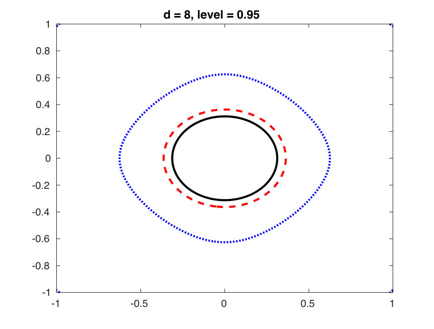 Figure 1
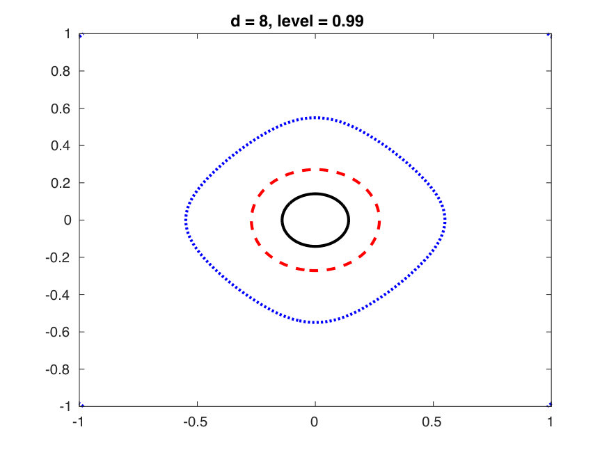 Figure 2
| a =1.4 | 5.71 | 3.55 | 5.38 | 3.27 |
| a= 1.3 | 5.38 | 3.41 | 5.04 | 3.21 |
| a= 1.2 | 5.02 | 3.31 | 4.70 | 3.18 |
| a= 1.1 | 4.56 | 3.25 | 4.32 | 3.16 |
| a= 1.0 | 3.91 | 3.20 | 3.87 | 3.15 |
| d=4 | d=4 (Stokes) | d=8 | d=8 (Stokes) | |
| 13% | 3.8% | 6.3% | 0.7% | |
| 16.6% | 2.1% | 9.8% | 0.2% | |
| 26.6% | 6.5% | 18.5% | 1.0% | |
| 44.7% | 22.7% | 31.2% | 8.2% |
| d=7 | d=7 (Stokes) | d=10 | d=10 (Stokes) | |
| 2.3% | 0.4% | 2.3% | 0.2% | |
| 30% | 10% | 26% | 5.5% | |
| 52% | 24% | 46% | 16% |
Peer Reviews
No public reviews on file for this paper yet. If you reviewed it on a platform where reviews are public (OpenReview, ICLR, NeurIPS, ICML), you can paste yours below so the community can read it here.
Videos
No videos yet. Explain this paper in a talk, walkthrough, or lecture? Add one.
Taxonomy
TopicsRisk and Portfolio Optimization · Probabilistic and Robust Engineering Design · Numerical Methods and Algorithms
Representation of chance-constraints with strong
asymptotic guarantees
Jean B. Lasserre1 *This work was supported by the European Research Council (ERC) via an ERC-Advanced Grant for the # 666981 project TAMING. The author is very grateful to Tillmann Weisser for his help in the numerical experiments.1Jean B Lasserre is senior researcher at LAAS-CNRS and the Institute of Mathematics, University of Toulouse, France. [email protected]
Abstract
Given , a probability measure on and a semi-algebraic set , we consider the feasible set associated with a chance-constraint. We provide a sequence of outer approximations , , where is a polynomial of degree whose vector of coefficients is an optimal solution of a semidefinite program. The size of the latter increases with the degree . We also obtain the strong and highly desirable asymptotic guarantee that as increases, where is the Lebesgue measure on . Inner approximations with same guarantees are also obtained.
Index Terms:
Probabilistic constraints; chance-constraints; semidefinite programming; semidefinite relaxations
I Introduction
We consider the following general framework for decision under uncertainty : Let be a decision variable while is a disturbance (or noise) parameter whose distribution (with support ) is known, i.e., its list of moments , , is available in closed form or numerically.
Both and are linked by constraints of the form , where
[TABLE]
for some polynomials , that is, is a basic semi-algebraic set.
Next, for each fixed , let be the (possibly empty) set defined by:
[TABLE]
Let be fixed. The goal of this paper is to provide tight approximations of the set
[TABLE]
in the form:
[TABLE]
where is a polynomial of degree at most .
Such approximations are particularly useful for optimization and control problems with chance-constraints; for instance problems of the form:
[TABLE]
Indeed one then replaces problem (5) with
[TABLE]
where the uncertain parameter has disappeared. So if is a basic semi-algebraic set then (6) is a standard polynomial optimization problem. Of course the resulting decision problem (6) may still be hard to solve because the sets and are not convex in general. But this may be the price to pay for avoiding a too conservative formulation of the problem. The interested reader is referred to Henrion [3], Prékopa [14] and Shapiro [15] for a general overview of chance constraints in optimization and to Calafiore and Dabbene [2], Jasour et al. [7] and Li et al. [13] in control (and the references therein).
However, in the formulation (6) one has got rid of the disturbance parameter , and so one may apply the arsenal of Non Linear Programming algorithms to get a local minimizer of (6). If is not too large or if some sparsity is present in problem (6) one may even run a hierarchy of semidefinite relaxations to approximate its global optimal value. For the latter approach the interested reader is referred to [10] and for a discussion on this approach to various control problems with chance constraints we refer to the recent paper of Jasour et al. [7] and the references therein.
In Jasour et al. [7] the authors have considered some control problems with chance constraints. They have provided an elegant formulation and a numerical scheme for solving the related problem of computing
[TABLE]
This problem is posed as an infinite-dimensional LP problem in an appropriate space of measures, that is, a Generalized Moment Problem (GMP) as described in Lasserre [10]. Then to obtain they solve a hierarchy of semidefinite relaxations, which is the moment-SOS approach for solving the GMP. This GMP formulation has the particular and typical feature of including a constraint of domination between two measures and . Such domination constraints are particularly powerful and have been already used in a variety of different contexts. See for instance Henrion et al. [5] for approximating the Lebesgue volume of a compact semi-algebraic set, Lasserre [12] for computing Gaussian measures of semi-algebraic set, Lasserre [11] for “approximating” the Lebesgue decomposition of a measure with respect to another one. It has been used by Henrion and Korda [6] for approximating regions of attraction, by Korda et al. [9] for approximating maximum controlled invariant sets, and more recently in Jasour and Lagoa [8] for a unifying treatment of some control problems.
Contribution
The approach that we propose for determining the set defined in (4) is very similar in spirit to that in [5] and [7] and can be viewed as an additional illustration of the versatility of the GMP and the moment-SOS approach in control related problems. Indeed we also define an infinite-dimensional LP problem in an appropriate space of measures and a sequence of semidefinite relaxations of , whose associated monotone sequence of optimal values converges to the optimal value of . An optimal solution of the dual of allows to obtain a polynomial of degree whose super-level set is precisely the desired approximation of in (4); in fact the sets provide a sequence of outer approximations of . We also provide the strong asymptotic guarantee that
[TABLE]
where is the Lebesgue measure on , which to the best of our knowledge is the first result of this kind at this level of generality. (The same methodology applied to chance-constraints of the form would provide a sequence of inner approximations of the set .)
Another contribution is to include a technique to accelerate the convergence which otherwise can be too slow. This technique is different from the one used in [5] for the related problem of computing the volume of a semi-algebraic set, and has the nice feature or preserving the monotonicity of the convergence of . It can be applied whenever is the Lebesgue measure on or or for some homogeneous nonnegative polynomial .
At last but not least, in principle we can also treat the case where the support of and the set are not compact, which includes the important case where is the normal distribution. We briefly explain what are the (technical) arguments which allow to extend the method to the non compact case.
Of course this methodology is computationally expensive and so far limited to relatively small size problems (but after all the problem is very hard). An interesting issue not discussed here is to investigate whether sparsity patterns can be exploited to handle problems with larger size.
II Notation, definitions and preliminary results
II-A Notation and definitions
Let be the ring of polynomials in the variables and let be the vector space of polynomials of degree at most (whose dimension is ). For every , let , and let , , be the vector of monomials of the canonical basis of . A polynomial is written
[TABLE]
Given a closed set , denote by the space of finite Borel measures on and by the convex cone of polynomials that are nonnegative on .
Moment matrix. Given a sequence , let be the linear (Riesz) functional
[TABLE]
Given and , the moment matrix associated with , is the real symmetric matrix with rows and columns indexed in and with entries
[TABLE]
Localizing matrix. Given a sequence , and a polynomial , the localizing moment matrix associated with and , is the real symmetric matrix with rows and columns indexed in and with entries
[TABLE]
II-B The volume of a compact semi-algebraic set
In this section we recall how to approximate as closely as desired the Lebesgue volume of a compact semi-algebraic set . It will be the building block of the methodology to approximate the set in (I).
Let be a box and let be the Lebesgue measure on . Let , assumed to be compact. For convenience and with no loss of generality we may and will assume that for some .
Theorem II.1** ([5])**
Let and with nonempty interior. Then
[TABLE]
and is the unique optimal solution.
Problem (7) is an infinite-dimensional LP with dual
[TABLE]
where is the space of continuous functions on . That (8) and (9) have same optimal value follows from compactness of and Stone-Weierstrass Theorem. Next, as shown in [5], there is no duality gap, i.e., .
II-C Semidefinite relaxations
Let , . To approximate one solves the hierarchy of semidefinite programs, indexed by :
[TABLE]
Interpretation.
Ideally, the variables (resp. ) of (10) should be viewed as “moments” of the measure (resp. the measure ) in (7) (and so ); the constraints (resp. ) are precisely necessary conditions for the above statement to be true111As , in principle one should also impose , , for all , to ensure that is supported on . However as for all , in the limit as , one has and so . (and which become sufficient as ).
The sequence is monotone non increasing and as . However the convergence is rather slow and in [5] the authors have proposed to replace the criterion by where is a polynomial that is nonnegative on and vanishes on the boundary of . If one denotes by an optimal solution of (10) then and as . The convergence is much faster but is not monotone anymore, which can be annoying because we do not obtain a decreasing sequence of upper bounds on as was the case with (10). For more details the interested reader is referred to [5].
II-D Stokes can help
This is why we propose another technique to accelerate the convergence in (10) while maintaining its monotonicity. So let be such that for all (but is not required to be nonnegative on ). Then by Stokes’ theorem (with vector field , , ), for each :
[TABLE]
and so the optimal solution of Theorem II.1 must satisfy
[TABLE]
Therefore in (10) we may impose the additional moment constraints
[TABLE]
To appreciate the impact of such additional constraints on the convergence , consider the simple example with and , let so that . For different values of and , results are displayed in Table I.
Remark II.2
Theorem II.1 is valid for any measure and not only the Lebesgue measure . On the other hand, additional Stokes constraints similar to (11) (but now with vector field and polynomial below) are valid provided that or for some homogeneous polynomial . Then with ,
[TABLE]
III Main Result
After the preliminary results of §II, we are now in position to state our main result. Let be the distribution of the noise parameter , and let be the Lebesgue measure on . The notation denotes the product measure on , that is,
[TABLE]
With as in (1), and for every , let be as in (2) (possibly empty). Consider the infinite dimensional LP:
[TABLE]
Theorem III.1
The unique optimal solution of (12) is
[TABLE]
and the optimal value of (12) satisfies
[TABLE]
Proof:
That follows from Theorem II.1 (with instead of in Theorem II.1). By Fubini-Tonelli’s Theorem (see Ash [1][Theorem 2.6.6, p. 103])
[TABLE]
[TABLE]
∎
Semidefinite relaxations
Let for all . As we did for (10) in §II, let and , , and relax (12) to the following hierarchy of semidefinite programs, indexed by :
[TABLE]
and of course for all . The dual of (14) is the semidefinite program:
[TABLE]
Again as is compact, for technical reasons (but with no loss of generality) we may and will assume that in the definition (1) of , for some .
Theorem III.2
Let and be with nonempty interior. There is no duality gap between (14) and its dual (15), i.e., for all . In addition (15) has an optimal solution such that
[TABLE]
Define to be:
[TABLE]
Then for all and
[TABLE]
as .
Proof:
That is because Slater’s condition holds for (14). Indeed let be the moments of in Theorem III.1 and be the moments of (on ). Then as has nonempty interior, and for all . Similarly as has nonempty interior, . Moreover since the optimal value is finite for all this implies that (15) has an optimal solution . Therefore:
[TABLE]
where follows from on . Finally the convergence follows from Theorem II.1. ∎
Then as on , the sets , , form a sequence of outer approximations of the set . In fact more can be said.
Corollary III.3
Let be as in Theorem III.2. Then the function is nonnegative on and converges to [math] in . In particular in -measure222A sequence of functions on a measure space converges in measure to if for all , as . The sequence converges almost-uniformly to if to every there exists a set such that and uniformly in ., and -almost uniformly for some subsequence .
Proof:
As as ,
[TABLE]
whence the convergence to [math] in . Then convergence in -measure, and -almost sure convergence for a subsequence follow from standard results from Real Analysis. See e.g. Ash [1, Theorem 2.5.1]. ∎
As we next see, the convergence in -measure established in Corollary III.3 will be useful to obtain strong asymptotic guarantees.
III-A Strong asymptotic guarantees
We here investigate asymptotic properties of the sequence of sets , as .
Corollary III.4
With as in (I), let where is as in Theorem III.2, . Then:
[TABLE]
Proof:
Observe that
[TABLE]
and therefore
[TABLE]
Next, for each , write
[TABLE]
By the convergence in -measure as , and so
[TABLE]
This implies
[TABLE]
which in turn yields the desired result (16). ∎
III-B Inner Approximations
In the previous section we have provided a converging sequence of outer approximations of . Clearly, letting , the same methodology now applied to a chance constraint of the form
[TABLE]
would provide a converging sequence of inner approximations of the set . To do so, (i) write as a finite union of basic semi-algebraic sets (whose measure of their overlaps is zero), (iii) apply the above methodology to each , and then (ii) sum-up the results.
III-C Accelerating convergence
As we already have seen in Section II-D for the semidefinite program (10), as the convergence of the optimal value of (14) can also be slow due to the Gibb’s phenomenon333The Gibbs’ phenomenon appears at a jump discontinuity when one approximates a piecewise function with a continuous function, e.g. by its Fourier series. that appears in the dual (15) when approximating the indicator function by a polynomial.
So assume that is the Lebesgue measure on where for instance , scaled to be a probability measure (but the same idea works if , or if for s ome homogeneous polynomial ). Then again we propose to include additional constraints on the moments and in (14) coming from additional properties of the optimal solution and of (12). Again these additional properties are coming from Stokes’ formula but now for integrals on (resp. ), then integrated over .
Let be the polynomials and of respective degree , . For each fixed , the polynomial (resp. ) vanishes on the boundary of (resp. of ). Therefore for each , Stokes’ Theorem (applied with vector fields (where ), ), states:
[TABLE]
[TABLE]
So let of degree , , be:
[TABLE]
for all , . Then for each :
[TABLE]
[TABLE]
Equivalently, in view of what are in Theorem III.1,
[TABLE]
Therefore in (14) we may include the additional moments constraints , and , for all such that and respectively.
III-D The non-compact case
In some applications the noise is assumed to follow a normal distribution on . Therefore is not compact anymore and the machinery used in [5] cannot be applied directly. However the normal distribution satisfies the important Carleman’s property. That is, let be the Riesz functional associated with , i.e., for all . Then
[TABLE]
In particular is moment determinate, that is, is completely determined by its moments. These two properties have been used extensively in e.g. Lasserre [11] and also in [12], precisely to show that with not necessarily compact, one may still approximate its Gaussian measure as closely as desired. Again one solves (7) via the same hierarchy of semidefinite relaxations (10) (but now with instead of ). For more details the interested reader is referred to Lasserre [11, 12].
In view of the above (technical) remarks, one may then extend the machinery described in §III to the case where , is the Gaussian measure, and () is not necessarily compact. A version of Stokes’ Theorem for non compact sets is even described in [12] to accelerate the convergence of the semidefinite relaxations (10) (with instead of ). It can be used to accelerate the convergence of the semidefinite relaxations (14), exactly as we do in §III-C for the compact case.
III-E Numerical examples
For illustration purposes we have considered simple small dimensional examples for which the function has a closed form expression, so that we can compare the set with its approximations , , obtained in Corollary III.4 (with and without using Stokes constraints).
Example III.5
, and . and are the Lebesgue measure. In this case . In Table II we display the relative error for different values of and , with and without Stokes constraints. The results indicate that adding Stokes constraints help a lot. With relatively few moments one obtains good approximations.
Example III.6
, and . and are the Lebesgue measure on and respectively. In this case, when , the set is the union of two disconnected intervals, hence more difficult to approximate. As in Example III.5, in Table III we display the relative error for different values of and , with and without Stokes constraints. Again, the results indicate that adding the Stokes constraints help a lot. With relatively few moments one obtains good approximations. For instance, while one obtains with Stokes and the larger set without Stokes constraints.
Example III.7
, and . and are the Lebesgue measure on and respectively. For this two-dimensional example (in ) we have plotted the boundary of the set (inner approximate circle, solid line in black). The curve in the middle (red dashed line) (resp. outer, blued dashed line) is the boundary of the approximation computed with Stokes constraints (resp. without Stokes constraints). For and the results are plotted in Fig. 1 and in Fig. 2 for and .
IV CONCLUSION
We have presented a systematic numerical scheme to provide an sequence of outer and inner approximations of the feasible set associated with chance constraints of the form . Each outer and inner approximation is the [math]-super level set of some polynomial whose coefficients are computed via solving a certain semidefinite program. As increases , a nice and highly desirable asymptotic property. Of course this methodology is computationally expensive and in its present form limited to problems of small size. But we hope it can pave the way to define efficient heuristics. Also checking whether this methodology can accommodate potential sparsity patterns present in larger size problems, is a topic of further investigation.
The reference list from the paper itself. Each links out to its DOI / PubMed record.
- 1[1] R. Ash, Real Analysis and Probability, Academic Press Inc., Boston, USA, 1972
- 2[2] G. Calafiore, F. Dabbene, Probabilistic and Randomized Methods for Design under Uncertainty, G. Calafiore and F. Dabbene (Eds.), Springer, 2006.
- 3[3] R. Henrion, Structural Properties of Linear Probabilistic Constraints, Optimization 56, pp. 425–440, 2007.
- 4[4] P. Kall, S.W. Wallace, Stochastic Programming , Wiley, 1994.
- 5[5] D. Henrion, J. B. Lasserre, C. Savorgnan, Approximate volume and integration for basic semialgebraic sets, SIAM Review 51, No. 4, pp. 722-743, 2009.
- 6[6] D. Henrion, M. Korda, Convex computation of the region of attraction of polynomial control systems. IEEE Trans. Aut. Control 59, No 2, pp. 297–312, 2014.
- 7[7] A. M. Jasour, N.S. Aybat, C. M. Lagoa, Semidefinite programming for chance constrained optimization over semi-algebraic sets, SIAM J. Optim. 25, No 3, pp. 1411–1440, 2015
- 8[8] A. Jasour, C. Lagoa, Convex constrained semialgebraic volume optimization: Application in systems and control, 2017, ar Xiv:1701.08910