Quantum Thermal Machine as a Thermometer
Patrick P. Hofer, Jonatan Bohr Brask, Mart\'i Perarnau-Llobet, and, Nicolas Brunner

TL;DR
This paper introduces a quantum thermal machine-based thermometer capable of precise low-temperature measurements down to 15 mK, leveraging quantum Fisher information for near-optimal performance in complex systems.
Contribution
It proposes a novel thermometry method using quantum thermal machines that works without detailed knowledge of coupling constants and is implementable with circuit QED technology.
Findings
Achieves thermometry down to ~15 mK with realistic parameters.
Operates effectively without precise thermalization between components.
Close to the theoretical limit set by quantum Fisher information.
Abstract
We propose the use of a quantum thermal machine for low-temperature thermometry. A hot thermal reservoir coupled to the machine allows for simultaneously cooling the sample while determining its temperature without knowing the model-dependent coupling constants. In its most simple form, the proposed scheme works for all thermal machines which perform at Otto efficiency and can reach Carnot efficiency. We consider a circuit QED implementation which allows for precise thermometry down to 15 mK with realistic parameters. Based on the quantum Fisher information, this is close to the optimal achievable performance. This implementation demonstrates that our proposal is particularly promising in systems where thermalization between different components of an experimental setup cannot be guaranteed.
Click any figure to enlarge with its caption.
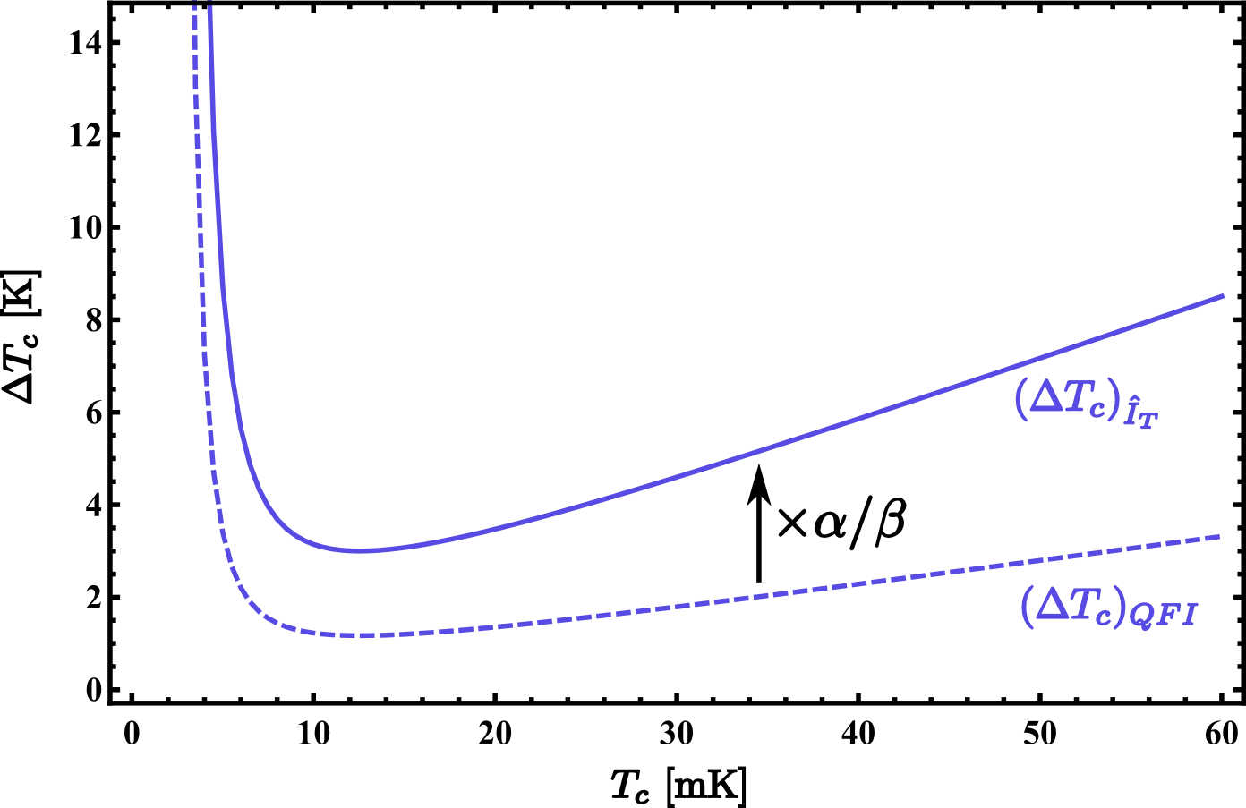 Figure 1
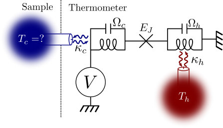 Figure 2
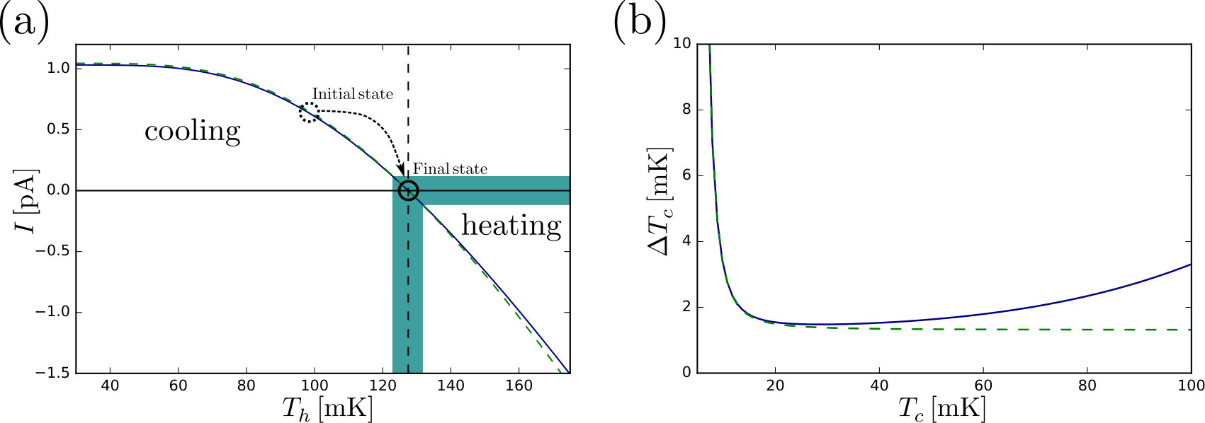 Figure 3
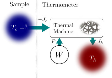 Figure 4
| GHZ | GHZ | GHz | GHz | pA | mK |
Peer Reviews
No public reviews on file for this paper yet. If you reviewed it on a platform where reviews are public (OpenReview, ICLR, NeurIPS, ICML), you can paste yours below so the community can read it here.
Videos
No videos yet. Explain this paper in a talk, walkthrough, or lecture? Add one.
Quantum Thermal Machine as a Thermometer
Patrick P. Hofer
Département de Physique Appliquée, Université de Genève, 1211 Genève, Switzerland
Jonatan Bohr Brask
Département de Physique Appliquée, Université de Genève, 1211 Genève, Switzerland
Martí Perarnau-Llobet
Max-Planck-Institut für Quantenoptik, Hans-Kopfermann-Str. 1, D-85748 Garching, Germany
ICFO-Institut de Ciencies Fotoniques, The Barcelona Institute of Science and Technology, 08860 Castelldefels, Barcelona, Spain
Nicolas Brunner
Département de Physique Appliquée, Université de Genève, 1211 Genève, Switzerland
Abstract
We propose the use of a quantum thermal machine for low-temperature thermometry. A hot thermal reservoir coupled to the machine allows for simultaneously cooling the sample while determining its temperature without knowing the model-dependent coupling constants. In its most simple form, the proposed scheme works for all thermal machines which perform at Otto efficiency and can reach Carnot efficiency. We consider a circuit QED implementation which allows for precise thermometry down to mK with realistic parameters. Based on the quantum Fisher information, this is close to the optimal achievable performance. This implementation demonstrates that our proposal is particularly promising in systems where thermalization between different components of an experimental setup cannot be guaranteed.
Introduction.— Accurate sensing and measuring of temperature is of crucial importance throughout natural science and technology. Increased capabilities of control and imaging on smaller and smaller scales have led to the need for precise thermometry down to millikelvin temperatures at sub-micron scales. Conventional techniques are not applicable in this regime, resulting in the development of a broad range of new methods over the last decade Carlos and Palacio (2016). Many of these employ probes which are so small that quantum effects become relevant in their design and sensing capabilities, e.g. quantum dots Walker et al. (2003); Seilmeier et al. (2014); Haupt et al. (2014), nitrogen-vacancy centers in diamond Toyli et al. (2013); Kucsko et al. (2013); Neumann et al. (2013), superconducting quantum interference devices Halbertal et al. (2016), and even biomolecules Donner et al. (2012). At the same time, the study of thermal processes in the quantum regime has recently seen increased interest fueled by tools developed in quantum information theory Goold et al. (2016); Vinjanampathy and Anders (2016). This approach has led to novel insights into the limitations of measuring cold temperatures posed by quantum theory Stace (2010); Marzolino and Braun (2013); Correa et al. (2015); Paris (2016); De Pasquale et al. (2016), showing that coherence can be beneficial for low temperature thermometry Stace (2010); Jevtic et al. (2015); Johnson et al. (2016); Martín-Martínez et al. (2013); Sabín et al. (2014).
In a standard approach to thermometry, a probe is brought into thermal contact with the sample and the system is allowed to equilibrate Haupt et al. (2014); Seilmeier et al. (2014). The temperature is then read out through some observable on the probe whose relation to the temperature is known. The measurement can possibly be improved by letting the probe interact with the sample for a finite time only, making use of the transient dynamics Guo et al. (2015); Jevtic et al. (2015), or by increasing the coupling strength between sample and probe Correa et al. (2016). Both of these approaches lead to a non-equilibrium state for the probe. Another approach to thermometry, which is employed to measure electronic temperatures, makes use of a voltage bias that creates an out-of-equilibrium situation. The temperature can then be determined through the current-voltage characteristics Giazotto et al. (2006); Iftikhar et al. (2016); Zgirski et al. (2017). We note that these strategies generally lead to unwanted heating of the sample.
In this letter, we connect thermometry to quantum thermal machines. Such machines are extensively studied to investigate fundamental as well as practical aspects of quantum thermodynamics Goold et al. (2016); Benenti et al. (2017); Kosloff and Levy (2014); Quan et al. (2007); Brunner et al. (2012). By construction, these machines constitute out-of-equilibrium systems including a temperature gradient. Here we consider a quantum refrigerator to simultaneously cool the sample and estimate its temperature. This way, the proposed thermometer does not induce any heating of the sample, even if it is at the coldest temperature that is experimentally available. Our proposal thus makes use of a thermal bias to create an out-of-equilibrium situation that is favorable for thermometry. This idea goes back to Thomson (Lord Kelvin), who considered the use of a Carnot engine to determine an absolute temperature scale Thomson (1848) (see also Ref. Geusic et al. (1967)). Note that albeit the thermal bias, the sample is assumed to remain in local equilibrium throughout the measurement.
The main idea is illustrated in Fig. 1. The sample to be measured is a thermal bath at a cold temperature . Through a small quantum system (the machine), the sample is coupled to another bath at a higher temperature and an external power source (which in principle could be provided by a third thermal bath Linden et al. (2010); Skrzypczyk et al. (2011); Hofer et al. (2016a); Mitchison et al. (2016)). Note that this setup can operate either as a refrigerator, with the power source driving a heat flow from the cold to the hot bath, or as a heat engine, where work is generated using a heat flow from the hot to the cold bath Levy and Kosloff (2012); Kosloff and Levy (2014); Mitchison et al. (2015); Silva et al. (2015); Brunner et al. (2014); Brask and Brunner (2015); Roulet et al. (2017). Since we are interested in determining , the whole setup, apart from the cold bath, should be considered as the thermometer. By operating the machine as a refrigerator, the sample will be cooled during the measurement of , avoiding any undesirable heating. Furthermore, by approaching the Carnot point, where the machine approaches reversibility, the need for knowledge of the coupling constants can be eliminated, just as for thermalizing thermometry. We note that some knowledge of the hot bath temperature is required for our scheme. However, the cold temperature can be determined with high precision even if the hot temperature measurement is noisy. Our scheme can thus be seen as a method to turn an uncertain measurement of warm temperatures into precise measurements of cold temperatures working similarly to a Wheatstone bridge, where resistors of known resistances are used to determine an unknown resistance.
The rest of this letter is structured as follows. After describing the working principle of the proposed thermometer in more detail, we discuss an implementation in a circuit QED architecture, which allows for precise thermometry of a microwave resonator down to mK using realistic parameters. Finally, we investigate the precision of the thermometer using the quantum Fisher information.
Scheme.— We now turn to a more detailed description of our thermometer. The thermal bias and the power source induce energy flows denoted by (heat flow into the cold bath), (heat flow into the hot bath), and (power consumption, see Fig. 1). The power consumed by the machine will in general be a function of the temperatures as well as the model-dependent parameters. Inverting this relationship, the cold temperature can be written as
[TABLE]
Here, might have a complicated dependence on the coupling constants or any other model dependent parameters. However, the relation simplifies for machines that perform at the Otto efficiency and exhibit a Carnot point mah (2009). When the machine is operated as a heat engine, the efficiency is defined as . The Otto efficiency is given by where , are frequencies that depend on the architecture of the machine (see Fig. 2). For thermal machines that exhibit a Carnot point, setting the frequencies and temperatures such that
[TABLE]
results in vanishing energy flows. Examples of thermal machines which operate at the Otto efficiency and exhibit a Carnot point are discussed in Refs. Kosloff (1984); Feldmann and Kosloff (2003); Quan et al. (2007); Niskanen et al. (2007); Henrich et al. (2007); Hofer et al. (2016b); Campisi and Fazio (2016). We note that whenever the frequencies and temperatures are such that , the machine operates as a refrigerator. At the Carnot point, we find the simple relation
[TABLE]
implying that is independent of any coupling constants. Thomson proposed to use the above relation to determine an absolute temperature scale Thomson (1848). Here we use the same relation as a key ingredient in low temperature thermometry (see supplemental material for a discussion on imperfections that prevent Eq. (3) sup ). In order to reach the Carnot point, one can either modify the frequencies or the temperature associated with the thermometer. Here we focus on the case where the frequencies remain fixed but one has some control over . The cold temperature can then be determined using the following strategy (see Fig. 3)
Initiate the machine to act as a refrigerator, i.e. , and monitor 2. 2.
Increase until is reached 3. 3.
Measure 4. 4.
Determine using Eq. (3)
In this scheme, two quantities are measured to determine : The power consumption and the hot temperature . Both of these measurements are accompanied by errors, and . Simple error propagation yields (assuming independent errors)
[TABLE]
The error thus depends on the derivatives of which generally depend on model-specific parameters. Note however that implying that the error induced by the measurement of only depends on the frequencies. Any uncertainty in the measurement of can thus be compensated by increasing the ratio and thus does not represent a fundamental limit.
Circuit QED implementation.— We now turn to an implementation of these ideas, considering the heat engine proposed in Ref. Hofer et al. (2016b) and sketched in Fig. 2. In this machine, the quantum system consists of two -oscillators with frequencies and coupled to each other through a Josephson junction. Such a system has recently been implemented experimentally, investigating the emission of non-classical radiation Westig et al. (2017). See also Refs. Holst et al. (1994); Basset et al. (2010); Hofheinz et al. (2011) for related experiments. Each oscillator is coupled individually to a heat bath, one of which is the sample at temperature , and the power source is provided by an external voltage bias . We note that a similar setup (without any temperature bias however) has been considered for thermometry in Ref. Saira et al. (2016). The Hamiltonian describing the system reads (in a rotating frame)
[TABLE]
where is the Josephson energy, annihilates a photon in the oscillator with frequency and the non-linear operators are defined as
[TABLE]
with denoting the generalized Laguerre polynomials and where we defined the Fock states . We note that Eq. (5) is derived using a rotating wave approximation which holds under the resonance condition (for details, see Ref. Hofer et al. (2016b))
[TABLE]
The evolution of the system in contact with the thermal baths is captured by a local Lindblad master equation
[TABLE]
where we defined , denotes the energy damping rate associated with the bath , and the corresponding occupation number. In accordance with existing theory Gramich et al. (2013) and experiment Hofheinz et al. (2011), we neglect voltage fluctuations arising from a low-frequency environment. We note that the local master equation, Eq. (8), was recently shown to capture the thermodynamics of the considered heat engine very well Hofer et al. (2017); González et al. (2017). Alternatively one may also consider a master equation based on a Floquet formalism, see Refs. Alicki et al. (2006); Levy et al. (2012); Szczygielski et al. (2013).
The power consumption of the machine is , where is the (dc) electrical current with the current operator
[TABLE]
and the critical current. The mean heat currents are defined as
[TABLE]
All averages are taken with respect to the steady-state solution of Eq. (8). For a more detailed discussion on the working principle of the heat engine and the involved approximations, we refer the reader to Ref. Hofer et al. (2016b). It can be shown that this machine does perform at the Otto efficiency and can reach the Carnot efficiency at vanishing power. Furthermore, a tunable hot temperature could be implemented by heating one of the -oscillators using a microwave antenna. Therefore, this circuit QED engine exhibits all the features required to perform thermometry as discussed above.
Fig. 3 (a) shows the electrical current as a function of the hot temperature and sketches the scheme for measuring . The error of the measurement is plotted in Fig. 3 (b), where the parameters (including the uncertainties) are given in Tab. 1. We find a precision of mK for temperatures down to mK. In accordance with Ref. Hofer et al. (2016b), we find good quantitative agreement with an approximate model obtained from Eq. (5) by replacing the non-linear operators by constants times the identity sup . This model can be solved analytically and is used below to estimate the performance of our scheme using the quantum Fisher information. We note that instead of the electrical current, one could also measure the heat currents to determine the Carnot point.
Throughout this paper, we consider the thermometer as a device to determine the temperature of the cold bath. However, in this particular implementation, the thermometer measures the temperature of the microwave mode with frequency (see supplemental material for a discussion where this temperature is not equal to the bath temperature sup ). In situations where thermalization between different components of an experimental setup is difficult to achieve, our proposal thus provides a promising route to determine the physically relevant temperature. Another possibility for measuring the temperature in the circuit is to perform shot noise thermometry, where a magnetic field needs to be applied to bring the junction to the normal state, possibly influencing the temperature. Such a measurement was performed in Ref. Hofheinz et al. (2011) to determine the temperature of a microwave resonator coupled to a Josephson junction. In general, the precision obtained in our proposal compares well with electronic out-of-equilibrium thermometry Iftikhar et al. (2016).
Quantum Fisher information.— As already mentioned, the measurement error resulting from the hot temperature measurement is not of a fundamental nature since we can in principle reduce it by increasing (note however that this implies an increase of at the Carnot point). In order to understand how well the current measurement is doing in terms of temperature estimation, we turn to the quantum Fisher information.
The steady-state solution of Eq. (8) defines a family of states as a function of (as well as all the other parameters in the setup). The quantum Fisher information (QFI) w.r.t is a measure of the sensitivity of the state to changes in this parameter Holevo (1982). Through the quantum Cramer-Rao bound, it provides a lower bound on the mean-squared error in estimating from any possible measurement Braunstein and Caves (1994). Specifically,
[TABLE]
where is the QFI w.r.t. and is the number of independent repetitions of the experiment. The bound is relevant (and can be saturated) in the local estimation regime, where the prior on the estimated parameter is narrow and many repetitions are performed. In the same regime, for measuring a specific observable , the attainable precision is given by the error propagation formula
[TABLE]
Hence, by substituting the current operator for and comparing and evaluated in the steady state at the Carnot point, we can get an idea of how close the current measurement is to being optimal. Note that this neglects any errors in other parameters as well as the fact that our strategy is based on continuous measurements rather than projective measurements considered in Eq. (12). Although we should thus not expect this calculation to give us the actual uncertainty obtained in an experiment, it does tell us whether the current is a good choice of observable for estimating .
To perform the comparison, we first need to find the steady-state solution of Eq. (8). This can be done analytically for the approximate model discussed in the supplemental material sup yielding
[TABLE]
and
[TABLE]
where the parameters and depend on the coupling constants and are given in the supplemental material sup . We see that the current-measurement precision and the optimal precision from the QFI have exactly the same functional behavior with temperature and energy, but depend differently on the coupling constants. For any choice of couplings, such that . Both expressions are plotted in Fig. 4. The reason that the current operator is a good observable for determining is ultimately due to the fact that the current is very sensitive to the occupation number in the oscillators. Although the occupation numbers depend only very weakly on temperature at sufficiently low temperatures, measuring occupation numbers is in many scenarios still the optimal choice Campbell et al. (2017).
The smallest possible value of is , attained for (where is the interaction strength in the approximate model). For the parameters in Tab. 1, , and so the current measurement is close to its best performance in this regime. Furthermore, , hence it is also not far from the optimal precision obtainable by any possible measurement. The smallest possible value of is , however it is attained in the weak coupling limit , where no information about can be extracted and both and diverge. In the opposite limit where the hot reservoir is disconnected, , we have while reaches its minimal value. This reflects the fact that the current vanishes if the system is coupled to a single bath only, while even if there is no coupling to the hot bath, the steady state of the system still contains information about .
Conclusion.— In conclusion, we investigated the use of thermal machines as thermometers. The non-equilibrium nature of the steady state in these systems allows for simultaneously cooling the cold bath while determining its temperature. Furthermore, our scheme only requires the measurement of the power consumption and the hot temperature, both of which do not require any projective measurements on the quantum system which are difficult to implement. For realistic parameters, an implementation in circuit QED allows for precise thermometry ( mK) of a microwave resonator mode down to small temperatures (mK). While lower values have been reported (see e.g. Ref. Iftikhar et al. (2016) where precise thermometry down to mK has been reported) our scheme is of particular interest when thermalization between different components of an experimental setup cannot be guaranteed and heating of the sample has to be avoided. Our proposal can be readily adapted to other architectures.
Acknowledgements.— We acknowledge interesting discussions with L. Correa. P. H., J. B., and N. B. acknowledge the Swiss National Science Foundation (starting Grant DIAQ, Grant No. 200021_169002, and QSIT). M. P.-L. acknowledges the Alexander von Humboldt Foundation, the CELLEX-ICFO-MPQ research fellowships, the Spanish MINECO (Grants No. QIBEQI FIS2016-80773-P and No. SEV-2015-0522), and the Generalitat de Catalunya (Grants No. SGR875 and CERCA Programme).
I Approximate model
Here we consider the approximate model that is obtained from the master equation in the main text by the replacement , leading to the Hamiltonian and current operator
[TABLE]
where is treated as a fitting parameter. Such a model has first been investigated as a heat engine in Ref. Kosloff (1984). An analogous engine that is based on coupled qubits instead of harmonic oscillators was introduced in Ref. Brunner et al. (2012). The time-evolution of the harmonic oscillators is described by the local Lindblad master equation
[TABLE]
with
[TABLE]
and the Bose-Einstein distribution
[TABLE]
As usual, differential equations for averages of operators are obtained by
[TABLE]
Here we are interested in steady state values, where . For the mean current, this yields
[TABLE]
which is plotted in Fig. 3 (a). The uncertainty in the temperature measurement plotted in Fig. 3 (b) is obtained using
[TABLE]
and
[TABLE]
which yields the error
[TABLE]
I.1 Steady-state solution
The steady state solution of the master equation in Eq. (S2) is Gaussian because the equation is bi-linear in creation and annihilation operators. It is therefore completely characterised by the first and second order moments of the quadrature operators
[TABLE]
Furthermore, since no term in the master equation induces displacements, the state is centred in phase space, , and is thus determined by the second moments alone.
We note that because the evolution is not unitary, it is not possible to determine the second moments simply by solving the equations of motions for the quadrature operators (working in the Heisenberg picture). While for unitary evolution, the time evolution of a product of operators is equal to the product of the time-evolved operators – e.g. – this is not true in general. Hence, we need to derive the equations of motion for each of the second moments separately. We consider the 10 second moments , , , , , , , , , (the remaining six are determined by the commutation relations). From (S2), we find
[TABLE]
The steady state is found by setting all the derivatives to zero. We then get
[TABLE]
We note that for this is indeed a product of thermal states at temperatures and as expected. Also note that at the Carnot point we have , which also results in a product of thermal states.
II Computing the Fisher information
From the first and second moments of the quadratures – i.e. from the covariance matrix, and the displacement vector (if the latter is non-zero) – it is possible to compute the QFI, with respect to a given parameter of interest (in our case this is the cold bath temperature ). Various works have considered this problem, e.g. Monras (2013); Jiang (2014); Šafránek and Fuentes (2016); Sparaciari et al. (2016). Here, we will follow the method of Sparaciari et al. (2016).
We define a vector of the quadratures (note that this ordering is not the same as in Sparaciari et al. (2016), nevertheless their method still applies, see also Jiang (2014)). We restrict ourselves to the case where the first moments vanish, and define the covariance matrix as
[TABLE]
The canonical commutation relations are given by , where the symplectic matrix with this ordering of the is
[TABLE]
To compute the quantum Fisher information following (Sparaciari et al., 2016), one needs to find a symplectic diagonalisation of the covariance matrix. That is, one needs to find a transformation such that
[TABLE]
and
[TABLE]
where is diagonal. One can then proceed to define the matrix by
[TABLE]
where the dot denotes derivation with respect to , and are the eigenvalues of . One further defines , and the QFI is finally given by
[TABLE]
The symplectic diagonalisation is the most involved step of computing the QFI. For the steady-state solution in Eqs. (S12)
[TABLE]
where
[TABLE]
and
[TABLE]
Denoting the normalized eigenvectors of as row vectors by , , a symplectic transformation diagonalizing can be constructed as
[TABLE]
where Re and Im denote real and imaginary parts respectively. One finds that
[TABLE]
with
[TABLE]
From Eqs. (S17) and (S18), and by using that close to the Carnot point
[TABLE]
the expression for the QFI at the Carnot point can be found by taking the limit and reads
[TABLE]
The parameter in the main text thus reads
[TABLE]
III Computing the uncertainty from a current measurement
We aim to use Eq. (12) for the simple model given in Eq. (S1) in the steady state. The mean current and its derivative with respect to are given in Eqs. (S6) and (S8) respectively. The variance reads
[TABLE]
which simplifies to
[TABLE]
at the Carnot point where we have . Hence, we get that with a current measurement at the Carnot point
[TABLE]
which results in
[TABLE]
IV Heat leaks and spurious modes
Heat leaks, connecting the hot and the cold bath, as well as spurious modes which couple to the Cooper pairs can lead to an efficiency that deviates from the Otto efficiency, impeding the measurement of the cold temperature. Here we discuss these issues in detail, showing that they do not pose a major problem.
In the absence of heat leaks, the oscillators thermalize to the bath temperatures whenever the back-action of the Cooper pair current can be neglected (this is the case at the Carnot point, or if the voltage is not at resonance , or if either or go to zero). The thermometer then measures the temperature of the cold bath as discussed in the main text. In the presence of heat leaks, the oscillators will not necessarily thermalize to the bath temperatures even when the back-action of the current can be neglected. Denoting the temperatures of the oscillators in the absence of a Cooper pair current as , the corresponding occupation numbers read . Importantly, the power consumption of the engine will go to zero when which implies . If the hot temperature measurement required for our proposal measures , our thermometer will thus determine . Since this is the steady-state temperature of the oscillator with frequency (in the absence of a current), this is arguably the temperature of interest. If the hot temperature measurement still measures the bath temperature , any difference can be accounted for in the error . We note that only heat leaks that involve the oscillator degrees of freedom will lead to . Any additional heat currents in or out of the baths that do not involve the oscillator degrees of freedom do not change the results of the main text in any way. This is important since in practice the baths will be stabilized with heat flows that are not taken into account in the analysis.
Spurious modes which have a finite density of states at the Josephson frequency lead to a finite current (dissipating power) even when . This could in principle be detrimental to our thermometry scheme. However, by sweeping the voltage, the environment that couples to the Josephson junction can be characterized fairly well. Experiments suggest that spurious modes at the Josephson frequency can be avoided Hofheinz et al. (2011); Westig et al. (2017). Even if such modes are present, one can in principle determine if their presence is known. In this case, one can correct for the dissipative current.
The reference list from the paper itself. Each links out to its DOI / PubMed record.
- 1Carlos and Palacio (2016) L. D. Carlos and F. Palacio, eds., Thermometry at the Nanoscale (The Royal Society of Chemistry, 2016). · doi ↗
- 2Walker et al. (2003) G. W. Walker, V. C. Sundar, C. M. Rudzinski, A W. Wun, M G. Bawendi, and D G. Nocera, “Quantum-dot optical temperature probes,” Appl. Phys. Lett. 83 , 3555 (2003) . · doi ↗
- 3Seilmeier et al. (2014) F. Seilmeier, M. Hauck, E. Schubert, G. J. Schinner, S. E. Beavan, and A. Högele, “Optical thermometry of an electron reservoir coupled to a single quantum dot in the millikelvin range,” Phys. Rev. Applied 2 , 024002 (2014) . · doi ↗
- 4Haupt et al. (2014) F. Haupt, A. Imamoglu, and M. Kroner, “Single quantum dot as an optical thermometer for millikelvin temperatures,” Phys. Rev. Applied 2 , 024001 (2014) . · doi ↗
- 5Toyli et al. (2013) D. M. Toyli, C. F. de las Casas, D. J. Christle, V. V. Dobrovitski, and D. D. Awschalom, “Fluorescence thermometry enhanced by the quantum coherence of single spins in diamond,” Proc. Natl. Acad. Sci. U.S.A. 110 , 8417 (2013) . · doi ↗
- 6Kucsko et al. (2013) G. Kucsko, P. C. Maurer, N. Y. Yao, M. Kubo, H. J. Noh, P. K. Lo, H. Park, and M. D. Lukin, “Nanometre-scale thermometry in a living cell,” Nature 500 , 54 (2013) . · doi ↗
- 7Neumann et al. (2013) P. Neumann, I. Jakobi, F. Dolde, C. Burk, R. Reuter, G. Waldherr, J. Honert, T. Wolf, A. Brunner, J. H. Shim, D. Suter, H. Sumiya, J. Isoya, and J. Wrachtrup, “High-precision nanoscale temperature sensing using single defects in diamond,” Nano Lett. 13 , 2738 (2013) . · doi ↗
- 8Halbertal et al. (2016) D. Halbertal, J. Cuppens, M. Ben Shalom, L. Embon, N. Shadmi, Y. Anahory, H. R. Naren, J. Sarkar, A. Uri, Y. Ronen, Y. Myasoedov, L. S. Levitov, E. Joselevich, A. K. Geim, and E. Zeldov, “Nanoscale thermal imaging of dissipation in quantum systems,” Nature 539 , 407 (2016) . · doi ↗