The matter-ekpyrotic bounce scenario in Loop Quantum Cosmology
Jaume Haro, Jaume Amor\'os, Llibert Arest\'e Sal\'o

TL;DR
This paper analyzes a matter-ekpyrotic bounce scenario within Loop Quantum Cosmology, demonstrating its viability for producing a nearly scale-invariant power spectrum and successful reheating consistent with observational data.
Contribution
It provides a detailed dynamical systems analysis of the matter-ekpyrotic bounce in Loop Quantum Cosmology, including particle production and perturbation spectra.
Findings
Universe transitions from matter domination to ekpyrotic phase in contraction
Reheating occurs via production of heavy and massless particles
Perturbation spectra are nearly scale-invariant and compatible with PLANCK data
Abstract
We will perform a detailed study of the matter-ekpyrotic bouncing scenario in Loop Quantum Cosmology using the methods of the dynamical systems theory. We will show that when the background is driven by a single scalar field, at very late times, in the contracting phase, all orbits depict a matter dominated Universe, which evolves to an ekpyrotic phase. After the bounce the Universe enters in the expanding phase, where the orbits leave the ekpyrotic regime going to a kination (also named deflationary) regime. Moreover, this scenario supports the production of heavy massive particles conformally coupled with gravity, which reheats the universe at temperatures compatible with the nucleosynthesis bounds and also the production of massless particles non-conformally coupled with gravity leading to very high reheating temperatures but ensuring the nucleosynthesis success. Dealing with…
Click any figure to enlarge with its caption.
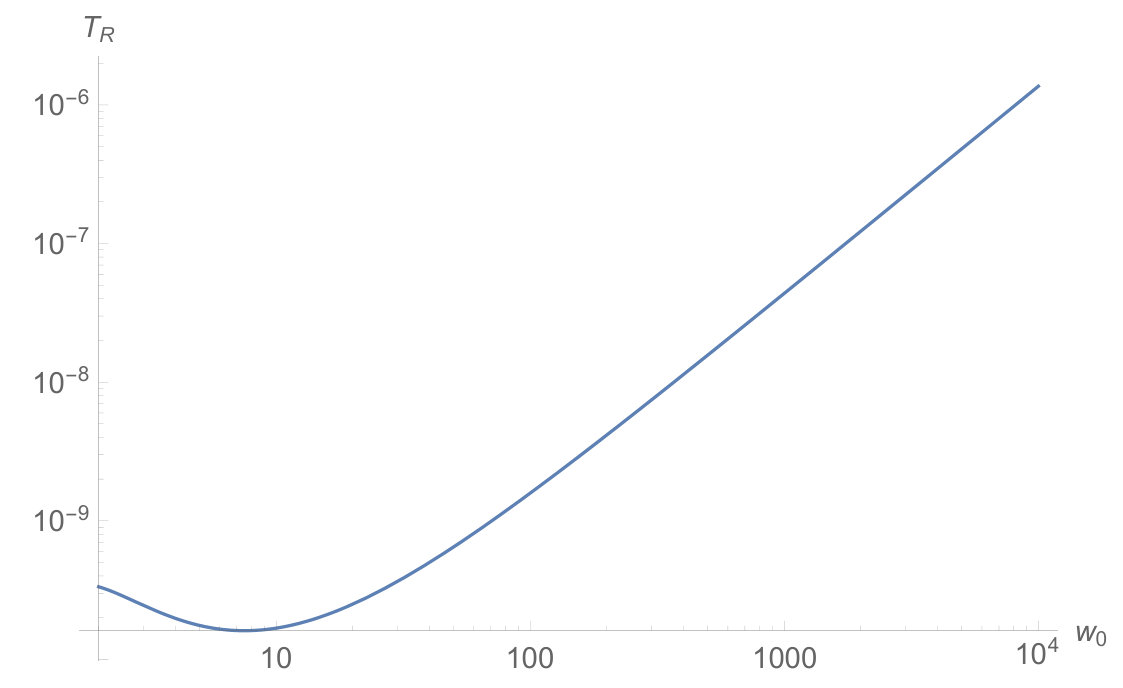 Figure 1
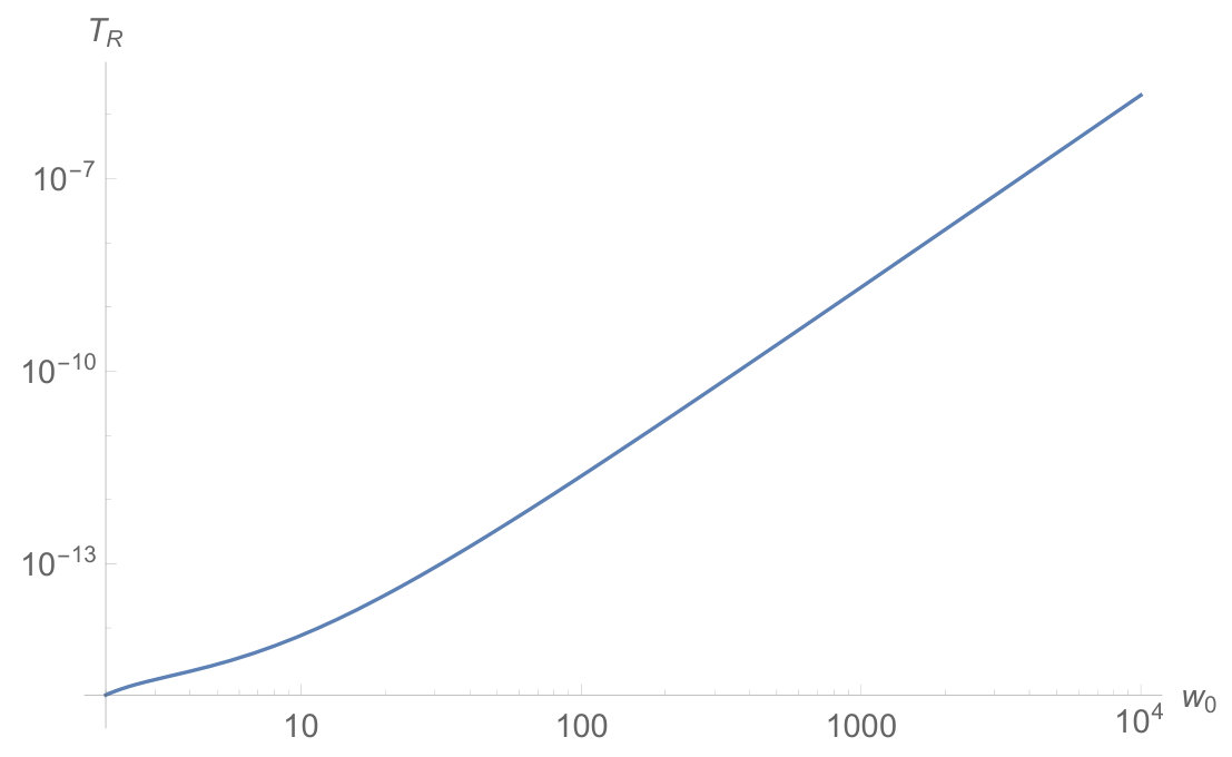 Figure 2
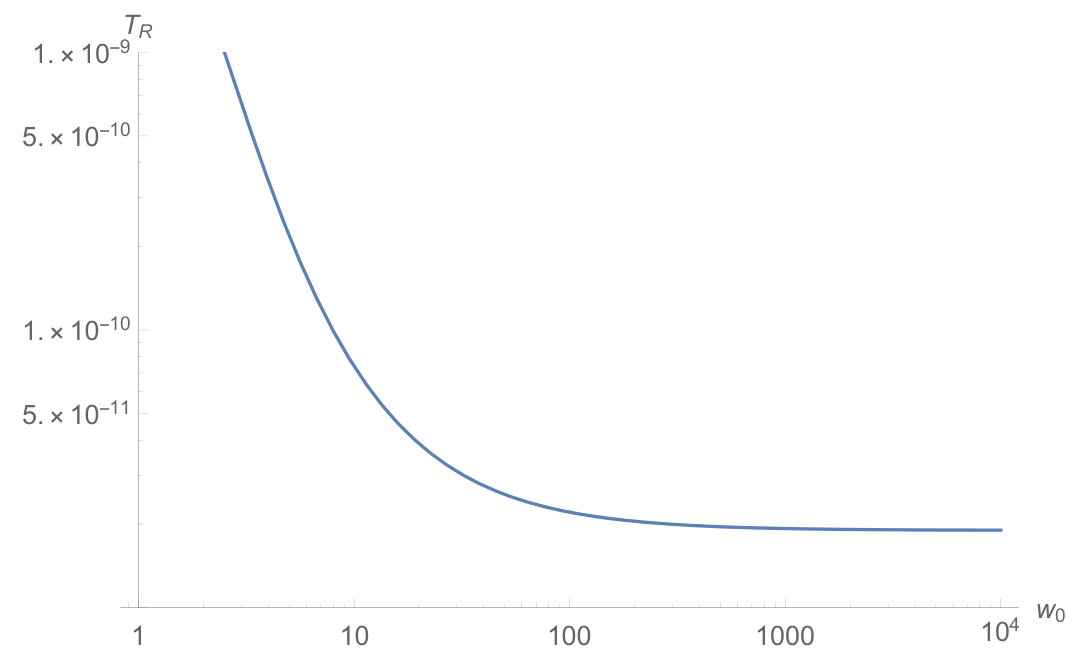 Figure 3
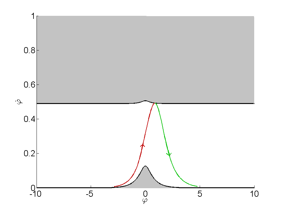 Figure 4
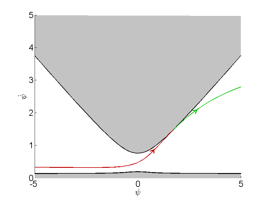 Figure 5
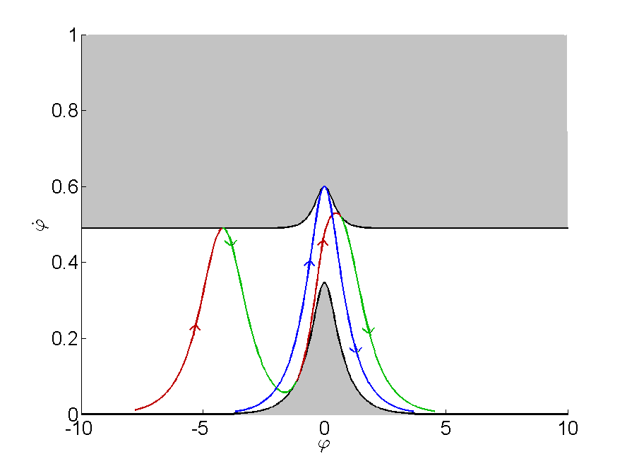 Figure 6
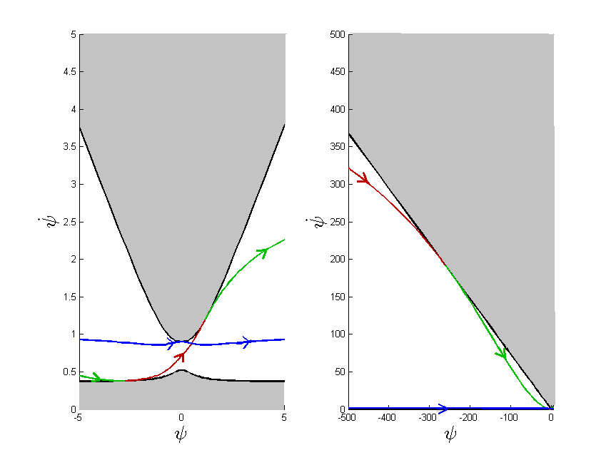 Figure 7
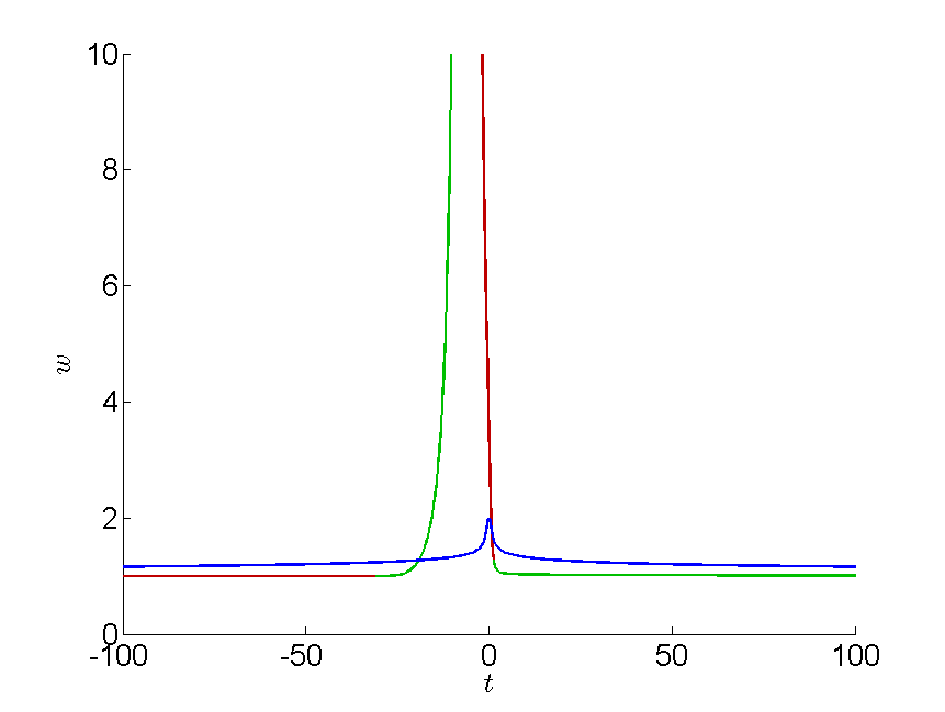 Figure 8
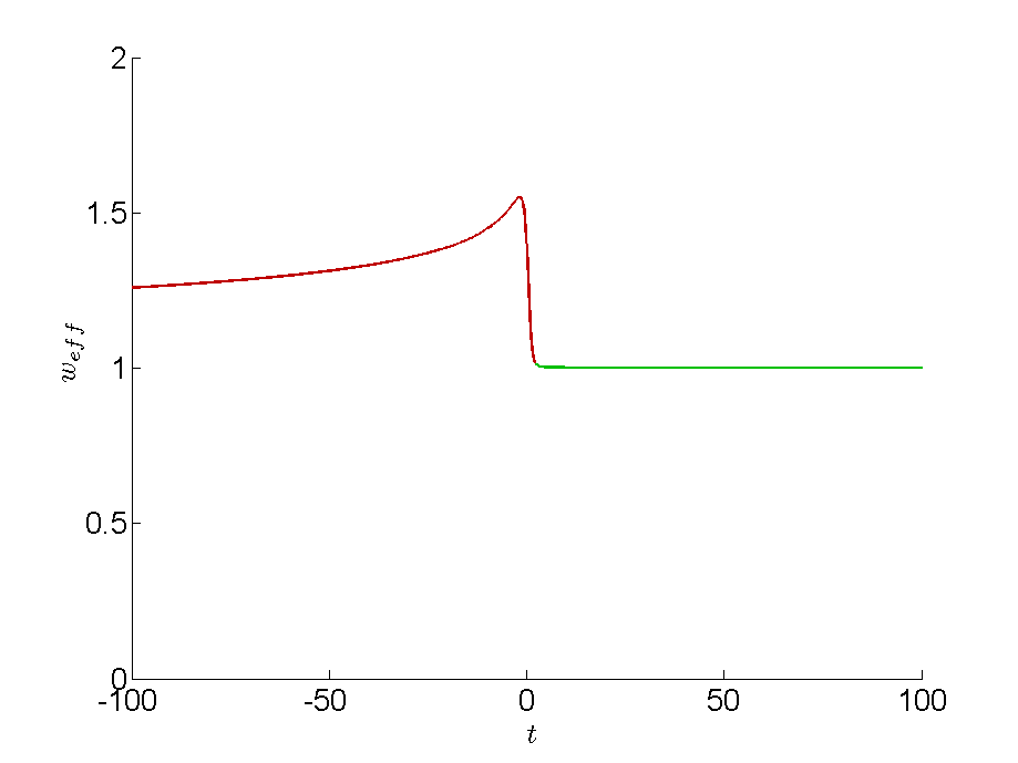 Figure 9
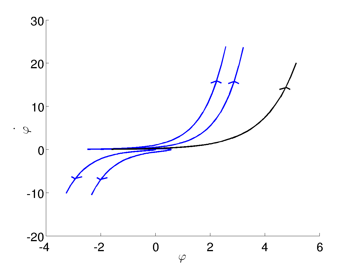 Figure 10
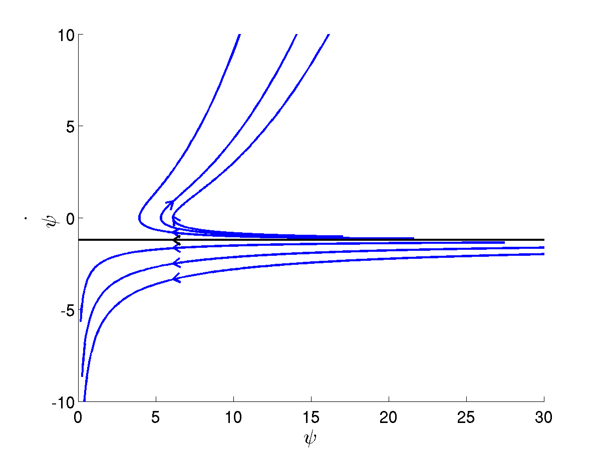 Figure 11
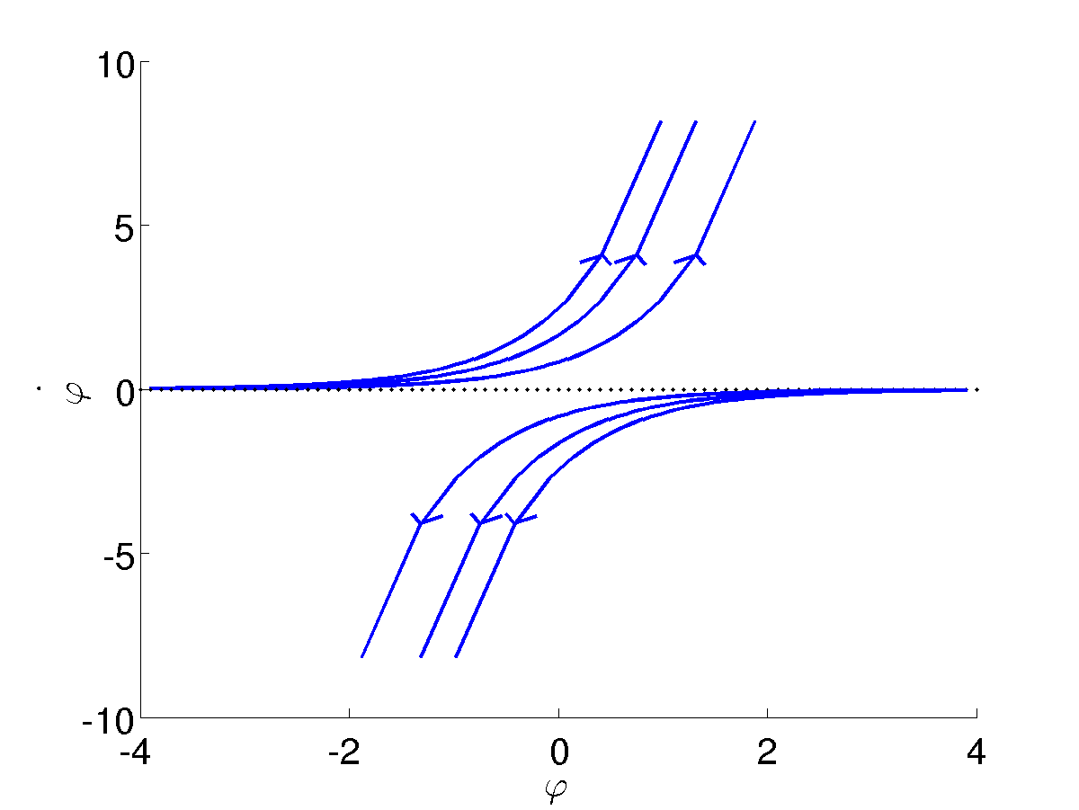 Figure 12
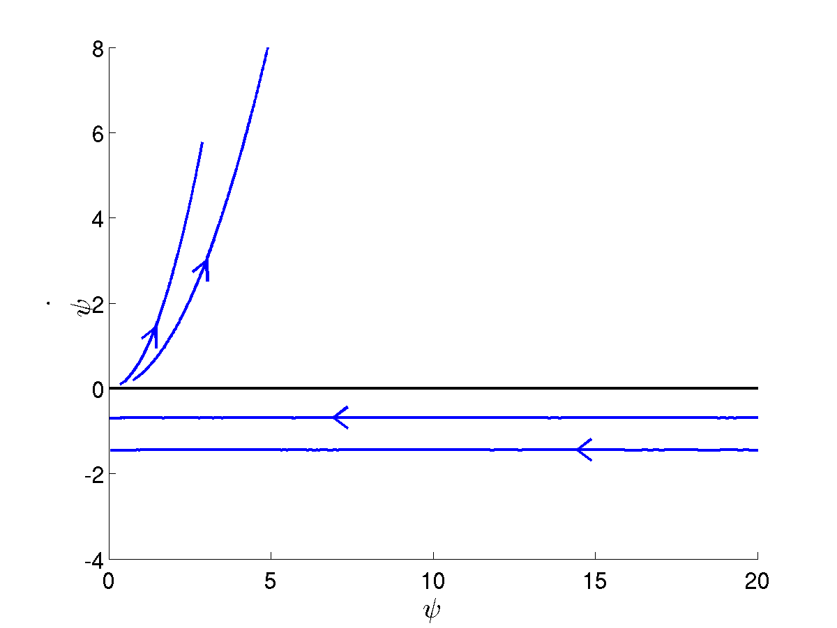 Figure 13
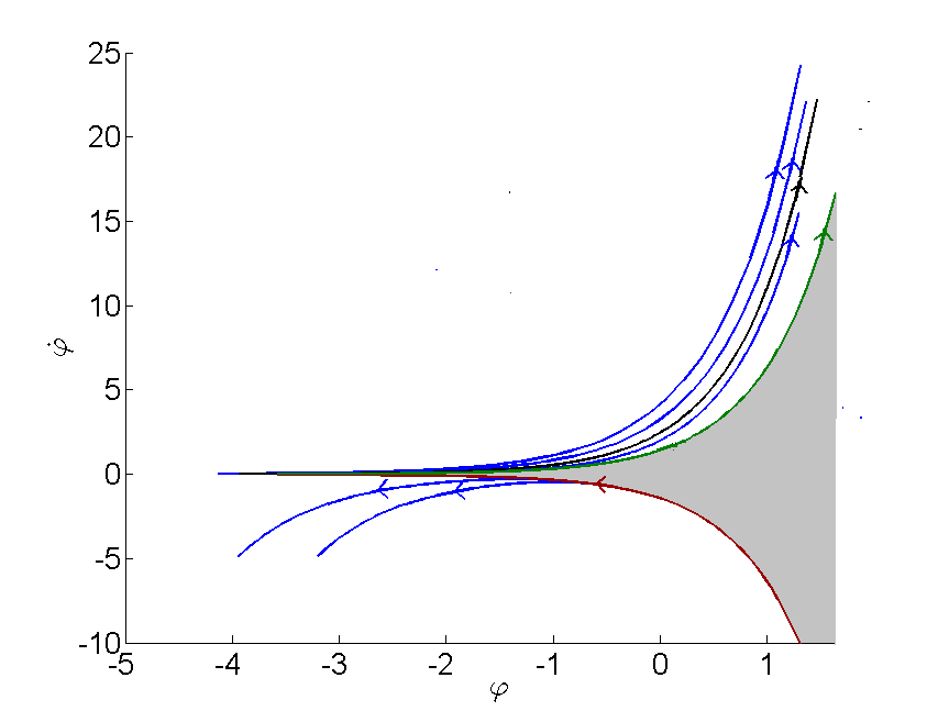 Figure 14
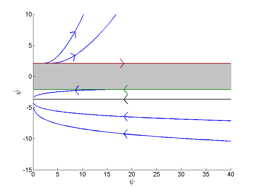 Figure 15
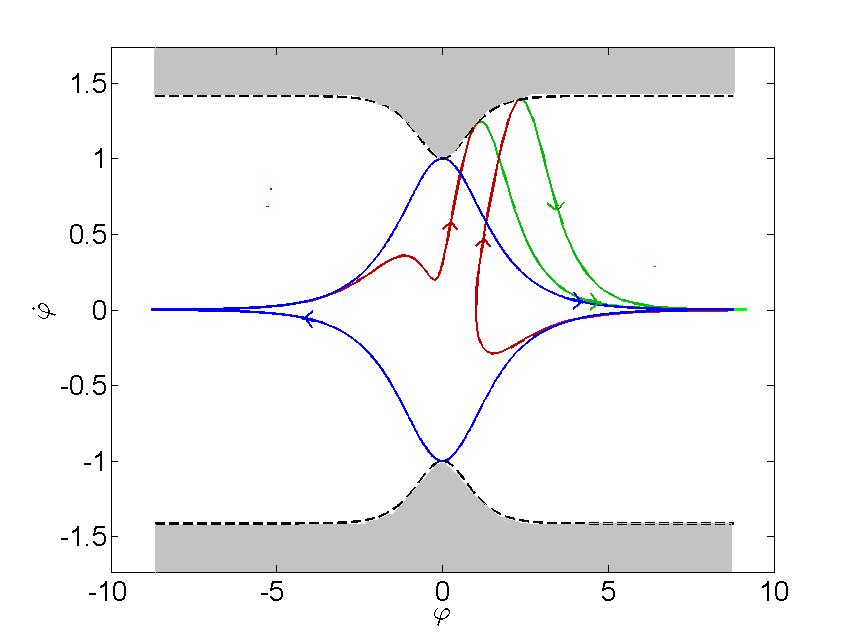 Figure 16
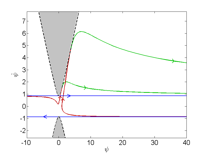 Figure 17
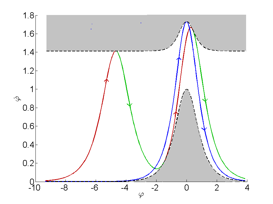 Figure 18
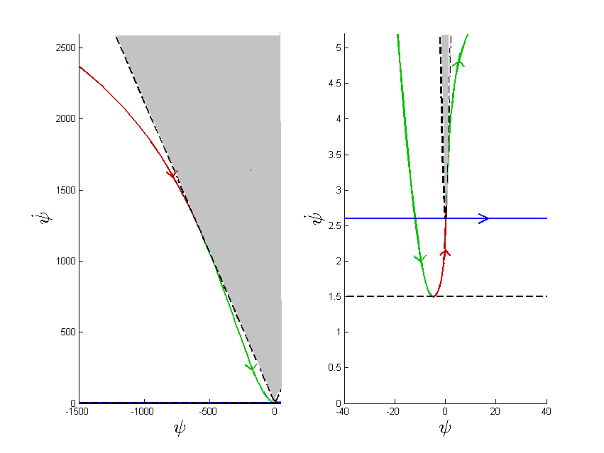 Figure 19
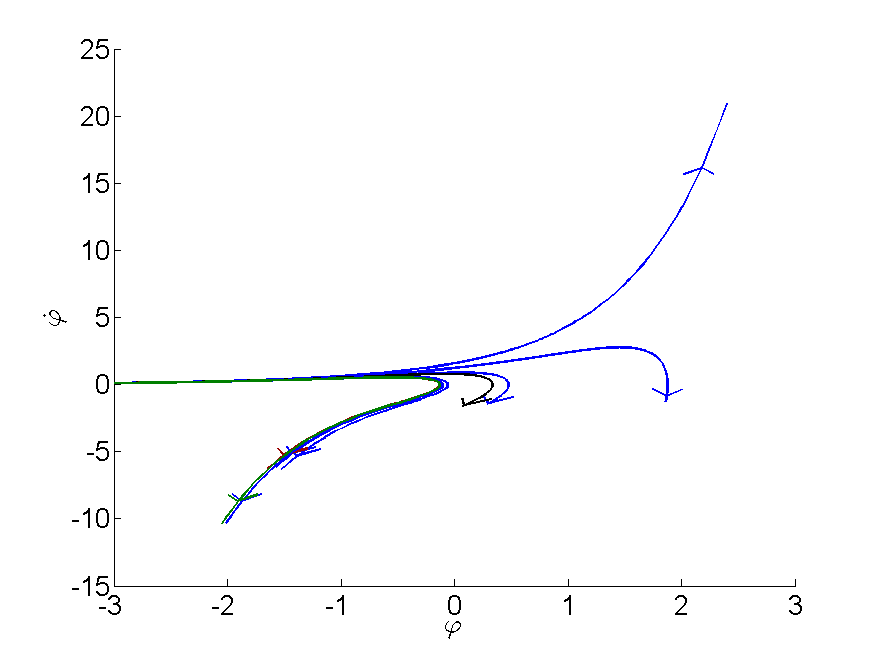 Figure 20
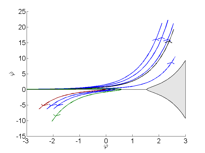 Figure 21
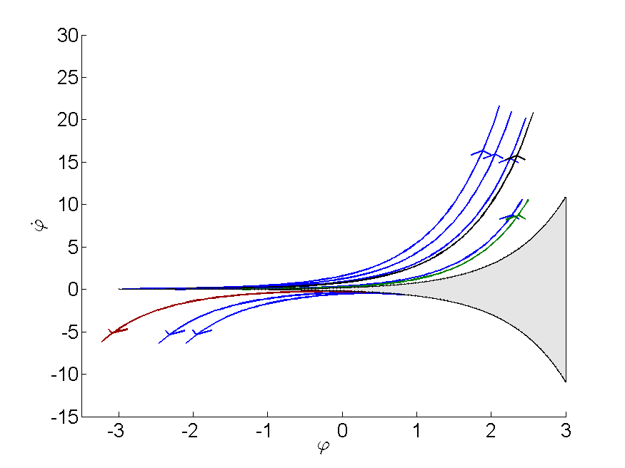 Figure 22
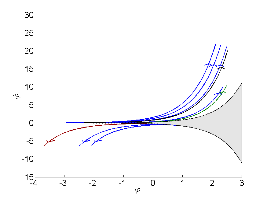 Figure 23
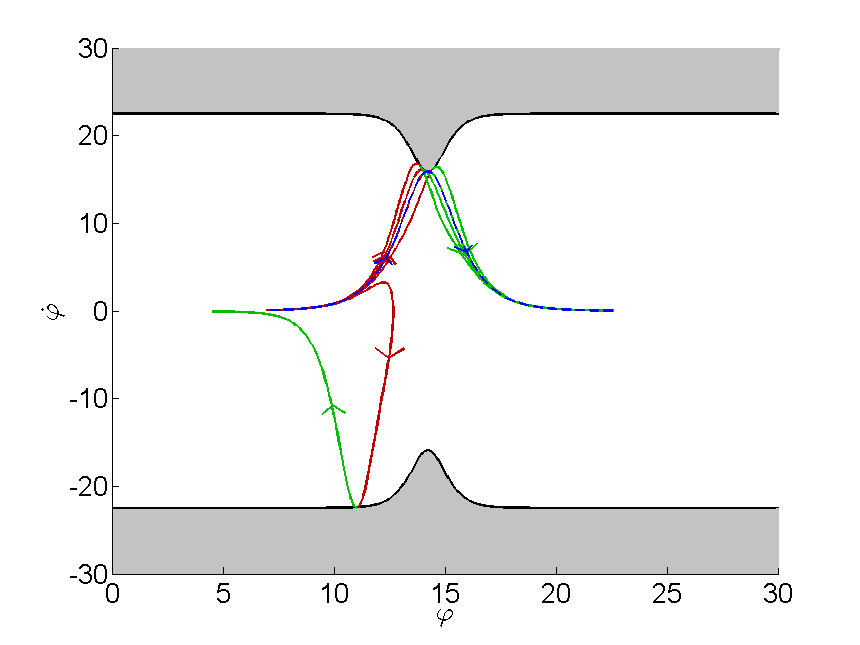 Figure 24
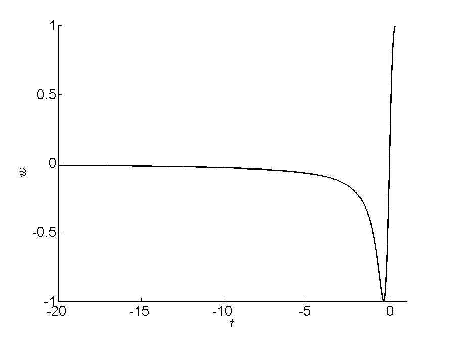 Figure 25
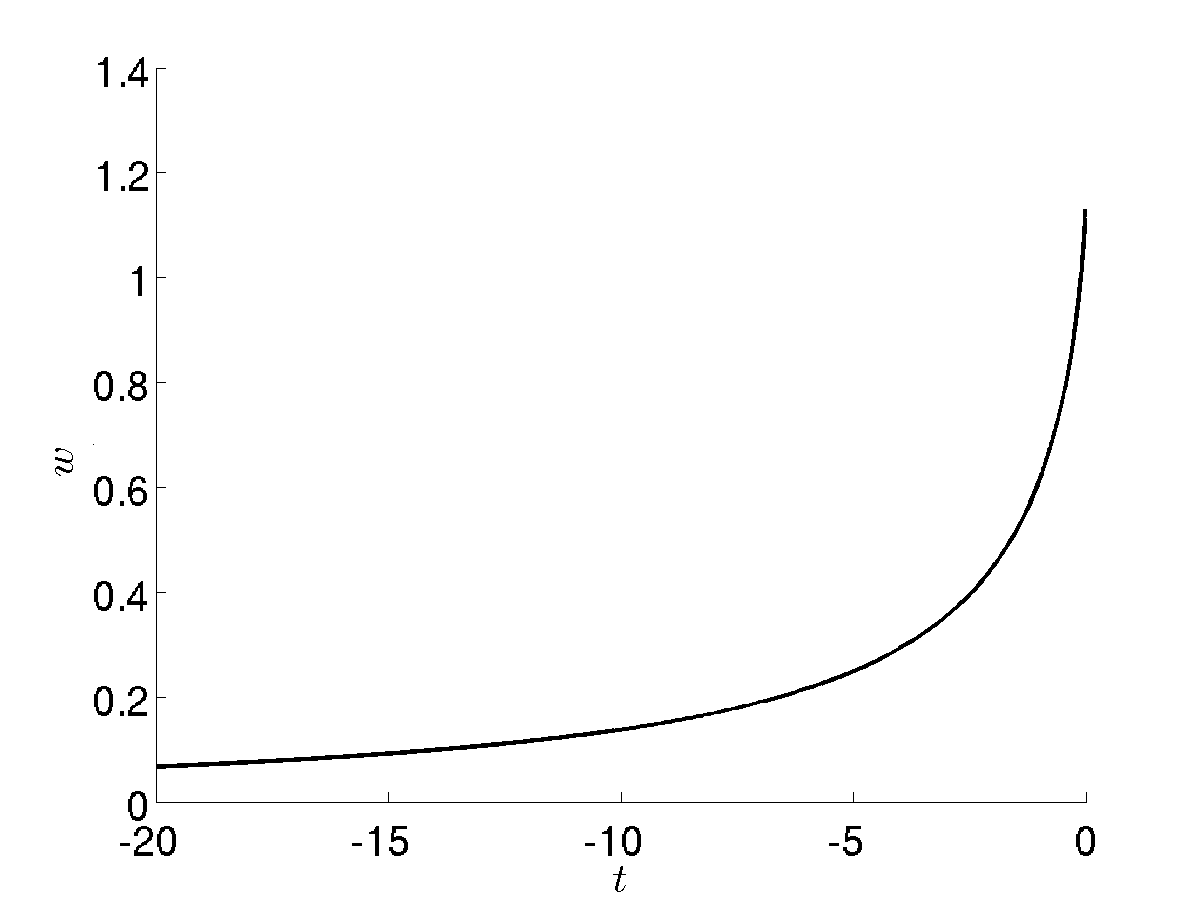 Figure 26
 Figure 27
 Figure 28
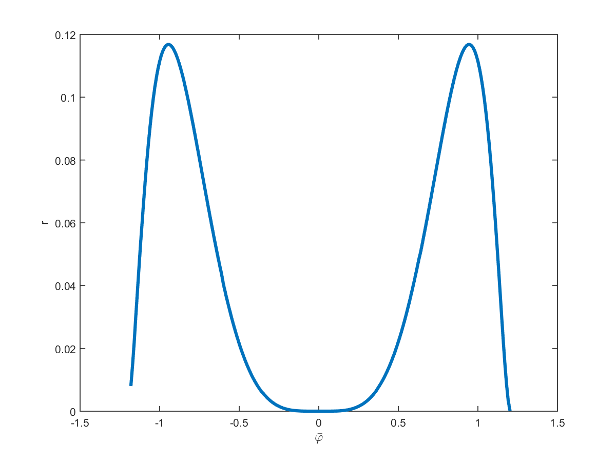 Figure 29
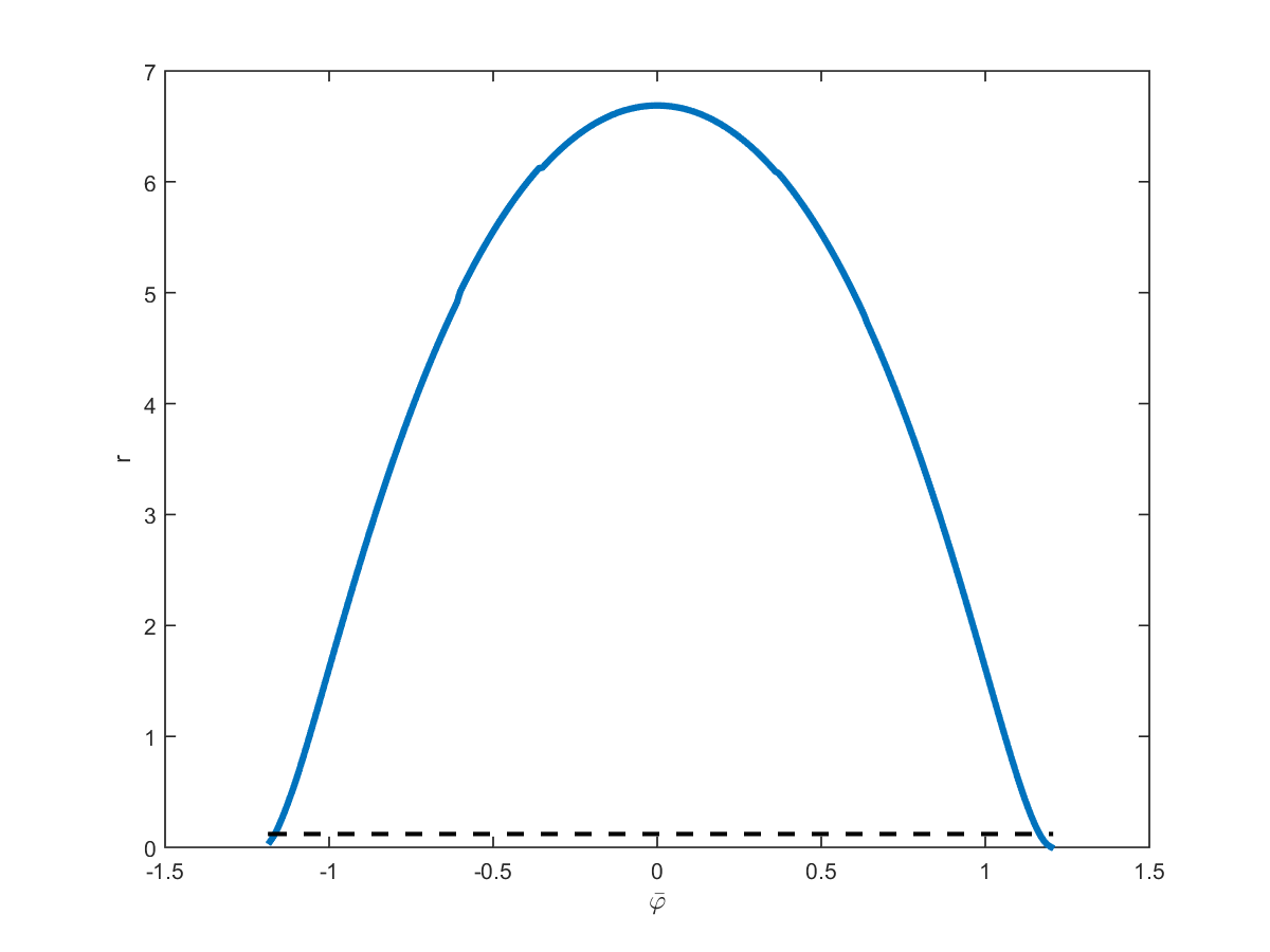 Figure 30
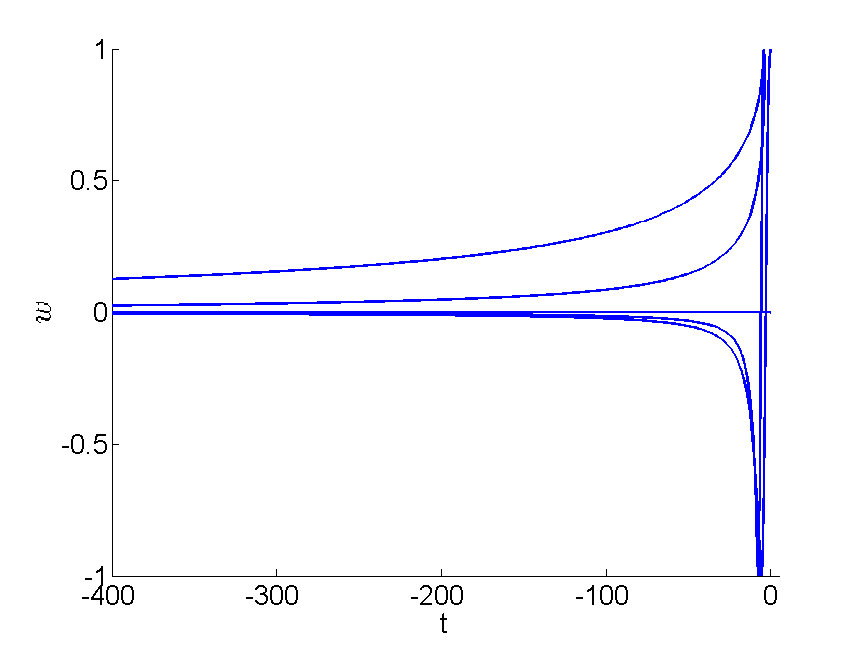 Figure 31
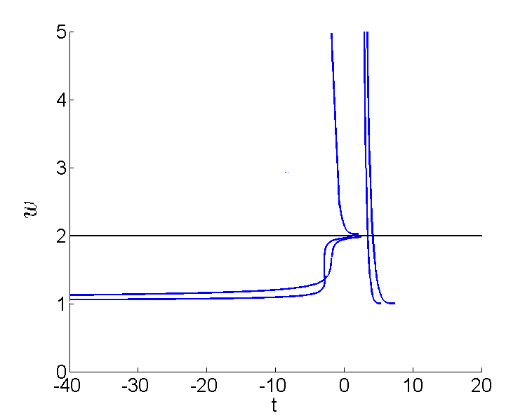 Figure 32
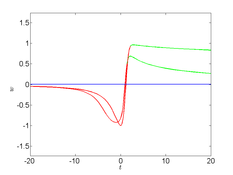 Figure 33
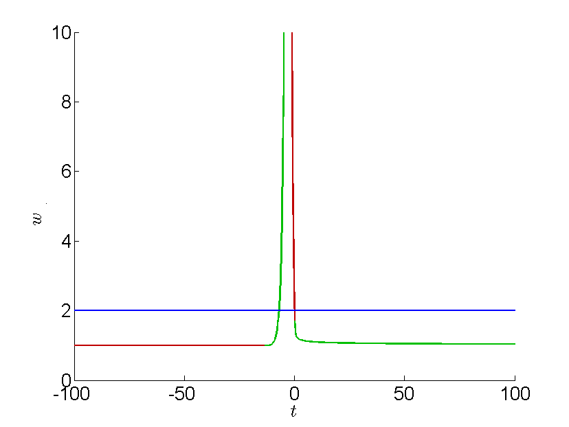 Figure 34
Peer Reviews
No public reviews on file for this paper yet. If you reviewed it on a platform where reviews are public (OpenReview, ICLR, NeurIPS, ICML), you can paste yours below so the community can read it here.
Videos
No videos yet. Explain this paper in a talk, walkthrough, or lecture? Add one.
The matter-ekpyrotic bounce scenario in Loop Quantum Cosmology
Jaume Haroa,111E-mail: [email protected], Jaume Amorósa,222E-mail: [email protected] and Llibert Aresté Salóa, 333E-mail: [email protected]
Abstract
We will perform a detailed study of the matter-ekpyrotic bouncing scenario in Loop Quantum Cosmology using the methods of the dynamical systems theory. We will show that when the background is driven by a single scalar field, at very late times, in the contracting phase, all orbits depict a matter dominated Universe, which evolves to an ekpyrotic phase. After the bounce the Universe enters in the expanding phase, where the orbits leave the ekpyrotic regime going to a kination (also named deflationary) regime. Moreover, this scenario supports the production of heavy massive particles conformally coupled with gravity, which reheats the universe at temperatures compatible with the nucleosynthesis bounds and also the production of massless particles non-conformally coupled with gravity leading to very high reheating temperatures but ensuring the nucleosynthesis success. Dealing with cosmological perturbations, these background dynamics produce a nearly scale invariant power spectrum for the modes that leave the Hubble radius, in the contracting phase, when the Universe is quasi-matter dominated, whose spectral index and corresponding running is compatible with the recent experimental data obtained by PLANCK’s team.
aDepartament de Matemàtica Aplicada, Universitat Politècnica de Catalunya
Diagonal 647, 08028 Barcelona, Spain
Pacs numbers:
1 Introduction
Bouncing cosmologies and more specifically the matter bounce scenario (see [1] for a review of this kind of cosmologies) is the most promising alternative to the inflationary paradigm. There are many ways to obtain cosmologies without the Big Bang singularity: for example violating the null energy condition in General Relativity by incorporating new forms of matter such as phantom [2] or quintom fields [3], Galileons [4] or phantom condensates [5], or by adding terms to Einstein-Hilbert action [6], but the simplest one is to go beyond General Relativity and consider holonomy corrected Loop Quantum Cosmology (LQC), where a Big Bounce replaces the Big Bang singularity [7]. In fact, other future singularities such as Type I (Big Rip) and Type III (Big Freeze) are also forbbiden in holonomy corrected LQC [8].
On the other hand, it is well known that a matter domination period in the contracting phase is dual to the de Sitter regime in the expanding phase [9], which provides a flat power spectrum of cosmological perturbations in the matter bounce scenario. Moreover, an abrupt ekpyrotic phase transition is needed, in the contracting phase, in order to solve the famous Belinsky-Khalatnikov-Lifshitz (BKL) instability: the effective energy density of primordial anisotropy scales as in the contracting phase [10] and, more important, to produce enough particles which will be responsible for thermalizing the universe in the expanding phase [11, 12]. This new scenario named matter-ekpyrotic scenario was introduced in [13], being developed within the two-field model in [14], while in [15] there is a numerical discussion on the primordial anisotropy issue (see [16] for a review). It was treated in the context of Loop Quantum Cosmology in [17], showing that it could be compatible with the new experimental data [18] provided by PLANCK’s team (see also [19]).
The main goal of the present work is to study mathematically, from the viewpoint of the dynamical systems theory, the matter-ekpyrotic scenario in the context of holonomy corrected LQC. More precisely, we study its background dynamics and the evolution of cosmological scalar perturbations in this scenario, showing that it leads to a nearly flat power spectrum of perturbations, whose spectral index and running match correctly with the recent experimental data. Moreover, we will also point out that the phase transition, in the contracting epoch, from matter domination to the ekpyrotic phase, is the responsible for the production of enough particles whose energy density, in the expanding phase, will be dominant, leading to a reheating temperature compatible with the nucleosynthesis bounds.
The work is organized as follows: The dynamical study of the matter-ekpyrotic scenario in General Relativity is performed in section II. In section III we study the dynamics of the background, demonstrating that in Loop Quantum Cosmology the matter-ekpyrotic scenario has two different regimes: at very early times, the universe in the contracting phase is matter dominated and evolves to an ekpyrotic regime, and after the bounce, we show that the universe leaves the ekpyrotic phase and enters in a kination (or deflationary) regime [20]. Section IV is devoted to the calculation of the power spectrum of scalar perturbations in this scenario, showing that the power spectrum is proportional to the square of the value of the Hubble parameter at the transition time. The mechanism to reheat the universe is studied in section V, where we show that the phase transition from the matter to the ekpyrotic regime is essential to produce enough particles to reheat the universe. In last section, we build a simple potential in this scenario that leads to theoretical values of the spectral index and its running that fit well with the last observational data provided by PLANCK’S team.
The units used throughout the paper are and, thus, the reduced Planck’s mass is .
2 Matter-ekpyrotic scenario in General Relativity: The background
In this section, we consider the flat Friedmann-Lemaître-Robertson-Walker (FLRW) metric in the context of General Relativity. Then, the Friedmann, conservation and Raychauduri equations are respectively given by
[TABLE]
where is the Hubble parameter, the energy density and the pressure.
To achieve the matter-ekpyrotic scenario we will deal with a single scalar field, namely . Then, the energy density and pressure are
[TABLE]
being the potential.
Our first goal is to mimic, with a single scalar field , a fluid with Equation of State (EoS) , i.e., we want to obtain a potential which provides a solution of the conservation equation that leads to the same background as a barotropic fluid with EoS , where .
The first step is to write the EoS as follows
[TABLE]
which means that for the potential must be positive, negative for , and vanishes for .
On the other hand, for a fluid with EoS , the Friedmann and conservation equations of General Relativity could be easily solved, giving as a result the background
[TABLE]
Secondly, using the Raychauduri equation one has , and if we only consider increasing functions, i.e., we will obtain
[TABLE]
where (resp. ) refers to the contracting (resp. expanding) phase. In fact, is defined for , and in .
Finally, to reconstruct the potential we use the relation and the Raychaudhuri equation, to obtain
[TABLE]
Using (5), a simple calculation leads to
[TABLE]
and, by writing
[TABLE]
the analytical solution (5) becomes
[TABLE]
We note that this equation is mathematically singular for , which should be treated separately. In this case, since one cannot use the parameter but is only able express the scalar fields through the parameter , as shown in (5). On the other hand, with regards to the trivial case of , it corresponds to a constant , a constant scalar field and a constant potential .
2.1 Dynamical analysis
Once we have obtained the potential for a single scalar field, the dynamical equations (Friedmann and conservation) are
[TABLE]
where .
The conservation equation is a second order differential equation, meaning that there are infinitely many solutions that depict different universes. For example, if one deals in the expanding phase, i.e. we take , then for the potential , the analytical solution with , defines a Universe with EoS all the time. However, the other solutions do not define a Universe with this EoS all the time.
For this reason, what we want to study is the behaviour of the analytical solution (9), i.e., we want to know whether the orbit in the plane defined by the solution (9) will be an attractor or a repeller.
To do that, first of all we study the dynamics in the contracting phase. Performing the change of variable [21]
[TABLE]
the conservation equation will become
[TABLE]
that could be written as a first order one-dimensional differential equation:
[TABLE]
where
[TABLE]
To perform the dynamical study we have to differentiate between cases:
. In this case the differential equation becomes:
[TABLE]
which means that in the half plane , one has and the general solution is given by
[TABLE]
That is, there are two kind of orbits in the plane
[TABLE]
with , and
[TABLE]
The first kind corresponds to a stiff fluid because leads to . And the second kind are fixed points that correspond to .
On the other hand, in the plane , it is easier to study directly the conservation equation
[TABLE]
obtaining
[TABLE]
We point out that orbits and are not stable in the following sense: We consider for example and we make a small perturbation taking , then the modulus of the difference between and , namely , is equal, at the leading order, to . Therefore, one can trivially see that as . Nevertheless, what is important is that all the orbits in the phase space for correspond to a universe which obeys throughout all the evolution of time to the same Equation of state, namely .
. The system has one fixed point, namely
[TABLE]
which is a global repeller because , and for , is negative, which means that in cosmic time the orbits move away from .
This solution corresponds to
[TABLE]
whose orbit depicts, all the time, in the contracting phase, a Universe with EoS .
Note that the fact that solution (22) is a repeller means that all orbits depict, at early times, a universe with equation of state , which will be a matter dominated Universe in the particular case when . Moreover, since time goes forward, the solutions separate from (22), meaning that the backgrounds depicted by them cease to satisfy this equation of state. The phase portrait is drawn in Figure 2.
In this scenario, a fundamental quantity is the effective EoS parameter, namely
[TABLE]
which could be used to indicate the evolution of the EoS for each orbit of the dynamical system. In Figure 3, we can see that all orbits tend asymptotically at the beginning of the contracting phase to .
. The system is only defined for . Moreover, the system has three fixed points, namely
[TABLE]
is an attractor in the half plane because and are repellers because these solutions correspond to , and in the contracting phase decreases as time goes forward, that is, the orbits moves away from .
The first solution corresponds to
[TABLE]
whose orbit depicts, all the time, in the contracting phase, a Universe with EoS . The other ones satisfy .
Since the orbit is an attractor in the half plane , this means that all the other orbits in the half plane depict, at late time, a Universe with EoS .
Note that in Figure 4, orbits approaching either of the fixed points reach such value (corresponding to ) in a finite cosmic time. Since near the dynamical system behaves as , it is reached in a finite time. Given that is finite, is finite as well and, hence, in a finite cosmic backward time the contracting phase starts after . This means that these orbits can be extended backward in time to the expanding phase. Hence, going forward in time one can argue that these orbits depict a bouncing universe, but this is not a good bounce, because the universe moves from the expanding to the contracting phase and, moreover, the bounce occurs at . As we will see in next Section dealing with Loop Quantum Cosmology, the bounces we are interested in are those that come from the contracting to expanding phase and such that at the bouncing time the energy density is very high.
On the other hand, the orbits such that start from an initial value corresponding to , which takes places at and evolve towards .
In Figure 5 we show the evolution of . We see that for those orbits approaching to the analytical solution in the plane , at late times tends to , while for those in which diverge, tends to . Regarding early times, those orbits coming from an infinite value of are those that have started the contracting phase for a finite value of time in the values , while the orbits that have started the contracting phase for approach backwards in time to the value .
Remark 2.1**.**
The same analysis shows that, in the expanding phase, for there are solutions that correspond to a stiff fluid, and others with . For the solution that depicts a fluid with EoS is an attractor. For , the solution that depicts a fluid with EoS is a repeller, and the one with an attractor.
Once we have performed this previous study, it is interesting to consider the matter-ekpyrotic scenario given, in the contracting (resp. expanding) phase, by a potential () with the shape
[TABLE]
with and .
In Figure 6 we show phase portraits, in contracting phase, for the superposed potential (26) with and . The colouring code is that the black, red, green solutions are those given by the initial condition of the corresponding critical orbits in the case . Moreover, in Figure 7 we have drawn the parameter for black orbits in each superposition with .
From our previous study it seems clear that in the contracting phase, at early times, all the orbits will depict a matter dominated Universe, and after leaving this behaviour they will evolve, at late times, to an ekpyrotic one. On the contrary, in the expanding phase, at early times, orbits will depict a Universe in the ekpyrotic phase that eventually evolves to a matter dominated one.
3 The matter-ekpyrotic scenario in Loop Quantum Cosmology: The background
Basically, Loop Quantum Cosmology (LQC), where holonomy corrections are introduced due to the assumption of the discrete nature of the space-time, could be built following three steps:
In GR, for the flat FLRW geometry, one takes a cell of volume , the gravitational part of the Hamiltonian is , and the usual canonical conjugate variables are the pair . In LQC these canonically conjugate variables are replaced by the Ashtekar connection and its conjugate momentum (the densitized triad), that we will denote respectively by and , and which are related with the standard variables via the relation [22]
[TABLE]
where is the Barbero-Immirzi parameter, whose numerical value is obtained comparing the Bekenstein-Hawking formula with the black hole entropy calculated in Loop Quantum Gravity (LQG) [23]. The Poisson bracket for these variables satisfies . Moreover, in LQC another pair of canonically conjugate variables , named new variables, satisfying and defined as and , are usually used. 2. 2.
The quantization of GR via the Wheeler-DeWitt equation in the -representation is based on the Hilbert space , which shows the continuous nature of the space (the scale factor has a continuous spectrum). However, in LQC the Hilbert space is the space of almost periodic functions, i.e., functions of the form [24]
[TABLE]
with and being a square-summable sequence (), provided by the inner product (in the -representation)
[TABLE]
The orthonormal basis of this space are functions of the form , and the quantum operator corresponding to the momentum , in this representation, is given by . Thus, the ortonormal states are eigenvectors of , which proves that its spectrum is discrete, showing the discrete nature of the space in LQC [25]. However, the variable (and also ) does not have a well-defined quantum operator , because the norm of diverges. For this reason it is important to introduce holonomies [26] obtained by integrating the Ashtekar connection along a curve , where depends on the length of the curve and which has a well-defined quantum operator in the Hilbert space. 3. 3.
In these variables the gravitational part of the Hamiltonian becomes
[TABLE]
which contains the variable or , and thus it does not have a well-defined quantum analogue. Then, and this is a key point in LQC, one has to “regulate” (in fact, this means approximate) the Hamiltonian, obtaining another one that contains quantities that could be quantized. Working in the -representation this could be done using the holonomies , where now is a parameter with the dimensions of length, whose numerical value is obtained, invoking the quantum nature of the space, identifying its square with the minimum eigenvalue of the area operator in Loop Quantum Gravity, namely [27]. This regularized gravitational part of the Hamiltonian has a complicated expression in terms of the holonomies [26, 25, 24], but after some algebra it reduces to [28, 29]
[TABLE]
where denotes the total Hamiltonian of the system. Note also that, when goes to zero, it becomes the usual Hamiltonian in GR.
Finally, the Hamilton equation is equivalent to the equation
[TABLE]
that together with the Hamiltonian constraint, i.e., , leads to the Friedmann equation in LQC [7]
[TABLE]
where is the so-called critical energy density.
It is important to realize that this equation depicts an ellipse in the plane , which is a bounded curve, meaning that the Big Bang singularity is removed in this theory. In fact, it is replaced by a Big Bounce when the universe reaches the critical energy density . Moreover note that the energy density lies between [math] and and the Hubble parameter between and . This is a great difference in contrast with GR, where the Friedmann equation depicts a parabola in the plane allowing the Big Bang singularity because this curve is unbounded.
Once again, we want to mimic by a scalar field a fluid with EoS . Solving the Friedmann and conservation equations in LQC for this kind of fluid one has the solution [30]
[TABLE]
Then, the equation becomes
[TABLE]
whose solution is given by [31]
[TABLE]
To reconstruct the potential we use the formula
[TABLE]
and we isolate as a function of , obtaining [30]
[TABLE]
where we have chosen .
We can see, as in the case of General Relativity, for the potential vanishes, it is positive for and negative for . As in General Relativity, we will differentiate between cases so as to study the following dynamical system:
[TABLE]
where .
. In this case the differential equation becomes:
[TABLE]
obtaining for orbits in the plane of the form
[TABLE]
where , and for
[TABLE]
where . And finally the trivial solution from the previous equation would correspond to , corresponding to .
Now, we proceed to the stability analysis analogous to the one performed in the case of GR. If we consider for instant in a small perturbation , then one obtains that
[TABLE]
Moreover, we observe that tends to 0 both at (i.e the bounce, the end of contracting phase) and at (end of expanding phase). Therefore, all orbits are stable and, furthermore, all orbits foliating the phase space satisfy throughout all the evolution of time the equation of state .
In order to study the remaining two cases, it is suitable to perform the following change of variables, motivated by (36):
[TABLE]
Hence, equation of conservation becomes
[TABLE]
where and . 2. 2.
. The dynamical system is defined for and has two fixed points:
[TABLE]
In Figure 8, we have represented the phase portrait of the dynamical system, such that blue orbits stand for the analytical ones (fixed points , corresponding to equation (36)), red colour is for the contracting phase and green colour is for the expanding phase. The coloured zone in the phase portrait is the forbidden region, in which . Note that the bounce from the contracting to the expanding phase happens in curve. We see that there are two types of orbits: those that cross axis and those that cross axis . Therefore, it can be clearly concluded that the analytical orbit is a repeller in the contracting phase and an attractor in the contracting phase, as one can also verify with the effective EoS parameter in Figure 9.
. The dynamical system is defined for and has four fixed points:
[TABLE]
As already happened with General Relativity for the case, those orbits approaching (corresponding to ) reach it at a finite time because of the same argument that was used in General Relativity, since holonomic corrections can be discarded near . Therefore, in these cases we will see a bounce at . In the phase portrait in Figure 10 (with the same colour notation as in the former case), we have seen that all orbits different from the analytical one (, corresponding to (36)) perform two cycles in the ellipse, with two bounces at and one bounce at . The process is the following:
- •
Contracting phase 1: At , for infinite values of and and at a finite time the orbit reaches , occurring a bounce.
- •
Expanding phase 1: After the first bounce, the orbit enters into the expanding phase reaching either or (corresponding to ) at a finite time . There, another bounce occurs.
- •
Contracting phase 2: After the second bounce, the orbit starts the second cycle in the ellipse and reaches at a finite time (third bounce).
- •
Expanding phase 3: After this last bounce, the orbit enters into the expanding phase and tends asymptotically for to for infinite values of both and .
Therefore, we infere that the analytical solutions are attractors in the contracting phase and repellers in the expanding phase, while the solutions are repellers in the contracting phase and attractors in the expanding phase. With regards to the behaviour of , represented in 11, it is seen that both at and , , whereas it diverges at the bounce at .
From these previous results, to obtain a simple version of the matter-ekpyrotic bouncing scenario in LQC, we can consider the potential
[TABLE]
where , and and the abrupt phase transition, needed in order to produce enough particles to reheat the universe, occurs at .
For this potential some orbits will lead to an effective EoS being zero at early times, approximately just before the bounce, and finally approaching asymptotically to in the expanding phase. These orbits could be obtained by taking as an initial condition a point corresponding to an orbit in the second cycle of the figure 10. Thus, with these initial conditions, integrating the conservation equation, one will set up, for the potential (50), orbits with an effective EoS parameter satisfying the required properties.
In fact, in last section we will obtain a potential which leads to a viable matter-ekpyrotic bounce scenario, i.e., a scenario which provides theoretical values of the spectral parameters that match at Confidence Level with the recent observational data.
Some final remarks are in order:
As we have already explained in the introduction, holonomy corrections provide a Big Bounce. Then, the conservation equation
[TABLE]
has to be studied in the contracting and expanding phase. Firstly, the contracting phase, i.e. with , takes place and, when the Universe bounces at , it enters into the expanding one and, thus, its dynamics will now be given by the conservation equation with . 2. 2.
Note also that, in Loop Quantum Cosmology, when one considers one has to use the last formula of (23), i.e., , because the intermediate one only holds in General Relativity (when holonomy corrections can be disregarded). 3. 3.
In [17], the authors obtain an ekpyrotic phase with the following potential:
[TABLE]
When , this potential is symmetric and, by using the change of variables , the new potential becomes which has the asymptotic behaviour as our former potential for .
If , the bounce at () takes place at . Therefore, in this case, all orbits have two cycles except the one bouncing at , which has a single cycle, as we can see in Figure 12. However, this last orbit does not correspond to the analytical solution since the value of does not remain constant, but approaches asymptotically to 1 for both and , as we can see in Figure 13.
Nevertheless, when a sufficiently low is used, orbits do not reach in a finite time and, hence, they have a single cycle, as we can see in Figures 14 and 15.
4 The power spectrum in the matter-ekpyrotic bounce scenario
In this section we will calculate explicitly the power spectrum of cosmological perturbations in the matter-ekpyrotic bounce scenario. In Loop Quantum Cosmology the corresponding Mukhanov-Sasaki equation [32], in Fourier space, is given by [33]
[TABLE]
where the velocity of sound is given by , , being ′ the derivative with respect the conformal time and the conformal Hubble parameter.
During the matter-domination period, when , i.e., far enough from the bounce in the contracting phase, the holonomy corrections could safely be disregarded and the equation (53) becomes the usual Mukhanov-Sasaki equation in GR
[TABLE]
On the other hand, it is well-known that, in conformal time, when the universe is matter dominated and the holonomy corrections can be disregarded, the scale factor evolves as follows [17]
[TABLE]
with , and is the transition time, where it is assumed that the phase transition occurs far from the bounce and, once again, the GR is a good approximation.
Therefore, since at early times during the matter-domination, in the contracting phase, the energy density is smaller than the critical one, one can use the equation (54) instead of (53), whose Bunch-Davies vacuum will be given by the well-known modes [17]
[TABLE]
The modes will eventually leave the Hubble radius, and thus, when they are well outside of the Hubble radius, i.e., when they satisfy ,
[TABLE]
On the other hand, for these modes, up to their reentry in the Hubble radius in the expanding phase, we can use the long-wavelenght approximation, and the Mukhanov-Sasaki equation (53) becomes
[TABLE]
whose solution is given by
[TABLE]
which is valid from the exit in the contracting phase to the reentry into the Hubble radius in the expanding one, and thus, also during the bounce.
To obtain the coefficients and , we note that in a matter dominated universe at early times, is given by , because the holonomy corrections could be disregarded. A simple calculation leads to
[TABLE]
Matching both expressions, we obtain the following values of and
[TABLE]
and thus, the curvature fluctuation in co-moving coordinates is given by
[TABLE]
Note that, if is continuous, at the transition time , the formula (4) holds for every time, and we can calculate the power spectrum as
[TABLE]
where, when the asymptotic form of is given by (55), i.e., at very early times . This is essential in order to perform numerical calculations, because once an orbit has been chosen, the value of is given by formula (33), the value of is obtained from the relation , the asymptotic condition at early times and the value of via the relation .
Remark 4.1**.**
It is important to realize that formula (4) is only valid for the modes that leave the Hubble radius in the matter dominated epoch, i.e., when the holonomy corrections could be disregarded and the square of the velocity of sound is equal to . However, in the so-called super-inflationary phase (), the velocity of sound becomes imaginary, which could lead, during this stage, to a Jeans instability for ultra-violet modes satisfying .
Consequently, these sub-horizon growing modes could condensate, and after leaving the Hubble radius, they could produce undesirable cosmological consequences. Sometimes, in LQC, it is argued that its wavelength is too small to be detected or directly this problem is not discussed, but really what happens is that, during this regime, the validity of the linear perturbations equations does not seem likely. This is one of the reasons why a Teleparallel version of LQC has been introduced in [34]. This theory is based on the following two points: 1.- For the FLRW geometry, the holonomy corrected Friedmann equation (33) could be obtained as a particular case of a teleparallel theory. 2.- The perturbation equations of lead to a modified Mukhanov-Sasaki equation with a square of the velocity of sound always positive, and thus, avoiding the Jeans instability.
As an example, if one disregards the phase transition, i.e., if one only considers a matter domination during all the background evolution, and one uses the orbit given by the solution (36) with , formula (4) leads to the result (see [30] and [34] for a derivation of the result), where is the Planck’s energy density, which is incompatible with the experimental data [35], because in LQC the value of the critical density is given by . This means that, to be viable, the matter bounce scenario must be implemented, for example, with an ekpyrotic phase transition.
In this way we can introduce a transition. However, when it is too abrupt, formula (4) does not hold. To be more precise, we consider the simple example [17] where the scale factor is given, in terms of the cosmic time, by
[TABLE]
where , being the value of the Hubble parameter at the time of the phase transition and is the time when the universe enters in a deflationary or kination regime. So that the Hubble parameter be continuous at one has to choose
[TABLE]
where we have used that .
In [17] the authors heuristically obtained that . Then, since the observational values of the power spectrum states , one will deduce that .
To reproduce mathematically this result we consider, for , the solution in the long wave-lenght approximation
[TABLE]
then matching at one obtains
[TABLE]
That is,
[TABLE]
because for modes well outside to the Hubble radius one has .
First we are interested in the evolution of during the ekpyrotic regime.
For this reason we will calculate
[TABLE]
where we have used that, during the ekpyrotic phase,
[TABLE]
Performing the change of variable one obtains
[TABLE]
The integrals that appear in this expression are of the same order as
[TABLE]
[TABLE]
because in this model .
Finally, using that , we will get
[TABLE]
and, approximately, we have
[TABLE]
During the deflationary phase, the curvature fluctuation evolves as
[TABLE]
Thus, performing the matching at one obtains
[TABLE]
The deflationary regime ends when the universe becomes reheated and enters in a radiation dominated phase. For this reason we have to calculate
[TABLE]
Using the formulas and of [36]
[TABLE]
and the fact that and , one obtains
[TABLE]
where is the reheating temperature. Now, taking into account that in LQC and that the nucleosynthesis bounds impose , one has
[TABLE]
If we impose the first term on the right hand side to be greater than the second one, one will have the constraint
[TABLE]
Now, with this assumption one will have
When the universe enters in a radiation dominated phase one will have
[TABLE]
where the holonomy corrections could be disregarded and then, with . Matching at one will get
[TABLE]
A simple integration shows that, at very late times
[TABLE]
This last quantity is equal to
[TABLE]
where we have used that during the deflationary phase one has
[TABLE]
Then, we conclude that, if satisfies the conditions , one will have , which means that the power spectrum is given by
[TABLE]
and thus, to match with observational data one has to choose . Finally, the condition is fulfilled for .
Remark 4.2**.**
As we have already explained, when one deals with a matter dominated Universe (without the ekpyrotic phase transition), the power spectrum of cosmological perturbations is of the order , and since LQC provides a value around Planck’s density, its value is in contradiction with the current observations because it is too high. This is another reason to implement an ekpyrotic phase in the matter bounce scenario.
5 The reheating process
We will consider a heavy massive quantum field, namely , conformally coupled with gravity, and first of all we consider the model (67) proposed by [17]. This model has been studied in [12], where it has been shown that the energy density of the produced particles is given by
[TABLE]
During the ekpyrotic phase, the background evolves as , then, since , during the contracting phase increases faster than , and thus, the Universe continues being driven by the background. However, after the bounce, the Universe enters in a kination () regime and the background evolves as , where
[TABLE]
is the minimum value of the scale factor. Since in the expanding phase decreases as and as , the energy density of the created particles will eventually start to dominate, and at that moment, namely , when both energy densities will be of the same order, the Universe will become reheated with a temperature .
To calculate this temperature we use the identity to obtain
[TABLE]
where . And, thus, the reheating temperature is given by
[TABLE]
Taking into account, as we have shown in Section , that for one has , one will obtain in Figure 16 the dependence of as a function of .
Consequently, since nucleosynthesis bounds constrain the reheating temperature to be between and , from Figure 16 we can see that the matter-ekpyrotic model only holds when is of the order . However, the reheating temperature is very high and is in the borderline. Then, if one wants a lower reheating temperature, one has to consider a phase transition less abrupt than the one considered above. To do this, we will consider the model defined in next section, where in the phase transition the second derivative of the Hubble parameter is discontinuous.
Assuming that the mass of the quantum field is very high, for example is of the order of the reduced Planck mass, we could approximate the vacuum modes by its first order WKB solution, obtaining that the Bogoliubov coefficient is given by [12, 37]
[TABLE]
The energy density of the produced particles is given by
[TABLE]
On the other hand, after the phase transition the energy density of the background evolves as , and after the bounce, since the universe enters in a kination domination, it evolves as , where the value of the scale factor at the bouncing time is given by formula (91).
In the contracting phase, the energy density is always dominant, but in the expanding one it will eventually become subdominant. When both energy densities are of the same order the universe becomes reheated, this happens when
[TABLE]
where the constant has been introduced in (91). Then, the reheating temperature will be
[TABLE]
where . And, after reheating, the universe is dominated by a thermalized relativistic plasma and matches with the standard hot Friedmann universe.
Finally, from formula (97), if one takes, for instance, , one will obtain the picture drawn in Figure 17, which shows that the reheating temperatures belong to the range between and for values of up to order .
Two final remarks are in order:
When one considers very light particles non-conformally coupled with gravity, the energy density of the produced particles is [38, 39], leading to the reheating temperature
[TABLE]
which, as we can see in Figure 18, is always greater that , i.e., the matter-ekpyrotic bounce scenario only supports the creation of massless particles when the reheating temperature of the universe is very high.
The difference between the matter-ekpyrotic scenario and the current models in quintessence inflation is that in the later one the phase transition occurs after the end of inflation and, thus, the value of the Hubble parameter is of the order of [39, 37], leading to a reheating temperature of the order of , which is less than the one obtained in matter-ekpyrotic LQC scenario.
6 Comparison with experimental data
In the matter-ekpyrotic bounce scenario, for modes that leave the Hubble radius at very early times, when the universe is matter dominated, the spectral index and its running are given by [40, 19]
[TABLE]
It is clear that a pure matter-ekpyrotic bouncing scenario leads to
[TABLE]
Then, to match with the current observational data, one needs to improve this scenario introducing a quasi-matter domination period at very early times. To do this, first of all one has to consider the Raychaudhuri equation in LQC (see for instance [41])
[TABLE]
which for the linear EoS becomes
[TABLE]
Then, in the ekpyrotic phase one has to simply choose , and for quasi-matter domination one could choose (we have written for convenience, but in principle can be positive or negative). However, at the phase transition, the derivative of the Hubble parameter is discontinuous and, as we have seen in the previous section, this kind of models could be ruled out by the nucleosynthesis bounds due to its high reheating temperature. For this reason we need to match these dynamics in a continuous way, and a simple way to do this is presented in the following model
[TABLE]
Note that in the contracting phase, near , since holonomy corrections could be disregarded, these dynamics could be written as follows
[TABLE]
Moreover, the effective Equation of State (EoS) parameter, namely , is given by
[TABLE]
Then, we can see that when one has , that is, the universe is quasi-matter dominated.
On the other hand, the potential that leads to these dynamics could be obtained approximately using the reconstruction method, as follows: When holonomy corrections could be disregarded, Raychaudhuri equation becomes , and then, , obtaining for our model, when
[TABLE]
where we have used formula of [36]
[TABLE]
Conversely,
[TABLE]
Since, when holonomy corrections are disregarded, the potential is given by , one has approximately for
[TABLE]
On the contrary, as we have seen in section , in the ekpyrotic phase the potential is given by [30]
[TABLE]
and, since for the potential (114) one has , assuming the continuity of the potential at the transition phase one gets
[TABLE]
Therefore, if one takes into account the approximation
[TABLE]
one will have
[TABLE]
Summing up, the potential we propose in the matter-ekpyrotic bounce scenario is
[TABLE]
Note that when the potential satisfies , that is, the universe is matter dominated at early times, and for the universe is in the ekpyrotic regime.
To perform the calculations, we choose, for example, as a pivot scale where subindex [math] means the current time, and we choose, as usual, [18]. To calculate the value of we need the current value of the scale factor which could be calculated as follows:
For the sake of simplicity we take . Then, from equation (96), the value of the scale factor at the beginning of the radiation era will satisfy .
Now, we use the relation [42]
[TABLE]
to obtain , where we have used that the current temperature of the universe is , and that for the reheating temperature is . Consequently, and, thus since , one concludes that .
On the other hand, let be the time when the pivot scale leaves the Hubble radius during the quasi-matter domination in the contracting phase. Then one will have , which means because the pivot scale leaves the Hubble radius, in the contracting phase, before the phase transition. Then, we can conclude that , and thus
[TABLE]
and
[TABLE]
Planck13 observational data at C.L. give the following results: and . Then, to match our theoretical model, with the -marginalized domain for the spectral index at C.L., one has to choose the effective EoS parameter satisfying
[TABLE]
On the other hand, since we can see that the theoretical value of the running enters in the - marginalized domain for the running at C.L.
A final important remark is in order: As pointed out in [17], in the matter-ekpyrotic scenario, dealing with the analytical solution, the power spectrum of tensor and scalar perturbations are of the same order. This means that the ratio of tensor to scalar perturbations, namely , does not satisfy the constraint provided by the joint analysis data from BICEP2/Keck Array and Planck [46]. There are several ways to address this problem, one of them is to consider at CDM universe at early times [43, 44] because, due to the small velocity of sound, this increases the power spectrum of scalar perturbations and conserves the power spectrum of tensor ones, that is, it suppresses the tensor/scalar ratio. However, one has to realize that these calculations are performed for analytical solutions, but when one deals with a scalar field there are infinitely many solutions. A quantitative study of the match of solutions to in a broad array of solutions has been done in a LQC matter-dominated scenario, both teleparallel and holonomy corrected versions, with , in section 4.1 of [45]. Its results are summarized in Figure 19. The bound is satisfied in holonomy corrected LQC for all possible bounce values of the field , while in teleparallel corrected LQC the bound is satisfied only at the tail cases or . In all cases can go down to 0 in value. Whether the ekpyrotic regime in the early phase affects this match of the theory with the expected value of is a difficult point that deserves future investigation.
7 Conclusions
In the present work we have shown, with all the mathematical details, that the matter-ekpyrotic bounce scenario in Loop Quantum Cosmology, whose background has a matter domination regime in the contracting phase at very early times followed by a phase transition to an ekpyrotic epoch up to the bounce where the universe enters in a kination phase, is a promising alternative to the inflationary paradigm, because it leads to theoretical values of some spectral parameters - the power spectrum of scalar perturbations, the spectral index and its running- that match at Confidence Level with the current observational data. Moreover, the phase transition, produced in the contracting phase, is able to produce enough particles -very massive conformally coupled with gravity or massless non conformally coupled- to reheat the universe, in the expanding phase, at temperatures compatible with the bounds coming from nucleosynthesis, and thus, matching with the hot Friedmann universe.
On the other hand, the drawbacks affecting this proposed LQC matter-ekpyrotic bounce scenario include the uncertainty about the reliability of the linear equations of perturbations for high in the sub-horizon regime due to the Jeans instability of these modes, and the match of the predicted values of the tensor/ scalar perturbation ratio to its observed bounds, which is still an open question.
Acknowledgments. This investigation has been supported in part by MINECO (Spain), project MTM2014-52402-C3-1-P and MTM2015-69135-P.
The reference list from the paper itself. Each links out to its DOI / PubMed record.
- 1[1] M. Novello and S.E. Perez Bergliaffa, Phys. Rept. 463 , 127 (2008) [ar Xiv:0802.1634]. R.H. Brandenberger, (2012) [ar Xiv:1206.4196]. R.H. Brandenberger, Int. J. Mod. Phys. Conf. Ser 01 , 67 (2008) [ar Xiv:0902.4731]. R.H. Brandenberger, AIP Conf. Proc. 1268 , 3 (2010) [ar Xiv:1003.1745]. R.H. Brandenberger, Po S (ICFI 2010) 001 , (2010) [ar Xiv:1103.2271].
- 2[2] L.E. Allen and D. Wands, Phys. Rev. D 70 (2004) 063515 [ar Xiv:0404441].
- 3[3] Y.-F. Cai, T. Qiu, Y.-S. Piao, M. Li and X. Zhang, JHEP 10 (2007) 071 [ar Xiv:0704.1090].
- 4[4] T. Qiu, J. Evslin, Y.-F. Cai, M. Li and X. Zhang, JCAP 10 (2011) 036 [ar Xiv:1108.0593].
- 5[5] C. Lin, R.H. Brandenberger and L. Perreault Levasseur, JCAP 04 (2011) 019 [ar Xiv:1007.2654].
- 6[6] M. Roshan and F. Shojai, Phys. Rev. D 94 , 044002 (2006) [ar Xiv:1607.06049].
- 7[7] A. Ashtekar, T. Pawlowski and P. Singh, Phys. Rev. Lett. 96 141301, (2006) [ar Xiv:0602086]. A. Ashtekar, T. Pawlowski and P. Singh, Phys. Rev. D 74 , 084003 (2006) [ar Xiv:0607039]. A. Corichi and P. Singh, Phys.Rev. D 78 024034, (2008) [ar Xiv:0805.0136]. T. Zhu, A. Wang, K. Kirsten, G. Cleaver and Q. Sheng, [ar Xiv:1607.06329].
- 8[8] J. Amorós, J. de Haro and S.D. Odintsov, Phys. Rev. D 87 104037, (2013) [ar Xiv:1205.2344]. K. Bamba, J. de Haro and S.D. Odintsov, JCAP 02 008 , (2013) [ar Xiv:1211.2968].