Validation of Spherical Born Approximation Sensitivity Functions for Measuring Deep Solar Meridional Flow
Vincent G. A. B\"oning, Markus Roth, Jason Jackiewicz, Shukur Kholikov

TL;DR
This study validates the use of the spherical Born approximation for accurately measuring deep solar meridional flows, demonstrating its effectiveness in modeling observational data and recovering flow profiles through numerical and inversion techniques.
Contribution
The paper introduces a validated method using the Born approximation in spherical geometry for sensitivity function computation, improving the accuracy of deep solar flow measurements.
Findings
Born approximation accurately models travel times with observed power spectra.
Radial flow contributes up to 20% of total travel time at large distances.
2D SOLA inversion successfully recovers input flow profiles.
Abstract
Accurate measurements of deep solar meridional flow are of vital interest for understanding the solar dynamo. In this paper, we validate a recently developed method for obtaining sensitivity functions (kernels) for travel-time measurements to solar interior flows using the Born approximation in spherical geometry, which is expected to be more accurate than the classical ray approximation. Furthermore, we develop a numerical approach to efficiently compute a large number of kernels based on the separability of the eigenfunctions into their horizontal and radial dependence. The validation is performed using a hydrodynamic simulation of linear wave propagation in the Sun, which includes a standard single-cell meridional flow profile. We show that, using the Born approximation, it is possible to accurately model observational quantities relevant for time-distance helioseismology such as the…
Click any figure to enlarge with its caption.
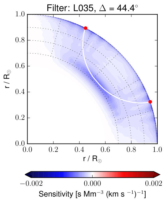 Figure 1
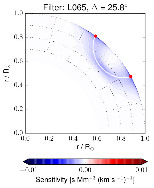 Figure 1
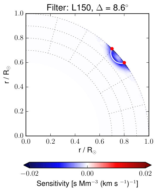 Figure 1
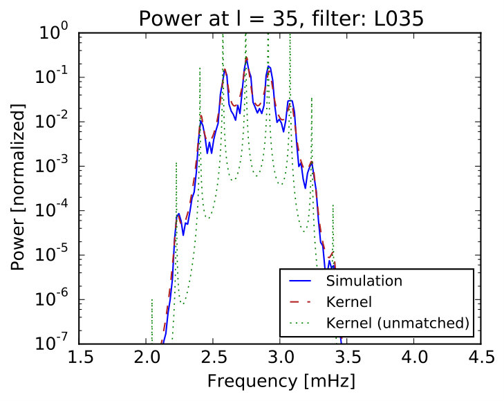 Figure 2
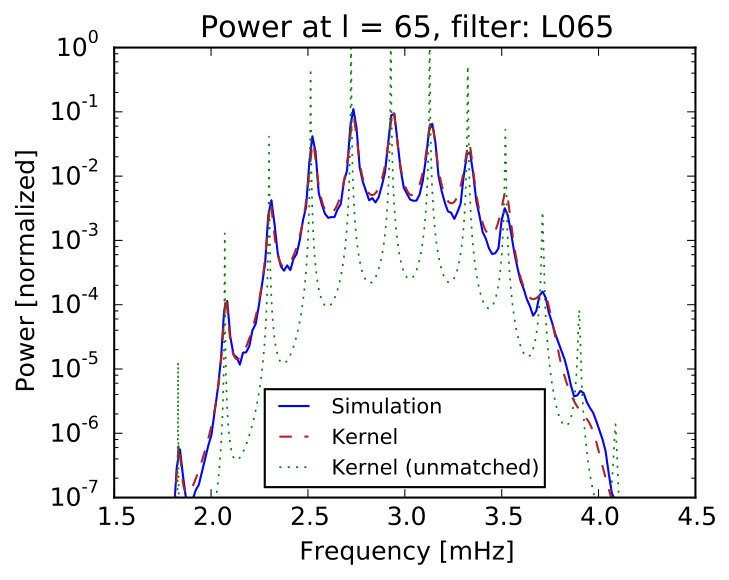 Figure 2
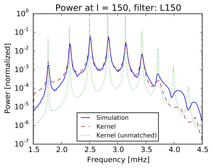 Figure 2
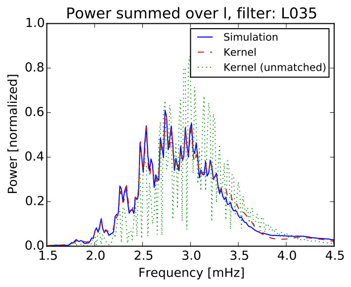 Figure 2
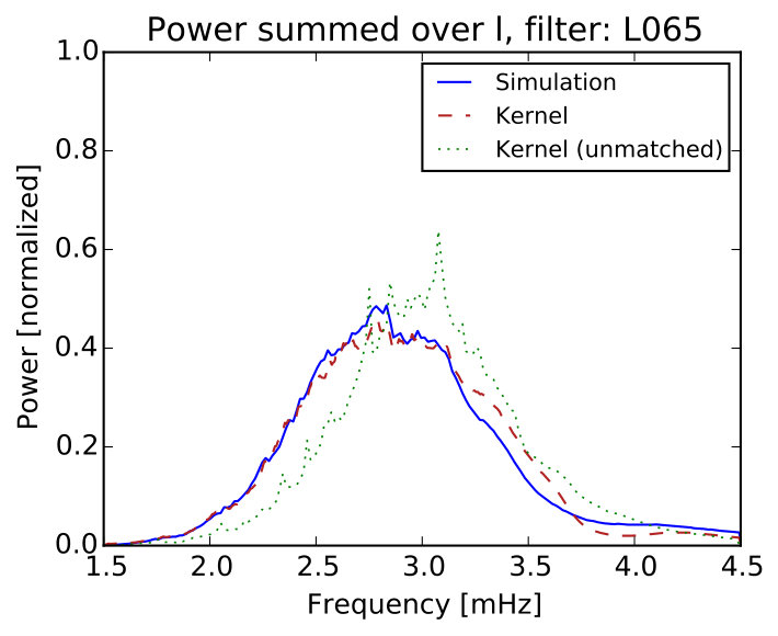 Figure 2
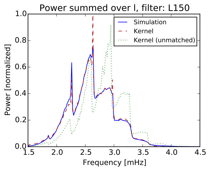 Figure 2
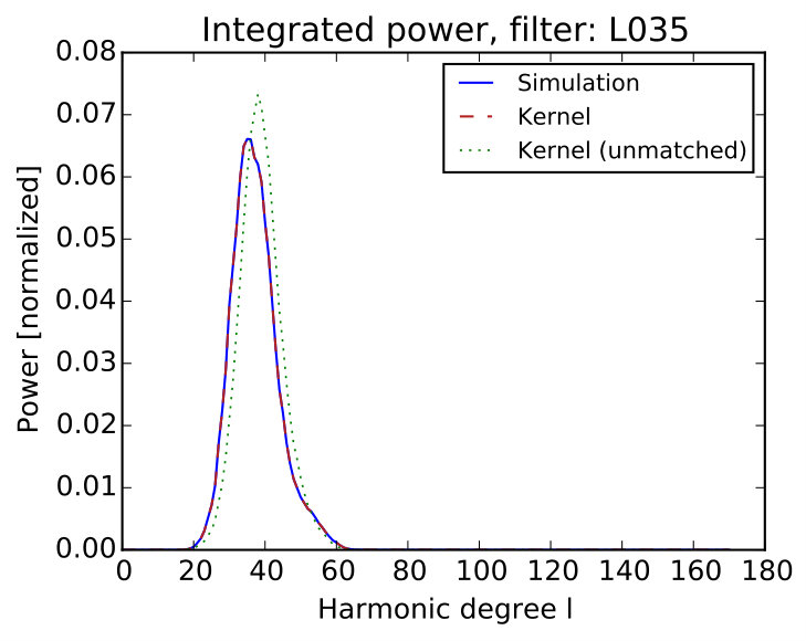 Figure 3
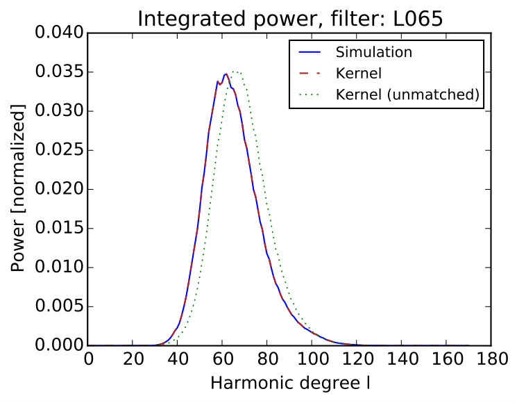 Figure 3
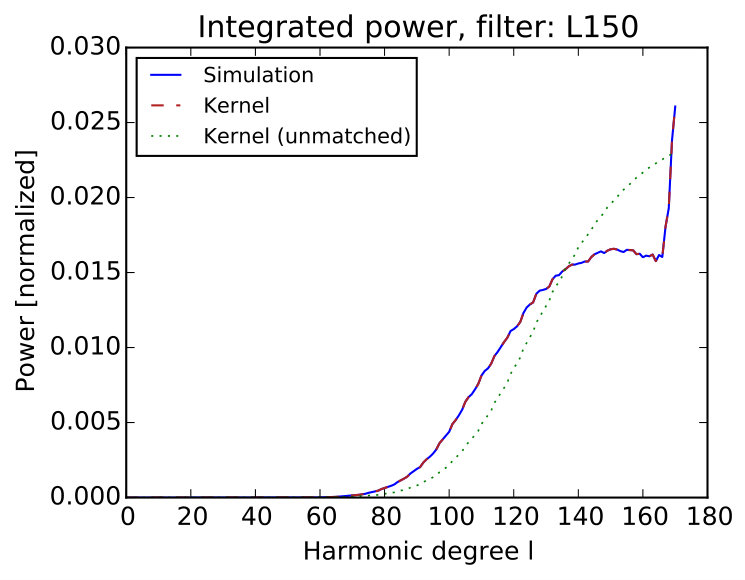 Figure 3
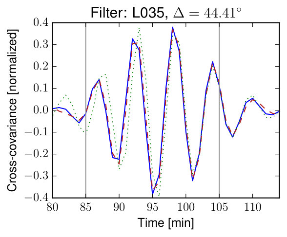 Figure 4
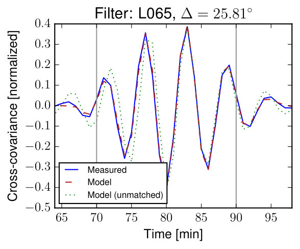 Figure 4
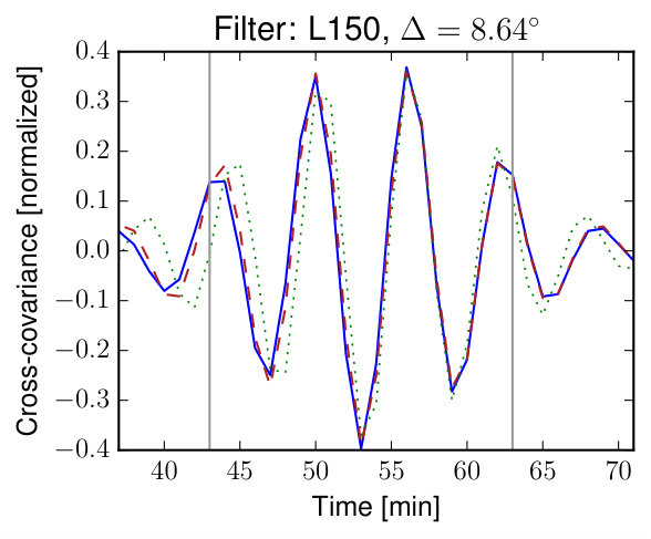 Figure 4
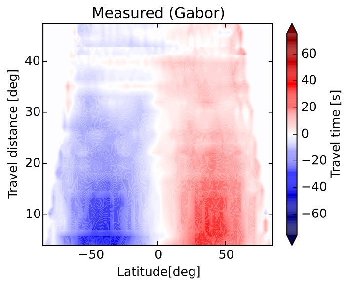 Figure 5
 Figure 5
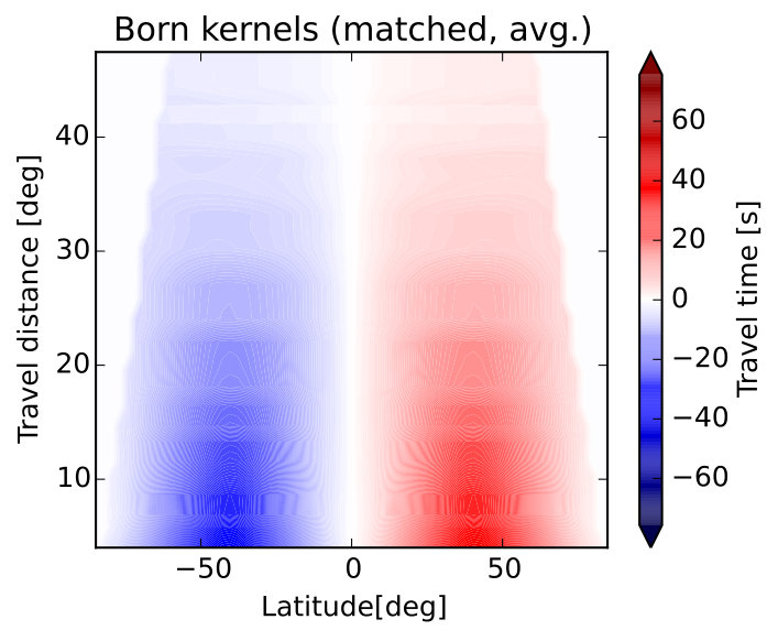 Figure 5
 Figure 5
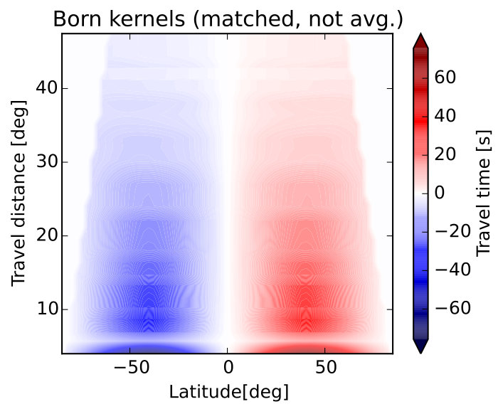 Figure 5
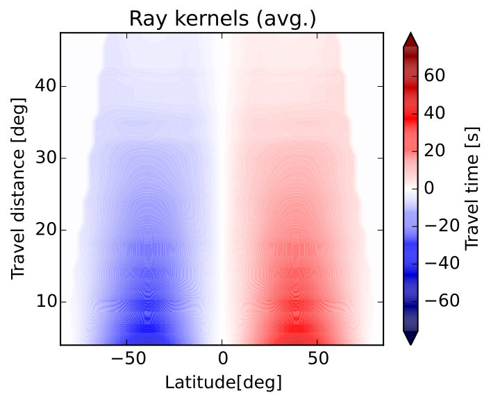 Figure 5
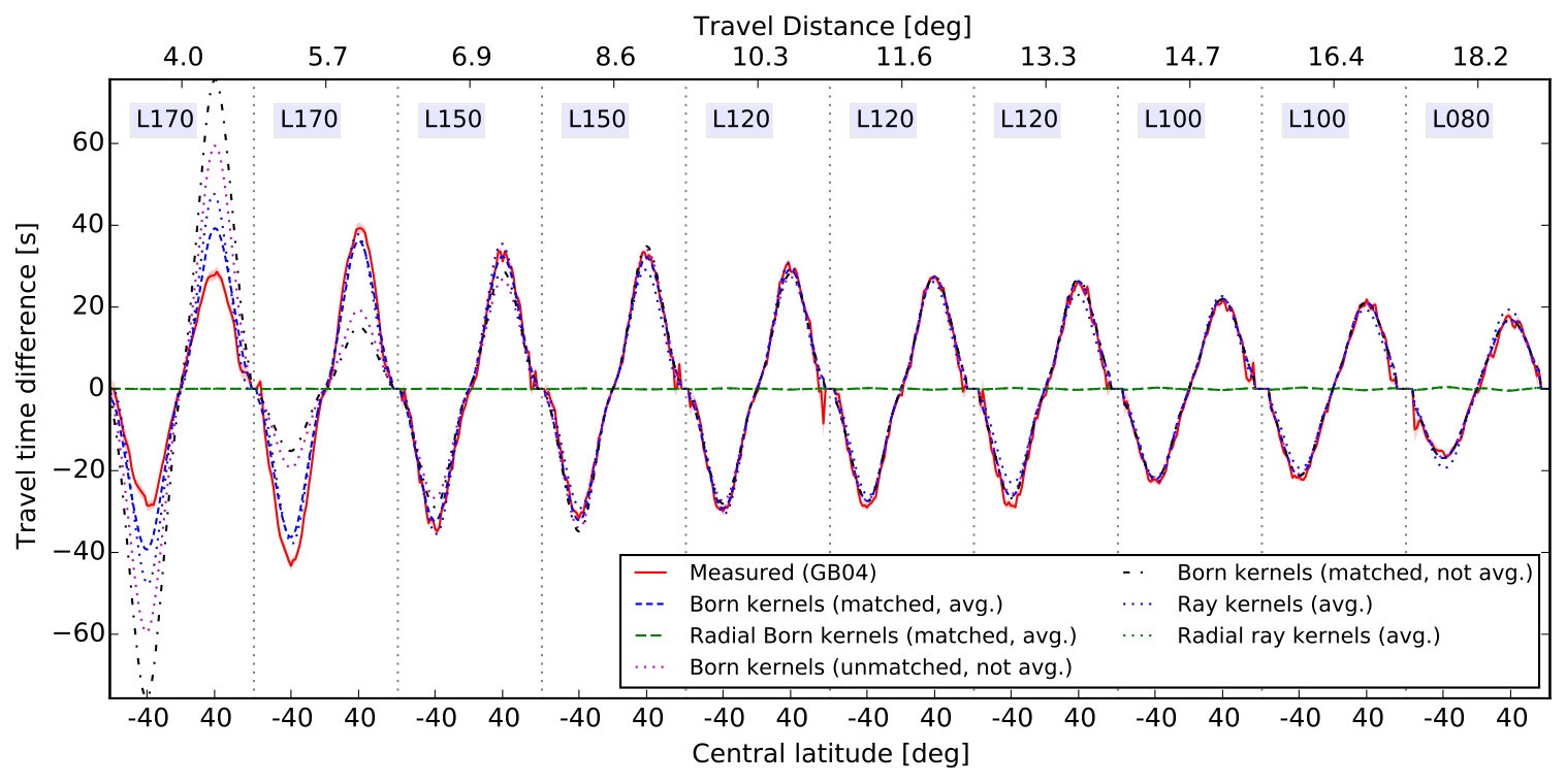 Figure 6
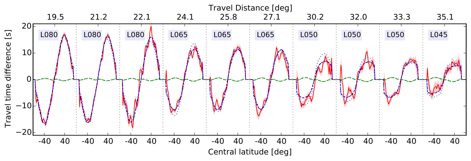 Figure 6
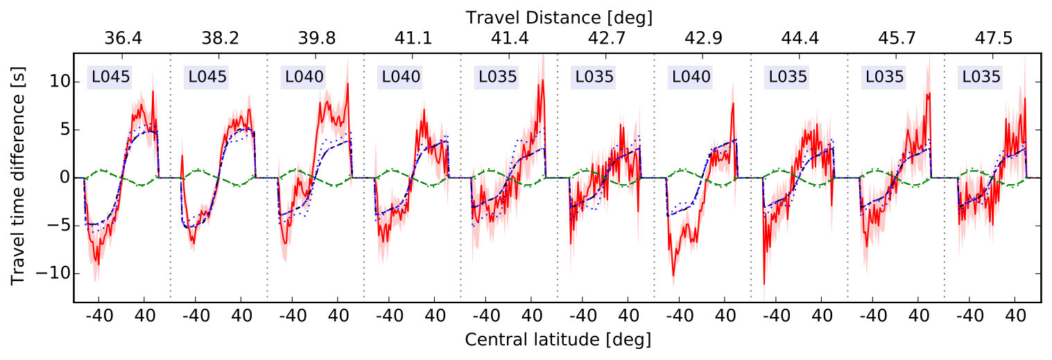 Figure 6
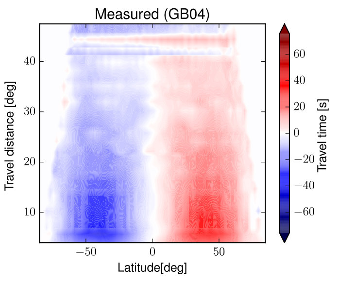 Figure 7
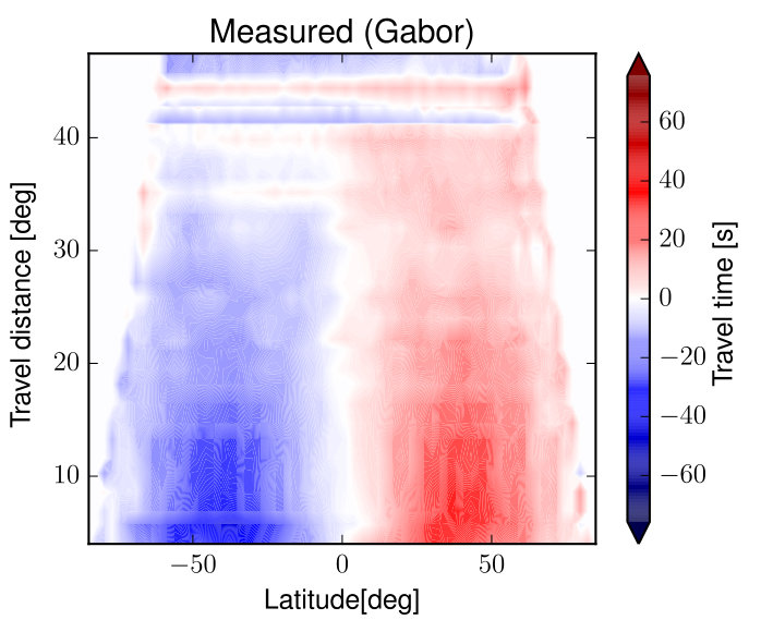 Figure 7
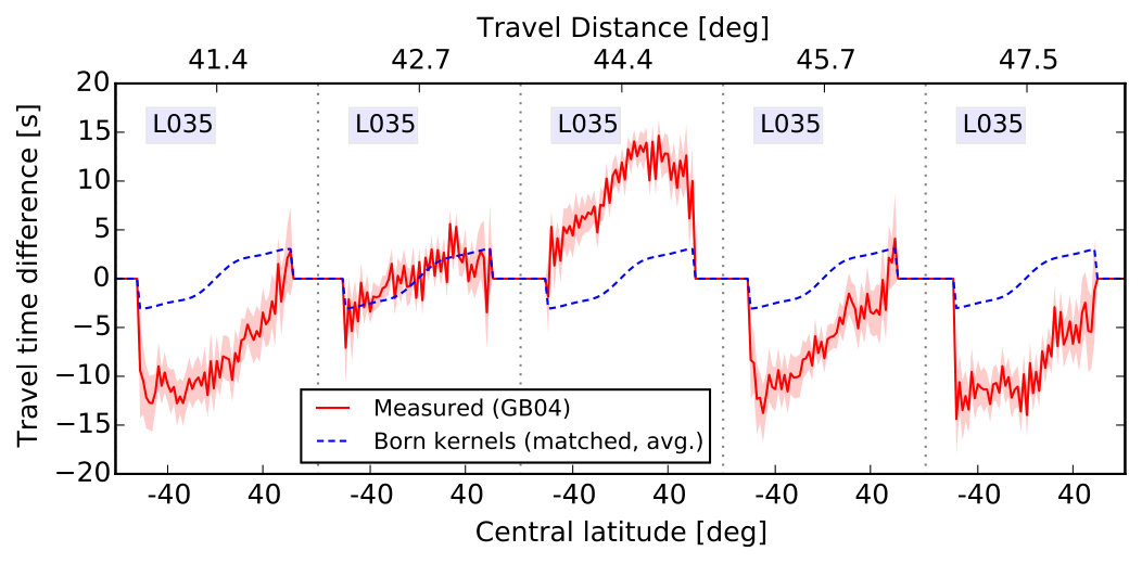 Figure 7
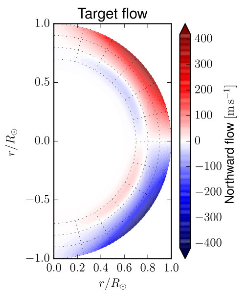 Figure 8
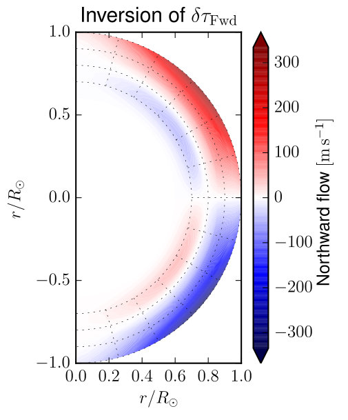 Figure 8
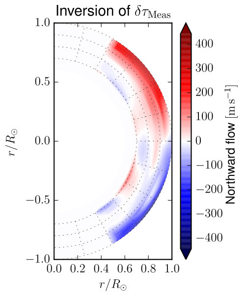 Figure 8
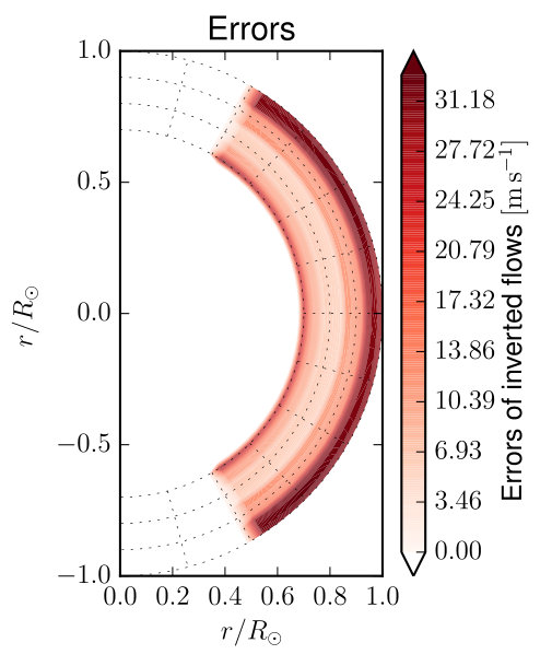 Figure 8
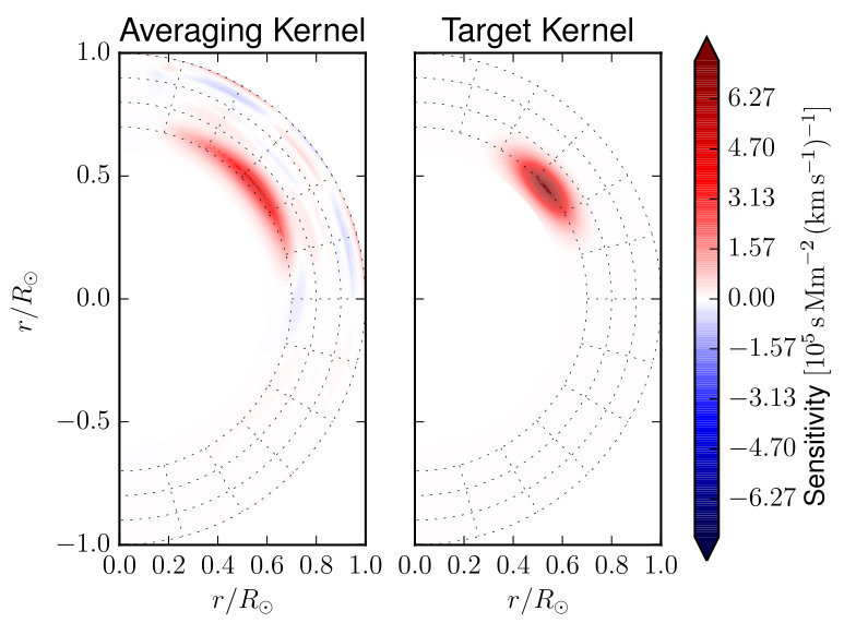 Figure 9
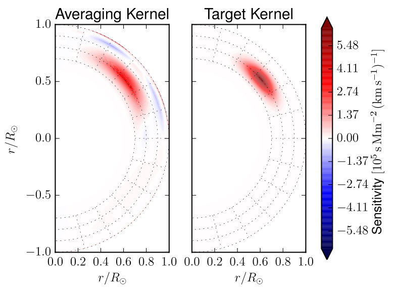 Figure 9
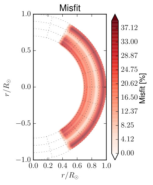 Figure 9
| Matched P. | Unmatched P. | ||||
|---|---|---|---|---|---|
| Filter | Mean | Mean | Mean | Mean | |
| L035 | 342.9 | 2.93 | 37.2 | 3.05 | 38.9 |
| L040 | 308.5 | 2.93 | 41.5 | 3.05 | 43.4 |
| L045 | 274.6 | 2.93 | 46.7 | 3.05 | 49.0 |
| L050 | 248.8 | 2.92 | 51.8 | 3.05 | 54.5 |
| L065 | 199.4 | 2.91 | 65.1 | 3.05 | 69.0 |
| L080 | 158.7 | 2.90 | 82.8 | 3.05 | 88.5 |
| L100 | 130.7 | 2.87 | 101.0 | 3.04 | 108.9 |
| L120 | 106.9 | 2.78 | 121.5 | 2.96 | 130.1 |
| L150 | 78.5 | 2.63 | 138.8 | 2.81 | 143.9 |
| L170 | 30.5 | 2.16 | 157.3 | 2.24 | 156.4 |
Peer Reviews
No public reviews on file for this paper yet. If you reviewed it on a platform where reviews are public (OpenReview, ICLR, NeurIPS, ICML), you can paste yours below so the community can read it here.
Videos
No videos yet. Explain this paper in a talk, walkthrough, or lecture? Add one.
Validation of Spherical Born Approximation Sensitivity Functions for Measuring Deep Solar Meridional Flow
Vincent G. A. Böning
Kiepenheuer-Institut für Sonnenphysik, 79104 Freiburg, Germany
Markus Roth
Kiepenheuer-Institut für Sonnenphysik, 79104 Freiburg, Germany
Jason Jackiewicz
New Mexico State University, Las Cruces, NM 88001, USA
Shukur Kholikov
National Solar Observatory, Tucson, AZ 85719, USA
Abstract
Accurate measurements of deep solar meridional flow are of vital interest for understanding the solar dynamo. In this paper, we validate a recently developed method for obtaining sensitivity functions (kernels) for travel-time measurements to solar interior flows using the Born approximation in spherical geometry, which is expected to be more accurate than the classical ray approximation. Furthermore, we develop a numerical approach to efficiently compute a large number of kernels based on the separability of the eigenfunctions into their horizontal and radial dependence. The validation is performed using a hydrodynamic simulation of linear wave propagation in the Sun, which includes a standard single-cell meridional flow profile. We show that, using the Born approximation, it is possible to accurately model observational quantities relevant for time-distance helioseismology such as the mean power spectrum, disc-averaged cross-covariance functions, and travel times in the presence of a flow field. In order to closely match the model to observations, we show that it is beneficial to use mode frequencies and damping rates which were extracted from the measured power spectrum. Furthermore, the contribution of the radial flow to the total travel time is found to reach 20% of the contribution of the horizontal flow at travel distances over . Using the Born kernels and a 2D SOLA inversion of travel times, we can recover most features of the input meridional flow profile. The Born approximation is thus a promising method for inferring large-scale solar interior flows.
Subject headings:
scattering — Sun: helioseismology — Sun: interior — Sun: oscillations — waves
††slugcomment: To appear in the Astrophysical Journal.
1. INTRODUCTION
Accurate inferences of solar meridional flow are important for modelling the solar dynamo (e.g., Charbonneau, 2014, Charbonneau, 2010). At or near the surface, the magnitude of the meridional flow is known to a good extent (e.g., Gizon and Birch, 2005, Miesch, 2005) from a variety of methods such as Doppler-shifts and feature tracking (e.g., Ulrich, 2010; Hathaway, 2012), time-distance helioseismology (e.g., Giles et al., 1997; Beck et al., 2002; Zhao and Kosovichev, 2004,) ring-diagram analysis (e.g., Haber et al., 2002; Komm et al., 2005; González Hernández et al., 2008, 2010; Basu and Antia, 2010), and Fourier-Hankel analysis (Braun and Fan, 1998; Krieger et al., 2007).
The nature of meridional flows in deeper layers below about 0.9 solar radii still remains under debate. Such measurements were obtained using tracking of supergranules (Hathaway, 2012) and helioseismologic techniques, such as time-distance helioseismology (Giles et al., 1997; Zhao et al., 2013; Jackiewicz et al., 2015; Rajaguru and Antia, 2015), Fourier-Hankel analysis (Braun and Fan, 1998), and global helioseismology (Schad et al., 2013). The conclusions on the global pattern of the meridional flow are very different, ranging from multiple cells in depth (Zhao et al., 2013) and multiple cells in depth and latitude (Schad et al., 2013) to a single-cell picture with a return flow starting in rather shallow layers (Jackiewicz et al., 2015; Hathaway, 2012, at about 0.9 solar radii) or in deeper regions (Giles et al., 1997; Braun and Fan, 1998; Rajaguru and Antia, 2015, below 0.85 solar radii). However, there are several details to keep in mind concerning these inversion results (Jackiewicz et al., 2015), e.g., that uncertainties in the results due to systematic effects are likely to be larger than the random errors in the inversion results, that the results were obtained using different instruments, and that they cover different periods in time. Furthermore, the impact of the radial flow component on the travel times was not taken into account in the results obtained by Zhao et al. (2013) and Jackiewicz et al. (2015).
In time-distance helioseismology (Duvall et al., 1993), flows can be inferred using sensitivity functions (kernels), which are a model for the impact of the flows on travel-time measurements of acoustic waves. Measurements of deep meridional flow have so far been done using the rather classical ray approximation (Kosovichev, 1996; Kosovichev and Duvall, 1997). In this model, travel times are assumed to be sensitive to flows only along an infinitely thin ray path which connects the two observation points.
Recently, Böning et al. (2016) extended a Born approximation model for the travel-time measurements from Cartesian to spherical geometry. An alternative approach for computing Born kernels was proposed very recently by Gizon et al. (2016). These developments permit the use of Born approximation kernels for inferring the deep meridional flow. In the Born approximation (e.g., Birch and Kosovichev, 2000, Gizon and Birch, 2002), the full wave field in the solar interior is modelled using a damped wave equation which is stochastically excited by convection. This wave equation is solved in zero-order and in its first-order perturbation, which includes advection in the presence of a flow field. When modelling travel times using the Born approximation, the advection and first-order scattering of the wave field at any location inside the Sun is thereby taken into account.
The ray approximation is expected to be accurate if the underlying flow field does not vary at length scales which are smaller than a wavelength (e.g., Birch et al., 2001). In the case of flows at the bottom of the convection zone, this scale was estimated to be of the order of (Böning et al., 2016 and references therein). If the flow varies on smaller length scales, the Born approximation is thought to be more accurate (e.g., Bogdan, 1997, Birch and Felder, 2004, Couvidat et al., 2006, and Birch and Gizon, 2007).
In addition to modelling the perturbation to the full wave field in the solar interior, an advantage of the Born approximation is that it also provides a model for additional observational quantities, such as disc-averaged cross-covariances and mean power spectra, which is not the case for the ray approximation. The accuracy of the model can therefore easily be validated.
Several methods for inferring the deep solar meridional flow (Zhao et al., 2013; Jackiewicz et al., 2015; Roth et al., 2016) have been validated using a linear numerical simulation of the solar interior wave field by Hartlep et al. (2013), which includes a standard single-cell meridional flow profile. The same simulation is to be used in this paper in order to validate the use of spherical Born kernels for inferring solar meridional flows.
In Section 2, we will give a short introduction to the Born approximation as used in time-distance helioseismology. Section 3 includes the details of a numerical optimization, which was necessary in order to obtain the required number of kernels in an acceptable amount of time. The main comparison of the Born approximation model with artificial data obtained from the simulation is presented in Section 4. In Section 5, we discuss the relevance of the radial flow component on the measured travel times. Furthermore, we show inversion results of this data obtained with the Born kernels in Section 6. Conclusions are presented in Section 7.
2. THE BORN APPROXIMATION IN TIME-DISTANCE HELIOSEISMOLOGY
We first briefly summarize the Born approximation model introduced by Böning et al. (2016), which is to be validated in the following sections. Following Gizon and Birch (2002), the measurement process in time-distance helioseismology is modelled as closely to observations as possible. The objective of the model is to give a linear relationship between a small-magnitude flow field in the solar interior, which perturbs a mean observed or background model travel time, , according to
[TABLE]
where denotes the expectation value of a stochastic quantity. Vector quantities are printed in bold throughout this work. Once an expression for the sensitivity function is found and travel times are measured, Equation (1) can be used to infer solar interior flows.
In order to achieve this goal, a model is first developed for an unperturbed spherically symmetric non-rotating Sun (zero-order problem). The stochastically driven and damped wave equation for solar oscillations is solved by expansion into solar eigenmodes. The resulting wave field at location and time can be used to model the observed Doppler signal via , where the line-of-sight is assumed to be radial. After a spherical harmonic transform
[TABLE]
and a Fourier transform (indicating the Fourier transform by the use of the variable instead of ), a power spectrum can be computed both from observations and from the model,
[TABLE]
where the filtered were obtained by multiplying by a filter function . After reconstructing the filtered Dopplergram time series, ,
[TABLE]
cross-covariances are computed by
[TABLE]
which are used for fitting travel-times from observations, see Gizon and Birch (2002), Gizon and Birch (2004, hereafter GB04), and Böning et al. (2016). As our goal is to measure flows, we use travel-time differences , and the terms travel-time and travel-time difference are used interchangeably in this work.
In order to model the effect of a flow field on the travel times, the zero-order model for the mean Sun is perturbed. The flow is assumed to be small and thus only linear effects are taken into account. The perturbation of the flow is introduced in the wave equation by adding an advection term. This first-order wave equation is solved for the perturbation to the wave field, . Taking only first-order terms (i.e. linear terms) into account, this corresponds to modelling the first-order scattering of the modes in the solar interior due to the flow field, see Gizon and Birch (2002). The perturbation to the wave field is then used to obtain the perturbation to the cross-covariance and the travel-time shift according to Equation (1). The result is
[TABLE]
where the last term is identical to the previous term, apart from complex conjugation and exchange of indices 1 and 2. In Equation (6), the sum is taken over all pairs of eigenmodes and the quantities and describe the scattering of mode into mode due to a flow at location , which is propagated to the observation points at the surface. Each mode is identified by its harmonic degree and radial order . See Appendix A for a recap of the definitions of and .
3. FAST COMPUTATION OF SPHERICAL BORN KERNELS
As the numerical evaluation of Equation (6) is quite costly for obtaining an accurate kernel (about 2 days on 32 CPU cores for a three-dimensional kernel covering only about 5 % of the solar volume with a coarse spatial grid), it is necessary to optimize its computation. This requires a little more mathematical detail, which the reader may well skip in order to understand the main results of this paper.
3.1. 3D Kernels
We here propose an approach in which we make use of the separability of the eigenfunctions into a horizontal and a radial dependence. This is a consequence of the separation of variables performed when solving the oscillation equations (e.g., Aerts et al., 2010). The horizontal dependence of the eigenfunction is then also separable from the radial order of the mode. This allows us to rewrite the kernel formula (6) (see Appendix A for details)
[TABLE]
Here, the quantity includes the horizontal dependence of the kernel from . The quantity includes the sum over and , the factor as well as the -dependent factors and the radial dependence from in Equation (6). If is evaluated before the main loop over , , and the spatial grid in Equation (7), the computational burden of the sum over and does not play a considerable role in the total computation time anymore.
In practice, for a given , the number of radial orders to be summed over is about 10 for probing the deep solar interior. The approach presented here thus decreases the computation time by about two orders of magnitude.
Computing a full 3D sensitivity kernel using harmonic degrees and a spatial grid with grid points (, covering depths until and the complete horizontal domain), therefore, takes about 1 day on 8 CPUs. A complete set consists of one kernel per travel distance, which can be reprojected to different latitudes and used to obtain, e.g., kernels for point-to-arc travel times, see examples presented in Figure 1. Computing such a set with 126 kernels as used in Sections 4 - 6 takes about 3 weeks on 96 CPUs.
Very recently, Gizon et al. (2016) developed an alternative approach for computing Born kernels. This approach is based on numerically solving for the Green’s functions for individual modes and individual frequencies. It allows for a rather flexible computation of kernels for different quantities such as sound-speed, density, flows, and damping properties, as well as a possible inclusion of axisymmetric perturbations to the model.
While a detailed comparison of both methods is left to further studies, we consider as an example the computation of the radial solar model case from Table 2 in Gizon et al. (2016) using the frequency resolution from this study (about 92,000 grid points spread over a range of , see also Böning et al., 2016) and 149 modes. This would thus take about eight times longer than using our method. In general, the computation time for our method scales with the number of modes squared, and the method of Gizon et al. (2016) scales with the number of modes times the number of frequency bins used. As a very fine frequency resolution is necessary to adequately sample the frequency domain in the case of deeply-penetrating modes (Böning et al., 2016), our method is thus advantageous for computing kernels for filtered observations of deep flows, and theirs for computing kernels using many modes or a coarser frequency resolution.
3.2. 2D Integrated Kernels
Furthermore, it is possible to reach an even greater optimization when computing individual kernels which were integrated over the azimuthal coordinate . For inferring flow fields which are rotationally symmetric such as meridional flow or differential rotation, one can rewrite Equation (1) as
[TABLE]
where the integrated Kernel is defined as
[TABLE]
We thus have
[TABLE]
where is the integral over the -coordinate of the variable in Equation (7).
As the numerical evaluation of the integral of over is independent of the radial coordinate, for each latitude, the integration over and the loop over the radius become independent. As a consequence, the computation of an integrated kernel scales with the maximum of the number of radial and azimuthal grid points rather than with their product. For the example presented in Section 3.1, the computation of an integrated 2D kernel is thus about 75 times faster compared to its 3D version. A drawback of this approach, however, is that 2D integrated kernels cannot be projected to different latitudes due to the nature of the coordinate system used. Therefore, this approach turns out to be advantageous if a smaller number of kernels is to be computed.
3.3. Point-to-Arc and other Geometries
It is possible to extend the previous approach for computing 2D integrated kernels to the case of travel times which were averaged over multiple points, e.g. in a point-to-arc geometry, if all individual point-to-point measurements were obtained for the same travel distance . Indicating with and averages of and over all pairs of observation points, we have
[TABLE]
4. BORN APPROXIMATION FORWARD MODEL COMPARED TO SIMULATED DATA
In the following, we use a numerical simulation of helioseismic wave propagation in the solar interior by Hartlep et al. (2013), which includes a standard single-cell meridional flow profile and which has been used before for validation purposes (see Hartlep et al., 2013, Jackiewicz et al., 2015, Roth et al., 2016, and references therein). As explained in Hartlep et al. (2013), the flow was amplified by a factor of about 36 to a maximum amplitude of in order to increase the signal-to-noise ratio. As the simulation is linear, this increase does not alter the physics.
The radial displacement of the oscillations in the simulation at are used as Dopplergrams. They are our input artificial data. Power spectra, cross-covariance functions, and travel times were obtained from this artificial data by Jackiewicz et al. (2015) using a time-distance measurement technique with phase-speed filters (Kholikov et al., 2014). In the following, these observational quantities are compared to the zero- and first-order models to be validated in this paper.
4.1. Power Spectra
Filtered power spectra obtained from the simulation and from the zero-order model are compared in Figures 2 and 3. Figure 2 shows cuts through the power spectra at the central harmonic degree of each filter (top) and power spectra summed over harmonic degree (bottom). Figure 3 shows power spectra integrated over frequency. See Table 1 for details on the filters used.
In the following, the simulated data is compared to our model using two different sets of mode frequencies and damping rates. As a first-guess case, the zero-order model power spectrum, displayed as a green dotted line, was computed with frequencies from Model S and damping rates from MDI (“unmatched” in the legends appearing in this paper). Damping rates were provided by J. Schou (2006, private communication).
It can be seen that the peaks in the model power spectrum are systematically different from the ones in the simulation. The widths of the peaks are systematically smaller in the model power spectrum and the central frequencies of the peaks differ, especially at frequencies above about (best observable in the top right panel). As was discussed in Böning et al. (2016, Section 3.3), the shape of a cut through the model power spectrum matches a Lorentzian function centered at the input mode frequency and with the damping rate as its half width at half maximum. The difference in the location and shape of the peaks between simulation and model thus shows that the mode frequencies and damping rates from the simulated data are different from Model S frequencies and observed damping rates.
As the computation of sensitivity functions is strongly dependent on accurately modelling the data power spectra (e.g., Gizon and Birch, 2002; Birch and Felder, 2004; Jackiewicz et al., 2007; DeGrave et al., 2014a, b), with real solar observations, one would use mode frequencies and damping rates as close to solar values as possible. In order to achieve a good match between model and data power spectra for the validation presented in this paper, we therefore fitted frequencies and damping rates to the simulated power spectrum. These fitted values were used as parameters for the zero-order power spectrum shown as a red dashed curve in Figures 2 and 3 (“matched” in the legends). It can be seen that both the locations and the widths of the peaks of the simulated and zero-order modelled power spectra now match well (Figure 2, top). The amplitude of each peak, however, is not a free parameter in the zero-order model and therefore cannot be adjusted to the simulation.
Additionally, the source correlation time, a free parameter modelling the sources in Böning et al. (2016), was fine-tuned individually for each matched filtered zero-order model power spectrum in order to obtain a power-weighted mean frequency identical to the one from the simulation. This is necessary for guaranteeing that the mean sensitivity of the kernel is correctly adjusted (Jackiewicz et al., 2007, Böning et al., 2016). In addition, the power spectra for the kernel were corrected by an -dependent factor which accounts for a different behavior of the frequency-integrated power in the simulation and in the zero-order model, see Figure 3. See also Table 1 for a summary of properties for the power spectra obtained with matched and unmatched frequencies and damping rates, for each individual filter used in this work.
In the following, we will compare simulated data to the zero- and first-order models obtained using both sets of frequencies and damping rates.
4.2. Cross-Covariances
Born approximation sensitivity functions in time-distance helioseismology as in Böning et al. (2016), Birch and Gizon (2007), and Gizon and Birch (2002) are obtained for a travel-time fit which involves a reference cross-covariance function.
On the data analysis side, it is advantageous to use some kind of disc- and time-averaged cross-covariance function as a reference. This assures that travel-times measured at individual locations at a certain point in time correspond to local changes compared to the mean solar cross-covariance for a particular travel distance.
On the modelling side, the zero-order cross-covariance function is usually used as a reference function. Figure 4 shows a comparison of these reference cross-covariance functions for different exemplary travel distances. It can be seen that the model fits the data very well once the fitted frequencies and damping rates were used.
4.3. Travel Times
Travel times fitted to the cross-covariances obtained from the simulated data can be compared to forward-modelled travel times, which can be obtained from the Born kernels using Equation (1) or (8) as the underlying flow field is known.
Figures 5 and 6 show a comparison of such travel times. The displayed measured travel-times were obtained by rebinning an original set of travel times for 598 central latitudes and 126 distances to 66 latitudes and 30 distances. The corresponding averaging was applied to the kernels used for the forward travel times marked with “avg.” in Figures 5 and 6. For the forward-modeled travel times marked with “not avg.”, however, the kernels have not been averaged. Instead, we have just computed one center-to-arc kernel for each of the 66 times 30 distances. Furthermore, we also show forward travel-times from kernels obtained with an unmatched power spectrum.
In Figure 5, it can be seen that the travel times from the kernels generally fit very well to the measured ones. The forward-modelled travel times, which were obtained using properly averaged Born kernels and a matched power spectrum (top right panel), also reproduce some of the jumps visible in the measured travel times as a function of distance at mid-latitudes. These jumps are introduced by a change of phase speed from filter to filter. It can also be seen that there do not seem to be significant differences between the Gabor and GB04 fits.
Horizontal cuts through the panels displayed in Figure 5 are shown in Figure 6, where the match between forward-modelled and measured travel times can be inspected in more detail. It can be seen that forward-modelled travel times fit the measured ones within the measurement errors for most distances. The agreement is particularly good for travel distances of about 8-20 degrees with measurement errors increasing with increasing travel distance.
At very low travel distances (about ), it can be seen that the forward-modelled travel times do not fit the measured ones. The reason for this effect lies in the fact that the simulated data only incorporates modes with harmonic degree . This cut-off acts as an additional filter at a harmonic degree at which the filter with the lowest phase speed (L170) is centered. The modes selected by the filter thus do not form a proper wave packet, which may lead to artifacts in the cross-correlations (see, e.g., Zharkov et al., 2006).
Additionally, it is noteworthy that the quality of the match of the power spectrum (compare matched vs. unmatched) does not have a large effect on the travel times at higher travel distances (). At smaller travel distances (), however, one can observe a substantial effect of the quality of the match of the power spectrum on the travel times. We note here that this conclusion may be different for other flow models. We also note that the absence of a proper averaging of multiple kernels in distance and latitude has a considerable effect for smaller travel distances () but seems to vanish for the largest distances in the case of the flow model considered here.
For comparison, forward travel times using ray kernels are also shown in Figures 5 and 6. It can be seen that the magnitude of the ray kernel travel times is, in general, very similar to those obtained using Born kernels. However, Born kernels seem to better reproduce some features in the measured travel times, e.g., jumps in the magnitude of the travel times from one filter to another such as from to (see the middle panel in Figure 6). As the given flow model varies on rather large length scales, a relatively good performance of the ray kernels is expected. This may be different for meridional flow models which vary on smaller length scales, see Section 1.
We also note here that the measured travel times obtained using the filter with the highest phase speed (L035) encounter a spurious constant offset, see Figure 7. This offset was corrected for by substracting the mean travel time at each distance. Such an offset is not present in real solar data (Kholikov et al., 2014, Jackiewicz et al., 2015). In Jackiewicz et al. (2015), this offset was not noticed in the simulated data, as a few distances had been dropped from the analysis, which resulted in an equivalent correction. The origin of this offset is not completely understood but may be connected to the relatively coarse spatial resolution of the simulated data (256 pixels on 180 degrees).
5. IMPACT OF THE RADIAL FLOW COMPONENT
As the influence of the radial flow component on the travel times has not been taken into account by Zhao et al. (2013) and Jackiewicz et al. (2015), we evaluate its impact in the following using our Born approximation model, see the green dashed line in Figure 6. For small travel distances, the contribution from the radial flow to the total travel time is small and increases with travel distance. E.g., for a latitude of and a travel distance of , the impact of the radial flows relative to the horizontal flows is . This ratio increases to for a travel distance of . However, for all distances, the magnitude of the contribution of the radial flows is smaller than the measurement errors of the travel times.
This result is valid for the special case of the simulated data and the flow profile used in this study. Nevertheless, it indicates that it may be worthwhile to study the impact of including kernels for the radial flow component in meridional flow inversions.
6. OUTLOOK: INVERSIONS WITH BORN KERNELS
In order to show that spherical Born approximation kernels can be used for inferring solar meridional flows, a standard SOLA inversion procedure for the horizontal flow component is carried out following the approach of Jackiewicz et al. (2015) using only the horizontal component of the Born kernels.
The travel times for the two smallest travel distances belonging to the lowest phase-speed filter (L170) were excluded from the inversion as they cannot be trusted, see the discussion in Section 4.3 and Figure 6.
In Figure 8, the inversion results are shown. The target flow profile (first panel) was obtained by convolving the target kernels with the flow profile from the simulation. The second panel shows a flow map resulting from the inversion of noiseless forward-modelled travel times. It can be seen to match qualitatively very well the target flow profile. The inversion result for the noisy measured travel times (third panel) matches the target flow in a coarser sense, recovering some but not all of the flow pattern from the simulation.
Figure 9 shows averaging and target kernels for two example target locations. The misfit of the averaging kernels shown in the right panel of Figure 9 was obtained with
[TABLE]
where is the averaging kernel and is the target kernel for a particular target location . We note that the weights and thus the averaging kernels are identical for both inversions presented here.
7. CONCLUSIONS
In this paper, we have presented the validation of spherical Born kernels for inferring the deep solar meridional flow with time-distance helioseismology.
We showed that it is possible to efficiently compute spherical Born kernels for measuring the deep solar meridional flow. To do so, we used the recently developed approach of Böning et al. (2016), which was further optimized for computational efficiency, either for obtaining two-dimensional integrated or full three-dimensional kernels. The numerical optimization was based on the horizontal variation of the eigenfunctions being separable from the radial dependence and the radial order of the mode. Compared to a recently developed method by Gizon et al. (2016), the numerical efficiency of our method is found to be similar, with some advantages in the case of filtered kernels or in the case of a fine frequency resolution as needed for deep flow measurements.
Using a spherical Born approximation model, it is possible to accurately model observational quantities relevant for time-distance helioseismology such as the mean power spectrum, disc-averaged cross-covariances, and first-order travel times perturbed by a given flow field.
We also show that the match of the reference cross-covariance between model and observations depends on the match of the model power spectrum to the observed one. The agreement is very good if the mode frequencies and damping rates entering the model are extracted from the measured power spectrum. The match between observed and modelled travel times, however, does not seem to depend significantly on the match in the power spectrum for travel distances larger than for the flow model considered here. For travel distances smaller than , we found a noticeable dependence of the forward travel times on the match of the power spectrum to observations.
Using a standard 2D SOLA inversion of travel times measured from the simulated data for the horizontal flow component, we can recover most features of the input meridional flow profile in the inverted flow map. The agreement is particularly good for the inversion of noiseless forward-modelled travel times. When inverting noisy measured travel times, we obtain a coarse agreement between inverted and target flows. This shows that Born kernels can be used for inferring the deep solar meridional flow if the noise level in the data is small enough.
The Born approximation is thus a promising method for inferring large-scale solar interior flows. We note, however, that an extensive study is needed in order to compare the use of Born and ray kernels in inversions of the deep meridional flow in more detail.
Acknowledgements: The research leading to these results has received funding from the European Research Council under the European Union’s Seventh Framework Programme (FP/2007-2013) / ERC Grant Agreement n. 307117. This work was supported by the SOLARNET project (www.solarnet-east.eu), funded by the European Commission’s FP7 Capacities Programme under the Grant Agreement 312495. J.J. acknowledges support from the National Science Foundation under Grant Number 1351311. S.K. was supported by NASA’s Heliophysics Grand Challenges Research grant 13-GCR1-2-0036. The authors thank Thomas Hartlep for providing the simulated data. V.B. thanks Kolja Glogowski for computing eigenmodes for Model S and helping with many science-related IT issues. The authors acknowledge fruitful discussions during the international team meeting on “Studies of the Deep Solar Meridional Flow” at ISSI (International Space Science Institute), Bern. The authors thank the referee for constructive comments which improved the paper.
Appendix A FAST COMPUTATION OF SPHERICAL BORN SENSITIVITY FUNCTIONS
Our starting point is from Equations (38-40) in Böning et al. (2016),
[TABLE]
where
[TABLE]
It is now possible to separate the horizontal and radial dependence of the eigenfunctions imprinted in the operators in Equation (A2) (see Böning et al., 2016, Eq. (17), for their definition) so that one obtains
[TABLE]
using appropriate definitions for . From Equations (A4) and (6) we derive, bearing in mind ,
[TABLE]
where we defined
[TABLE]
The reference list from the paper itself. Each links out to its DOI / PubMed record.
- 1Charbonneau (2014) P. Charbonneau, ARA&A 52 , 251 (2014) . · doi ↗
- 2Charbonneau (2010) P. Charbonneau, Living Rev. Sol. Phys. 7 , 3 (2010) . · doi ↗
- 3Gizon and Birch (2005) L. Gizon and A. C. Birch, Living Rev. Sol. Phys. 2 , 6 (2005) . · doi ↗
- 4Miesch (2005) M. S. Miesch, Living Rev. Sol. Phys. 2 , 1 (2005) . · doi ↗
- 5Ulrich (2010) R. K. Ulrich, Ap J 725 , 658 (2010) . · doi ↗
- 6Hathaway (2012) D. H. Hathaway, Ap J 760 , 84 (2012) . · doi ↗
- 7Giles et al. (1997) P. M. Giles, T. L. Duvall, P. H. Scherrer, and R. S. Bogart, Nature 390 , 52 (1997) . · doi ↗
- 8Beck et al. (2002) J. G. Beck, L. Gizon, and T. L. Duvall, Jr., Ap JL 575 , L 47 (2002) . · doi ↗