TL;DR
This paper presents a highly optimized GPU implementation of the population annealing algorithm, significantly accelerating Monte Carlo simulations for complex systems like the 2D Ising model, with adaptable features for broader applications.
Contribution
It introduces a GPU-accelerated, optimized version of population annealing with advanced features like automatic temperature adaptation and multi-histogram analysis.
Findings
Speed-ups of several orders of magnitude over CPU implementations
Effective adaptation of temperature steps for improved sampling
Versatility for different spin models, including disordered systems
Abstract
Population annealing is a promising recent approach for Monte Carlo simulations in statistical physics, in particular for the simulation of systems with complex free-energy landscapes. It is a hybrid method, combining importance sampling through Markov chains with elements of sequential Monte Carlo in the form of population control. While it appears to provide algorithmic capabilities for the simulation of such systems that are roughly comparable to those of more established approaches such as parallel tempering, it is intrinsically much more suitable for massively parallel computing. Here, we tap into this structural advantage and present a highly optimized implementation of the population annealing algorithm on GPUs that promises speed-ups of several orders of magnitude as compared to a serial implementation on CPUs. While the sample code is for simulations of the 2D ferromagnetic…
Click any figure to enlarge with its caption.
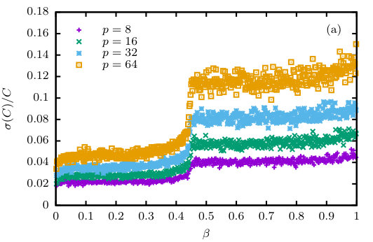 Figure 1
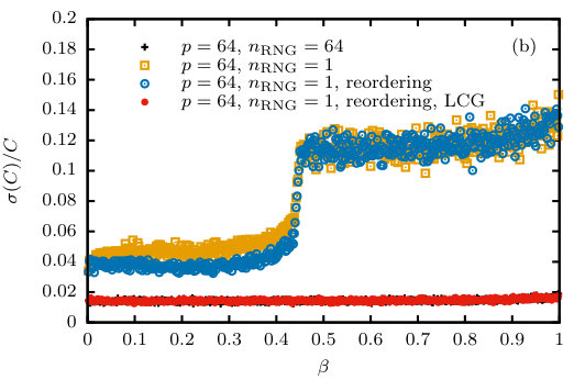 Figure 2
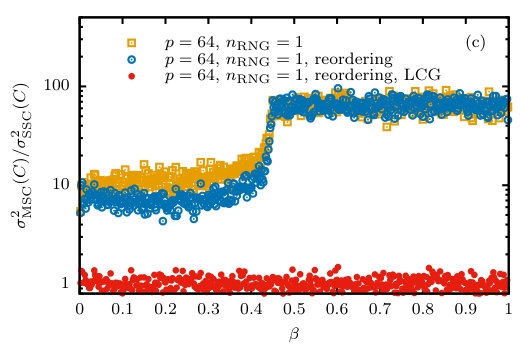 Figure 3
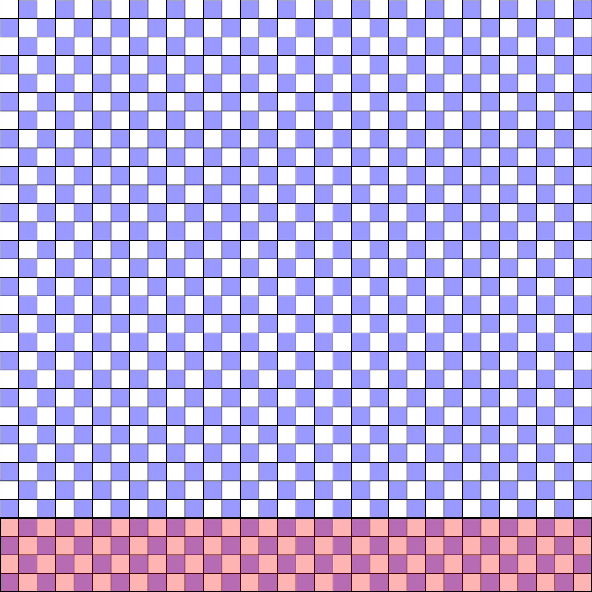 Figure 4
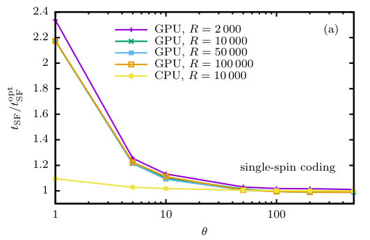 Figure 5
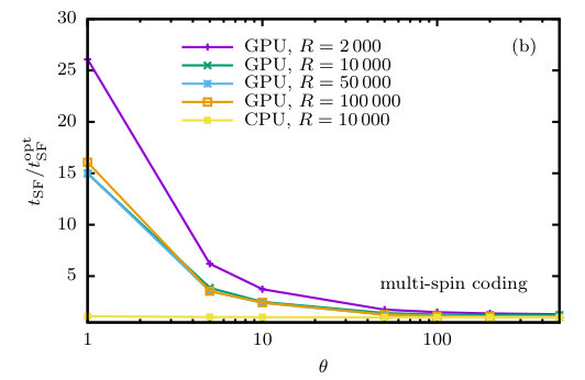 Figure 6
| LCG | speedup | |||
|---|---|---|---|---|
| 8 | 8 | NO | ||
| 16 | 16 | NO | ||
| 32 | 32 | NO | ||
| 64 | 64 | NO | ||
| 8 | 1 | NO | ||
| 16 | 1 | NO | ||
| 32 | 1 | NO | ||
| 64 | 1 | NO | ||
| 8 | 1 | YES | ||
| 16 | 1 | YES | ||
| 32 | 1 | YES | ||
| 64 | 1 | YES |
| CPU | GPU | ||||
| SSC | MSC | ||||
| [ns] | [ns] | speedup | [ns] | speedup | |
| 16 | 23.1 | 0.094 | 246 | 0.0096 | 2406 |
| 32 | 22.9 | 0.092 | 249 | 0.0095 | 2410 |
| 64 | 22.6 | 0.092 | 246 | 0.0098 | 2306 |
| 128 | 22.6 | 0.097 | 233 | 0.0098 | 2306 |
| 256 | 22.5 | 0.098 | 230 | 0.0099 | 2273 |
| 2 000 | 10 000 | 50 000 | 100 000 | ||
| single-spin coding (SSC) | |||||
| 1 | 0.229 | 0.213 | 0.213 | 0.213 | |
| 5 | 0.123 | 0.119 | 0.119 | 0.120 | |
| 10 | 0.111 | 0.108 | 0.107 | 0.109 | |
| 50 | 0.101 | 0.0994 | 0.0985 | 0.0987 | |
| 100 | 0.0998 | 0.0976 | 0.0977 | 0.0975 | |
| 200 | 0.0997 | 0.0972 | 0.0970 | 0.0970 | |
| 500 | 0.0991 | 0.0971 | 0.0969 | 0.0969 | |
| multi-spin coding (MSC) | |||||
| 1 | 0.2504 | 0.1439 | 0.1440 | 0.1543 | |
| 5 | 0.0596 | 0.0372 | 0.0341 | 0.0341 | |
| 10 | 0.0359 | 0.0240 | 0.0232 | 0.0234 | |
| 50 | 0.0168 | 0.0136 | 0.0123 | 0.0121 | |
| 100 | 0.0144 | 0.0123 | 0.0110 | 0.0108 | |
| 200 | 0.0132 | 0.0119 | 0.0103 | 0.0101 | |
| 500 | 0.0125 | 0.0118 | 0.0098 | 0.0097 | |
| 2 000 | 10 000 | 50 000 | 100 000 | ||
| single-spin coding (SSC) | |||||
| 1 | 39.8% | 41.8% | 42.2% | 42.2% | |
| 5 | 76.4% | 77.9% | 78.3% | 78.3% | |
| 10 | 86.6% | 87.6% | 88.0% | 87.9% | |
| 50 | 97.0% | 97.3% | 97.4% | 97.3% | |
| 100 | 98.5% | 98.6% | 98.7% | 98.6% | |
| 200 | 99.2% | 99.3% | 99.3% | 99.3% | |
| 500 | 99.7% | 99.7% | 99.7% | 99.7% | |
| multi-spin coding (MSC) | |||||
| 1 | 5.3% | 6.6% | 5.9% | 5.4% | |
| 5 | 20.6% | 28.7% | 25.1% | 24.4% | |
| 10 | 33.9% | 44.5% | 37.3% | 35.9% | |
| 50 | 71.8% | 80.0% | 75.5% | 76.1% | |
| 100 | 83.6% | 89.0% | 86.7% | 86.3% | |
| 200 | 91.0% | 94.1% | 93.2% | 92.9% | |
| 500 | 96.2% | 97.8% | 97.3% | 97.1% | |
| [ns] | ||||||
|---|---|---|---|---|---|---|
| 1 | 5 | 10 | 50 | 100 | 500 | |
| standard | 0.213 | 0.119 | 0.107 | 0.099 | 0.098 | 0.097 |
| hybrid | 1.424 | 0.361 | 0.232 | 0.126 | 0.112 | 0.101 |
Peer Reviews
No public reviews on file for this paper yet. If you reviewed it on a platform where reviews are public (OpenReview, ICLR, NeurIPS, ICML), you can paste yours below so the community can read it here.
Code & Models
Videos
No videos yet. Explain this paper in a talk, walkthrough, or lecture? Add one.
GPU accelerated population annealing algorithm
Lev Yu. Barash
Martin Weigel
Michal Borovský
Wolfhard Janke
Lev N. Shchur
Landau Institute for Theoretical Physics, 142432 Chernogolovka, Russia
Science Center in Chernogolovka,142432 Chernogolovka, Russia
Applied Mathematics Research Centre, Coventry University, Coventry, CV1 5FB, United Kingdom
P.J. Šafárik University, Park Angelinum 9, 040 01 Košice, Slovak Republic
Institut für Theoretische Physik, Universität Leipzig, Postfach 100920, 04009 Leipzig, Germany
National Research University Higher School of Economics, 101000 Moscow, Russia
Abstract
Population annealing is a promising recent approach for Monte Carlo simulations in statistical physics, in particular for the simulation of systems with complex free-energy landscapes. It is a hybrid method, combining importance sampling through Markov chains with elements of sequential Monte Carlo in the form of population control. While it appears to provide algorithmic capabilities for the simulation of such systems that are roughly comparable to those of more established approaches such as parallel tempering, it is intrinsically much more suitable for massively parallel computing. Here, we tap into this structural advantage and present a highly optimized implementation of the population annealing algorithm on GPUs that promises speed-ups of several orders of magnitude as compared to a serial implementation on CPUs. While the sample code is for simulations of the 2D ferromagnetic Ising model, it should be easily adapted for simulations of other spin models, including disordered systems. Our code includes implementations of some advanced algorithmic features that have only recently been suggested, namely the automatic adaptation of temperature steps and a multi-histogram analysis of the data at different temperatures.
††journal: Computer Physics Communications
PROGRAM SUMMARY
Manuscript Title: GPU accelerated population annealing algorithm
Authors: Lev Yu. Barash, Martin Weigel, Michal Borovský, Wolfhard Janke, Lev N. Shchur
Program Title: PAIsing
Journal Reference:
Catalogue identifier:
Licensing provisions: Creative Commons Attribution license (CC BY 4.0)
Programming language: C, CUDA
Computer: System with an NVIDIA CUDA enabled GPU
Operating system: Linux, Windows, MacOS
RAM: 200 Mbytes
Number of processors used: 1 GPU
Supplementary material:
Keywords: Population annealing; Monte Carlo simulation; Ising model; Parallel computing; GPU; Multi-spin coding
Classification: 23
External routines/libraries: NVIDIA CUDA Toolkit 6.5 or newer
Subprograms used:
*Nature of problem: *The program calculates the internal energy, specific heat, several magnetization moments, entropy and free energy of the 2D Ising model on square lattices of edge length with periodic boundary conditions as a function of inverse temperature .
*Solution method: *The code uses population annealing, a hybrid method combining Markov chain updates with population control. The code is implemented for NVIDIA GPUs using the CUDA language and employs advanced techniques such as multi-spin coding, adaptive temperature steps and multi-histogram reweighting.
*Restrictions: *The system size and size of the population of replicas are limited depending on the memory of the GPU device used.
*Unusual features:
Additional comments:
*Code repository at https://github.com/LevBarash/PAising. Running time: For the default parameter values used in the sample programs, , , , , , , a typical run time on an NVIDIA Tesla K80 GPU is 151 seconds for the single spin coded (SSC) and 17 seconds for the multi-spin coded (MSC) program (see Sec. 2 for a description of these parameters).
1 Introduction
Monte Carlo methods are among the core techniques for studying the statics and dynamics of particle systems in classical and quantum physics, in particular for systems in statistical physics [1]. Although for a few problems simple sampling is reasonably efficient, most applications are based on importance sampling techniques. Among them, Markov chain Monte Carlo (MCMC) is by far the most widely used approach in statistical physics. In quantum Monte Carlo, on the other hand, one can evaluate the wave function in a path-integral formulation in imaginary time by a swarm of particles diffusing in configuration space that undergo a sequence of birth-death processes [2]. This is a special case of a procedure more generally known as sequential Monte Carlo [3]. Such procedures have been more reluctantly adopted in statistical physics applications, but they have gained some traction recently, for example in variants of “go with the winners” simulations [4]. In sequential Monte Carlo, configurations are gradually built in possibly biased steps, sequentially accumulating weights that multiply configurations in the final averages. In many applications such weights fluctuate wildly, thus leading to rather unstable results. In the “go with the winners” approaches, configurations are selectively cloned or pruned in accordance with their weight to tame these fluctuations, a procedure often referred to as population control.
One recent approach of this type is the population annealing (PA) algorithm [5, 6]. There, a large number of configurations are prepared in independent equilibrium configurations, for instance at infinite temperature. Each configuration evolves according to a standard MCMC approach at the given temperature. The population is then gradually cooled, and each configuration sequentially builds up a weight depending on its energy at the instant of temperature change. Population control is used to keep weight fluctuations under control. We here focus on a variant where “perfect” population control is used at each temperature step such that all weights remain equal to unity at all times [7]. The approach has been successfully used for equilibrium simulations of spin-glass systems [8, 9, 10], and also for finding ground states in spin glasses and other systems with frustrated interactions [11, 12]. Recently, we have studied the behavior of PA for simulations of the 2D Ising model, analyzing systematically the dependence on the population size and annealing protocol, and proposed a number of improvements [13].
The era of serial computing came to an end in the early 2000s when CPU clock frequencies first hit the “wall” of about 3.5 GHz, beyond which heat dissipation becomes unfeasible with conventional techniques and the power consumption increases too steeply. While Moore’s law [14] predicting an exponential growth of the number of transistors in an integrated circuit continues to hold, the resulting exponential growth of computational power seen for CPUs essentially stopped being an increase of serial performance (for instance through the increase of clock speeds) and now translates into a corresponding increase in the number of parallel cores or other compute units. Thus the comfortable situation where the same old code or, at least, the same old algorithm could be run on more modern hardware with exponentially decreasing run times with every new generation of machine, has come to an end. Instead, it has become necessary to design and implement solutions to our computational problems that scale well up to thousands or maybe even millions of cores [15]. A computational environment that recently proved to be a particularly useful pathway towards massively parallel computing are graphics processing units (GPUs) and similar accelerator devices. They feature a much higher density of actual compute units than CPUs, at the expense of reduced cache memories and control logic units that are mostly useful for accelerating serial and unpredictable loads, and are hence very well suited for the needs of scientific computing [16, 17]. In statistical physics, significant speed-ups have been observed for Ising model simulations with local [18, 19] as well as non-local [20] udpate algorithms; for continuous-spin systems [21, 22]; for spin glasses [21, 23] and random-field models [24]; for Potts systems [25]; for polymers [26] and many other applications.
The PA algorithm that requires the parallel simulation of a population of tens of thousands up to millions of replicas appears to be a perfect match for this new type of computational resource. The quality of approximation increases with population size [9, 13] such that a higher parallel load is clearly advantageous. As we will show below, we observe a GPU speed-up of around 230 times over a serial CPU based code, thus bringing the wall-clock time for typical calculations of the 2D Ising system considered here down to minutes in many cases. For such models with Ising spins, the additional application of multi-spin coding yields a further up to 10-fold speed-up, such that we reach a peak performance of 10 ps per spin flip of the whole PA simulation code, including the resampling and measurement parts. We provide a flexible implementation that can be configured using command-line switches and should be easily adaptable to simulations of related models such as 3D Ising systems, Potts and models, and spin glasses. In extension to the standard PA algorithm, our code also allows for the adaptive choice of inverse temperature steps and an analysis of the simulation results with a multi-histogram approach.
The rest of the paper is organized as follows. In Sec. 2 we summarize the PA algorithm and the extensions employed here. Section 3 discusses our implementation on GPU, while Sec. 4 introduces the program variant that employs multi-spin coding. In Sec. 5 we investigate the performance and reliability of our code. Finally, Sec. 6 contains our conclusions.
2 Algorithm
The population annealing method was first discussed by Iba [5] in the general context of population-based algorithms and later applied to spin glasses by Hukushima and Iba [6]. More recently, Machta [7] used a method that avoids the recording of weight functions through population control in every step. This is the variant we discuss and implement here.
2.1 Population annealing
As outlined above, the approach is a hybrid of sequential algorithm and MCMC that simulates a population of configurations at each time, updating them with MCMC methods and resampling the population periodically as the temperature is gradually lowered. The algorithm can be summarized as follows:
Set up an equilibrium ensemble of independent copies (replicas) of the system at inverse temperature . Typically , where this can be easily achieved. 2. 2.
To create an approximately equilibrated sample at , resample configurations with their relative Boltzmann weight , where
[TABLE] 3. 3.
Update each replica by rounds of an MCMC algorithm at inverse temperature . 4. 4.
Calculate estimates for observable quantities as population averages . 5. 5.
Goto step 2 unless the target inverse temperature has been reached.
If we choose , equilibrium configurations for the replicas can be generated by simple sampling, i.e., by assigning independent, purely random spin configurations to each copy. The resampling process in step 2 can be realized in different ways [6, 7]. Here we use the following approach [11]. For each replica in the population at inverse temperature we draw a random number uniformly in . The number of copies of replica in the new population is then taken to be
[TABLE]
where is renormalized to ensure that the population size stays close to the target value . Here, denotes the largest integer that is less than or equal to (i.e., rounding down). The new population size is . This method requires only a single call to the random number generator for each replica in the current population and leads to very small fluctuations in the total population size. Note that it is possible that , in which case the corresponding replica disappears from the population, while other configurations will be replicated several times. In the standard setup, steps of equal size in inverse temperature are taken, i.e.,
[TABLE]
and is an adjustable parameter. We discuss an adaptive, automatic choice of temperature steps below in Sec. 2.3. In the code presented here, we use sweeps of Metropolis single-spin flip updates to equilibrate each replica in each temperature step. Other updates such as heat-bath dynamics or even non-local cluster moves could be employed easily as well.
Measurements are taken as population averages, and our code produces estimates for the following quantities,
[TABLE]
Here, denotes the configurational energy and the configurational magnetization of replica , and is the number of spins. Additionally, PA provides a natural estimate of the free energy,
[TABLE]
where is the partition function at inverse temperature , for Ising spins and , and is the reweighting factor (1) used in the resampling. From Eqs. (3) and (4) we can also compute the entropy per site via
[TABLE]
2.2 Weighted averages
It was shown in Ref. [7] that one of the strengths of the PA approach is that by combining the data from independent runs not only statistical errors are decreased, but also systematic deviations can be reduced. This is the case if one uses weighted averages of results of independent runs. As was shown in Refs. [7, 9], an unbiased way of combining the results of independent runs of PA for the same system and target population size is to weight them by the free energies as estimated according to Eq. (4),
[TABLE]
with
[TABLE]
where denotes the average of observable in simulation and the corresponding free-energy estimator according to Eq. (4). The concept of weighted averages allows for an additional parallelization in splitting the total simulation into independent parts. The weighting ensures that this does not substantially degrade the quality of the results [9, 13]. Note that the concept of weighted averages is more general than the PA approach [27], but for the present algorithm the necessary free-energy estimates are a free by-product of the simulation according to Eq. (4). In the implementation provided here, multiple runs can be requested on the command line, but the weighted averaging of results is left to the user to perform separately.
2.3 Adaptive temperature steps
While an annealing cycle of the population is valid for any choice of the temperature sequence , , , and given a sufficiently large number of MCMC sweeps employed at each temperature it also leads to essentially unbiased estimates of observables, the resampling step is only effective if is sufficiently small [13]. The optimal size of temperature steps will itself depend on temperature, and a uniform stepping is not in general ideal. As was recently shown in Ref. [13] uniform effectiveness of resampling is achieved by ensuring a constant overlap of the energy histograms of population members between the neighboring temperatures. This overlap can be computed from the reweighting factors before actually performing the resampling step, and one finds
[TABLE]
Clearly, , and one can use numerical root finding techniques such as, for instance, bisection search, to find such that and then set . Values of provide sufficient histogram overlap without an unnecessary proliferation of temperature steps. In practice, if runs are performed for additional averaging, our code used in adaptive mode decides about temperature steps only in the first run and keeps the temperature sequence fixed for the remaining passes.
2.4 Multi-histogram reweighting
As a PA sweep produces samples at a large number of closely spaced temperatures (typically at least 100, even for small systems), it is natural to combine these data to increase the accuracy and reduce statistical fluctuations in the spirit of the multi-histogram analysis of Ferrenberg and Swendsen [27]. Neglecting correlations between the data at different temperatures as well as the effect of autocorrelations, an optimized combination of histograms to yield an estimate of the density of states is given by [13]
[TABLE]
Here, denotes the total number of temperatures, and we assumed a normalization of the histogram at inverse temperature such that . We note that the storage requirements are moderate as at each time one only needs to store the sum of histograms up to the current temperature and not each histogram individually. Generalizations to other quantities such as magnetizations are possible [13].
3 GPU realization
For definiteness we focus on an implementation for the ferromagnetic, zero-field Ising model on the square lattice with Hamiltonian
[TABLE]
Here, interactions are only between nearest neighbors and periodic boundary conditions are assumed. As is well known, this model undergoes a continuous phase transition at the inverse temperature [28]. The question of how well suited population annealing is as a simulation technique to study this model and its transition is discussed in Ref. [13]. Here, we are not concerned with this aspect, but we use this model as a convenient starting point since a wealth of exact or extremely accurate results are available for it as reference points, and a generalization of the code to other spin models and even more general systems such as polymers or particle systems should be rather straightforward.
General considerations
Inspecting the algorithm given in Sec. 2.1, one identifies three computationally demanding steps: a resampling of the population that involves the determination of weight factors and the copying of replicas, the update of individual configurations with MCMC moves (i.e., spin flips), and the measurement of observables. As we shall see below when reporting the performance results, most time (on CPU or GPU) is normally spent on spin flips (see also Ref. [13]), while for typical choices of (, say) the resampling step and the measurements of the elementary quantities listed in Eqs. (3)–(5) are much less time consuming111As we shall see below, however, this balance is somewhat changed for the case of a multi-spin coded implementation.. These observations suggest to also choose the effort for optimization of each of these parts correspondingly. We hence first focus on the spin updates.
One of the basic features of present day GPU devices that is of paramount importance for performance is the technique of latency hiding implemented in the scheduling algorithm [29]. Each time an elementary group of threads (given by a warp of 32 threads on current NVIDIA GPUs) accesses some data in memory that is currently not cached, there is a latency of hundreds or even thousands of clock cycles until the read or write operation completes. Instead of leaving the compute units idle, the scheduler puts the present warp in the queue and allows another warp that has already completed its data transaction to use the compute units. If only enough such thread groups are available, the compute cores will be kept constantly busy and hence the memory latencies are hidden away. Good GPU performance thus requires to break the work into many threads, optimal performance is often only reached for thread numbers in excess of ten times the number of available physical cores [30].
A second crucial requirement for exploiting the full potential of GPUs relates to the minimization of costly global memory accesses. This includes a reasonable level of compression of the data to be transferred for the updates. For the present problem with Ising variables it suggests to use the narrowest available native data type to represent spins, which is an 8-bit integer, or to revert to a multi-spin coding approach. A discussion of the latter technique is postponed until the next section. Further, the relative slowness of memory makes it useful to cache and re-use data as much as possible, which could involve using automatic caches or the user-managed cache known as shared memory [29]. Finally, it implies optimization geared towards increasing the locality of memory operations as each direct access to global memory (implying a cache miss) fetches a full cache line of 128 bytes. Ideally, the threads in a warp access memory locations in the same cache line(s), thus making use of all of the data that is actually loaded. This concept is known as memory coalescence.
Spin updates
By construction population annealing suggests to parallelize the calculations for different members of the population. One particularly simple code setup is hence to assign one thread to the updating of each replica such that in total threads are used for the MCMC part of the algorithm, i.e., for flipping spins. Each thread then goes sequentially through the lattice. To ensure good memory coalescence in this case, the same spins of each replica should be placed next to each other in memory, so configurations should be stored in replica-major order. In practice this code setup, which we denote as replica-parallel, does show good but not optimal performance, especially for smaller population sizes where it does not provide enough parallelism. Where this approach does not provide optimal performance, it still has the advantage of being completely general, and it could consequently be applied unaltered to PA simulations of any other model. We hence mention it here as a safe fall-back solution especially for problems for which it is not possible or straightforward to implement a domain decomposition (for instance for systems with long-ranged interactions).
To increase the amount of parallel work, for the present code for the 2D Ising model we opted to additionally parallelize the updates for each single replica, using a domain decomposition of the lattice. This was extensively used previously for simulations using MCMC (single-spin flips) only. The basic step consists of a checkerboard decomposition of the lattice which allows for independent updates of all spins of one sub-lattice222Generalizations to other lattice structures and larger, but finite interaction ranges are possible [21].. We denote the corresponding scheme that parallelizes over replicas and spins as spin-parallel. As the number of threads per block is limited to 1024 on current CUDA devices, one either lets each thread update a certain range of spins or employs a further decomposition of the lattice, be it in strips [18], a second layer of checkerboard tiles [21, 19] or some other form of subdivision [23]. For the present code, we used one of the simplest solutions and let the EQthreads threads of a block employed for the spin-updating kernel checkKerALL() handle the spins of a full replica in the following way (cf. Fig. 1): the first EQthreads spins of the blue sub-lattice are updated in parallel, then the next EQthreads blue spins and so forth until all blue spins of the replica have been dealt with. After a synchronization of all threads they update the white spins of the current configuration in the same way, followed by another synchronization of threads. Finally, this whole procedure is repeated times until all spin updates have been implemented. This setup is illustrated in Fig. 1 for an lattice and . To increase memory coalescence we store the spins of each sub-lattice together, separate from the spins of the other sub-lattice. Note that for this setup the spins are stored in a spin-major order as the threads of a block work on spins in the same replica. We are not explicitly using shared memory for the spin flips as it was not found to improve performance on the devices tested here. A further optimization could consist of storing the spin arrays in texture memory as suggested in Ref. [23] which simplifies index arithmetics and allows to make use of the separate texture cache, but for the sake of simplicity we refrain from such additional optimizations that are expected to yield only quite moderate further speed improvements.
In this spin-parallel setup utilizing additional parallel work inside of each replica, different replicas are handled by different thread blocks. We request thread blocks at kernel invocation which will cause no problems for realistic population sizes on recent devices where the maximum number of blocks is . For the actual spin updates, we use pre-calculated tables of the Metropolis factors , stored in texture memory333Note, however, that these tables need to be re-calculated for each (inverse) temperature step. [21]. For deciding about the acceptance of proposed spin flips the algorithm requires one random number per spin update. Random number generation on GPUs and in other massively parallel contexts requires a way of producing many uncorrelated (sub-)sequences, and certain parameters such as the memory footprint make some of the standard generators in serial environments unsuitable for a massively parallel application. Some of the related issues are discussed in Refs. [31, 32]. A suite of generators loosely based on cryptographic algorithms turned out to be particularly competitive in this context, namely the series of Philox generators of Ref. [33]. In the tests conducted in Ref. [31] it combined excellent GPU performance with a passing of all tests of the TestU01 suite [34]. Also, in the meantime it has been included as one of the generators in the curand library that is part of NVIDIA’s CUDA distribution. It hence requires no further code to be used for the present application. Additionally, users can readily replace it by any of the alternative RNGs included in curand if they so desire. One of the important advantages of the Philox generator is that it does not require the transfer of a generator state between GPU main memory and the multiprocessors doing the actual calculations. This is a consequence of it being a counter-based generator, i.e., the generation of the number in the sequence does not require knowledge of or any other previous state. We use one instance of the Philox_4x32_10 generator per thread, which is initialized in the kernel with a sequence number determined from the grid and block indices of the thread and a global iteration parameter. The required numbers in are then generated by in-line calls to curand_uniform() in the spin-updating kernel checkKerALL(). This inline production of random numbers is faster than a pre-generation in dedicated arrays in a separate kernel and also much more efficient in terms of the memory footprint as no arrays are required.
Resampling and measurements
The resampling process is also fully handled on GPU. To determine the resampling factors of Eq. (2) one first needs the normalization constant of Eq. (1), which equals the sum of all (unnormalized) resampling factors. There are summands, and the corresponding kernel QKer() is called with threads best chosen to equal the maximum block size (1024 for current NVIDIA GPUs) and, correspondingly, blocks. (Here, denotes the smallest integer that is larger or equal to , i.e., rounding up.) Within each block, we use the standard parallel reduction method that adds elements pairwise in several generations until only one element (the sum) is left — a scheme that can be visualized as a binary tree [35]. This approach would typically store the intermediate results in shared memory. On devices that support it, however, we find it to be faster to use the “shuffle” operations that allow threads to access registers from different threads in the same warp444For the case of devices with compute capability , where shuffle operations are not available, we revert to a reduction with partial results stored in shared memory.. As threads from different blocks cannot directly communicate, the sum of partial results of each thread block is typically determined by an additional kernel invocation [29]. Alternatively, one can make use of the atomicAdd() device function provided by CUDA to complete the reduction in the same kernel call. Since for the solution using atomicAdd() the order of summation is not well defined, different runs with the same parameters and random number seeds could potentially lead to slightly different values of (at the level of the floating-point precision). As this enters the resampling part of the code, where the realized number of copies depends on the comparison of a quantity involving to a random number according to Eq. (2), we cannot exclude that the outcome depends on the unpredictable order of atomic operations in some marginal cases. To have a deterministic code that provably simulates the same set of configurations in each run with the same parameters (including the random-number seed), we decided to sum the per-block partial results for in a subsequent kernel call, thus making this part deterministic. For the calculation of averages discussed below, we use the semantically simpler code with atomicAdd(). A second kernel, CalcTauKer() is used with the same execution configuration to determine the number of copies of each replica to be created according to Eq. (2). Here, another random number is used for each replica in the current population to determine whether the number of copies is or . To facilitate the parallel placement of new copies in the vector storing the resampled population, we also calculate the partial sums , i.e., the offsets into that vector, again using the same parallel reduction approach. This calculation is completed in the kernel CalcParSum(). In the end, resampleKer() is used to copy the selected individual replicas into the previously calculated locations of the new population vector, using one thread per spin in a tile of size and a number of blocks that covers the full population and each individual lattice with tiles.
Finally, measurements of the quantities of Eqs. (3)–(5) are computed using a parallel reduction algorithm to first calculcate the configurational energy and magnetization of each replica in the kernel energyKer(). As only one block is assigned to each replica in this case, no further reduction of block values is required here. Finally, another parallel reduction is used in the kernel CalcAverages() to determine the population averages, employing atomicAdd() for the inter-block reduction.
Further optimization and parameters
We note that through the fluctuations of the execution configuration of the kernels changes with each temperature step. For a fully loaded GPU this causes only negligible variations in the total performance, however. An important feature of the provided implementation is that all calculations are performed on GPU, so no significant memory transfers to or from CPU occur during the PA run time. A number of further optimizations have been employed to achieve good performance. We request a larger L1 cache over shared memory using the cudaDeviceSetCacheConfig() command as this turns out to be beneficial for the memory accesses in the main checkKerALL() kernel that does not make use of shared memory. There is a maximal number of threads that can be resident on a multiprocessor at any given time, and in general it is found that latency hiding works better the more threads are resident. This occupancy of multiprocessors can be limited by the number of available registers, however. Depending on the GPU employed, it can be beneficial to request a maximum number of registers to be consumed per thread using the command-line option --maxregcount of the nvcc compiler. The occupancy achieved with a given setup and register usage can be determined using the occupancy calculator spreadsheet that comes with the CUDA distribution.
We provide here two separate codes, one for single-spin coding and one for multi-spin coding (see below). The relevant parameters such as , , and , as well as the number of runs can be specified either through constants (#defines) at the beginning of the source code or through command-line arguments. There are two GPU specific parameters, EQthreads and Nthreads, which decide about the block size in the different kernels. These can be adjusted by changing the values in the #defines in the source code, but the default choices, and , are virtually always (near) optimal on modern cards. The seed of the RNG can be changed by adapting RNGseed, and in the default setup it is initialized using the system time.
The results of each run of the algorithm are stored in a separate output file in text format. Each line of the output contains the values , , , , , , , , , , i.e., the inverse temperature, energy per site, specific heat, magnetization per site and its moments, free energy density divided by temperature, entropy per site, population size, and logarithm of partition function ratio, respectively.
4 Multi-spin coding
It is clear from the general design principles for efficient GPU code as discussed above in Sec. 3 that a minimization of memory transfers will often result in more efficient code. More specifically, this will always be the case for code that is memory-bound, i.e., for which the mix of memory transactions and arithmetic operations is such that the performance limiting factor is the latency and bandwidth of memory transactions [29]. Since the Metropolis update of the Ising model used in the equilibrating subroutine is arithmetically very light, especially when using a precomputed table for the exponential function, this is indeed the case for the present application. Under these circumstances any modification that reduces memory transfers can be expected to increase performance. As an Ising spin is a single-bit variable, it is clear that storing it in a standard built-in variable (even if it is of 8-bit length) is not ideal and an explicit one-bit representation promises some performance improvement. This can be implemented using multi-spin coding (MSC), i.e., by storing the states of spin variables in a single machine word of bits [36]. Natural choices for the architecture are , , and . While for simulations of single systems as discussed in Refs. [36, 37] the spins represented by bits in a word correspond to different lattice sites (synchronous MSC), for the present application it is more convenient to have the bits in a word represent the spins on the same lattice site but in different replicas (asynchronous MSC) [38, 21]. Quite efficient bitwise operations are available to implement a parallel Metropolis update of the spins coded in a -bit word. This approach has been extensively used in simulations, in particular, of spin-glass models [39, 38, 40, 23, 41].
The resulting MSC variant of the code shows increased performance over a single-spin coded (SSC) version, with an improvement that depends only weakly on the number of spins coded together. This is illustrated in the data in the first section of Table 1, where a different random number is drawn using the base generator for each of the spins coded in a word, i.e., . The relatively moderate and mostly independent improvement is a result of the fact that the time taken per spin update is in this setup limited by the time it takes to generate the random numbers used to decide about the acceptance of spin flips. A number of implementations of this scheme for spin glasses [39, 40, 23] have used the same random number for deciding about flipping all of the spins in a word. This introduces some correlations, however, and while it is argued that this effect is minor for spin-glass problems due to the property of bond chaos in such systems [42], we expect it to be much more relevant for the case of the ferromagnet studied here. If the same random numbers are used for deciding about flips of the spins coded together, this implies that these replicas develop in a correlated manner. In particular, if (some of) these replicas have identical spin configurations as is the case if they are copies of the same parent configuration in the resampling process, they are coupled and remain identical for all future times. This clearly interferes with the goal of fair sampling. To illustrate this effect, we show in Fig. 2(a) the relative errors of the specific heat of the 2D Ising model sampled with the MSC PA implementation with , , and spins coded together, respectively, while using the same random numbers to flip spins in all replicas coded together. As is clearly seen, the errors in this setup increase with , and a rescaling of the axis reveals that in fact increases proportional to as expected from general statistical arguments (not shown). On the other hand, the performance of this variant using only one random number for spins is found to be excellent, cf. the data in the second section of Table 1. Note that here in contrast to the case with the speedup varies considerably with , and we find the best result for .
In an attempt to alleviate the correlation effect, we introduced a rearrangement of replicas after resampling in such a way as to avoid placing offspring of the same parent configuration in the same word. This is achieved by the following procedure. If we enumerate all replicas as , , then for a given , , the spins of the replicas , , , are originally stored in the same words. Or, equivalently, replicas with the same value of are stored in the same word. The population is then rearranged such that replicas with the same value of are stored in the same word, i.e., when initially replicas , , , occupy the first word, this now contains replicas , , , . This process can be pictured as transposing a matrix, followed by reshaping the result to again occupy rows. Unless a parent has more than children (which is unlikely for sufficiently large populations), this setup ensures that descendants from the same parent configuration are placed in different words. As a result, their next spin updates are governed by independent random number samples. However, it is clear that at a lower temperature some of these sibling replicas could again end up in the same machine word and hence remain correlated. The behavior of statistical errors of the resulting improved algorithm is illustrated in Fig. 2(b). It leads to a slight reduction of the inflation of statistical errors against the non-MSC implementation, but by no means removes it. Additionally, the improvement appears to vanish for temperatures below the transition point .
A method that provides high performance without compromising the statistical quality of data can be constructed by combining the underlying RNG with a particularly fast in-line generator used to supply the random numbers used to flip the spins stored in the same word. For this purpose, we use a simple linear-congruential generator (LCG) of the form
[TABLE]
with and [43]. For each call to the spin-updating kernel and each word of spins, this generator is seeded by a call to the underlying, high-quality generator (Philox). Although LCG generators are no longer recommended for general purpose applications in simulations (see, e.g., Ref. [31] and references therein), we believe that this does not cause any problems in the present context as the LCG is only used to multiply a sample of the underlying RNG and additionally the resampling is done with the base RNG alone. Empirical testing confirms this assumption as no biases or increases in statistical fluctuations are observed. The corresponding results shown in Fig. 2(b) and (c) reveal that the relative error for this approach is identical to that of simulations using samples from the base RNG. As the data in the last section of Table 1 illustrate, the performance of this combined approach is excellent, providing an about 10-fold speed-up of the simulations with MSC and as compared to the simulations with SSC (both running on GPU).
5 Performance
In order to compare performance across different choices of the algorithmic parameters , and , we normalize the time for a full PA run by the total number of spin flips performed,
[TABLE]
where denotes the number of temperature steps. We compare the GPU codes proposed here to our reference CPU implementation which is an optimized scalar program, so only uses one core. Instead of discussing the performance of a range of different CPUs and GPUs, we here restrict ourselves to the GPUs and CPUs available in an HPC cluster machine recently installed at the home institution of one of us (Coventry University), which are Intel Xeon E5-2683 v4 CPUs and NVIDIA Tesla K80 GPU cards, which should be fairly representative of present-day HPC cluster configurations. The K80 is a double card, of which only one card is actually used for the measurements at a time, featuring 2880 cores and 12GB of RAM. We note that we tested a variant of the CPU code parallelized on a single CPU using OpenMP and found close to perfect parallel scaling efficiency. A comparison to a parallel code for a particular CPU can therefore be achieved by dividing the speedup factors quoted here by the number of cores in the processor used.
In general, the best performance in terms of the metric (11) is achieved when minimizing the frequency of resampling steps, such that practically all time is invested in flipping spins. First focusing on this optimal case, we collect in Table 2 the times for and a population size for different system sizes. It is seen that in the range considered the performance of all three codes is almost independent of system size. For the GPU codes this is an indication that through the replica parallelism and the additional spin-parallelism there is enough parallel work to saturate the device already for moderate system sizes. The single-spin coded GPU code is found to be at least 230 times faster than the CPU case. The multi-spin coding with and the additional combination with an LCG generator yields a further factor of 10, resulting in a total peak speedup of the MSC code of about 2300 as compared to the scalar program.
While the performance of the CPU code is almost independent of and in the ranges studied here, the speed of the GPU codes varies significantly with these parameters, in particular with . This is illustrated in Fig. 3, while the corresponding data is collected in Table 3. For the SSC program, there is almost no dependence on in the range shown here, but for small values of the times per spin flip increase by up to a factor of 2.4 as compared to the optimal case, cf. Fig. 3(a). Hence, for the extreme case of , the speedup reduces to a factor of 100. For , on the other hand, which was typically used in previous applications of the PA algorithm [8, 11], the performance is only about 10% below the optimum and the speedup is still approximately 200. For the multi-spin coded program, this effect becomes even much more pronounced as the time per spin flip is reduced by a factor of 10, but the time taken for the resampling is not improved at the same rate. Additionally, the proportion of time taken for the sampling of observables increases significantly. As a consequence, there is a rather strong dependence of the performance of the MSC version, which is 15–20 times slower for than for , see the data shown in Fig. 3(b). In this extreme case, the speedup is reduced to about 150, almost comparable to the performance of the SSC program. For the choice , on the other hand, the MSC code still performs at 950 times the CPU code’s speed, see also the data collected in the lower part of Table 3.
When discussing the optimization of the GPU code above, we stated that most of the time in PA is spent on spin flips. To see whether this is indeed the case, we calculated the fraction of the total run time spent in the spin updating kernel checkKerALL(). The corresponding data are collected in Table 4. For the SSC program, the percentage of time spent updating spins is indeed generally high, and exceeding 85% for . On the other hand, for the minimal it drops to about 40%. For the MSC version, the relative cost of resampling and measurements of the energy and magnetization is much more significant, and a fraction of 85% of time for spin flips is only reached for , see the lower part of Table 4. The CPU code, in contrast, spends 90% of time on flipping spins even for . These differences are a consequence of the additional overhead resulting from the parallel reductions for calculating and the resampling factors , as well as copying replicas and measuring observable values. For the MSC version of the code there is the additional complication that for the energy and magetization calculation the individual spins need to be unpacked from the bit-coded words, which is quite costly.
Nevertheless, it is crucial to move as much of the calculation as possible onto GPU instead of possibly using a hybrid approach. This is illustrated in Table 5, where we compare the performance in terms of for a variant that does the spin flips on GPU, but transfers the population of replicas back to CPU for the implementation of the resampling process. At least for small values of , this hybrid version is significantly less performant. On the other hand, it is conceptually simpler as it does not make use of parallel reductions etc., so users could consider this simpler approach for simulations where a large is used.
6 Conclusion
We have presented an efficient implementation of the population annealing algorithm on GPUs, using the 2D Ising model as a benchmark problem. The code takes into account a range of fundamental optimization heuristics for GPU computing, including the principles of latency hiding and memory coalescence and thus achieves peak speedups of more than 200 times above a reference serial implementation on CPU. To create sufficient parallel work for the GPU devices it turns out to be useful to combine the replica-level parallelism with an additional domain decomposition, thus exploiting also spin-level parallelism. We also provide here a multi-spin coded version of the program that yields peak performances of more than 2000 times that of the serial, single-spin coded variant. After completing the main work of this paper, we had the opportunity of performing some test runs of our code on a GeForce GTX 1080 GPU. As this is a Pascal generation card, it promises some speedups compared to the Kepler board K80. For , and we find the peak performance to be 36 ps for SSC and 4 ps for MSC, such that the maximal speedup factors against the serial CPU code increase to 625 and 5650, respectively.
While we provide code for the 2D Ising ferromagnet, we hope it to be used as a template for the simulation also of further problems with the same algorithm. Generalizations for models on different lattices in various dimensions, the case of different couplings including spin glasses and random-field systems as well as more general spin systems such as Potts [44] or O() models are straightforward. Applications to off-lattice systems [45] are also straightforward conceptually, although the optimization of the code in such cases might be a little bit more difficult.
Large populations can be simulated on standard GPUs. For the present implementation, for it is possible on the K80 GPUs to simulate replicas using the SSC variant and for the MSC version. It is worthwhile noting that one can combine simulations to effectively achieve the precision expected from a single run with the combined population size by using the weighted averaging scheme as discussed above in Sec. 2.2 [7, 13]. Additionally, it should be possible to combine GPU parallelization with MPI and run very large populations on a cluster of GPU enabled nodes, and we expect population annealing to show excellent scaling properties for such setups.
7 Acknowledgments
The work of L.B., M.B. and L.S. is supported by the grant 14-21-00158 from the Russian Science Foundation. M.B. was also supported by the Scientific Grant Agency of the Ministry of Education of the Slovak Republic (Grant No. 1/0331/15). The authors acknowledge support from the European Commission through the IRSES network DIONICOS under Contract No. PIRSES-GA-2013-612707. The simulations were performed on the HPC facilities of Coventry University and the Science Center in Chernogolovka. M.W. acknowledges fruitful and pleasant discussions with Jon Machta and Helmut Katzgraber on the subject of population annealing.
The reference list from the paper itself. Each links out to its DOI / PubMed record.
- 1[1] D. P. Landau, K. Binder, A Guide to Monte Carlo Simulations in Statistical Physics, 4th Edition, Cambridge University Press, Cambridge, 2015.
- 2[2] I. Kosztin, B. Faber, K. Schulten, Introduction to the diffusion Monte Carlo method, Am. J. Phys. 64 (1996) 633.
- 3[3] A. Doucet, N. de Freitas, N. Gordon (Eds.), Sequential Monte Carlo Methods in Practice, Springer, New York, 2001.
- 4[4] P. Grassberger, Go with the winners: a general Monte Carlo strategy, Comput. Phys. Commun. 147 (2002) 64.
- 5[5] Y. Iba, Population Monte Carlo algorithms, Trans. Jpn. Soc. Artif. Intell. 16 (2001) 279–286.
- 6[6] K. Hukushima, Y. Iba, Population annealing and its application to a spin glass, AIP Conf. Proc. 690 (2003) 200–206.
- 7[7] J. Machta, Population annealing with weighted averages: A Monte Carlo method for rough free-energy landscapes, Phys. Rev. E 82 (2010) 026704.
- 8[8] W. Wang, J. Machta, H. G. Katzgraber, Evidence against a mean-field description of short-range spin glasses revealed through thermal boundary conditions, Phys. Rev. B 90 (2014) 184412.
