TL;DR
${\mathcal H}\Phi$ is a versatile quantum lattice model solver that efficiently handles large systems, supports finite-temperature calculations, and is optimized for high-performance supercomputers, broadening the scope of quantum many-body simulations.
Contribution
The paper introduces ${\mathcal H}\Phi$, a new software package that extends quantum lattice model solving capabilities with parallel efficiency and finite-temperature support.
Findings
Successfully benchmarked on supercomputers like K computer and Sekirei.
Supports a wide range of quantum lattice models with two-body interactions.
Enables finite-temperature calculations using TPQ states.
Abstract
[-] is a program package based on the Lanczos-type eigenvalue solution applicable to a broad range of quantum lattice models, i.e., arbitrary quantum lattice models with two-body interactions, including the Heisenberg model, the Kitaev model, the Hubbard model and the Kondo-lattice model. While it works well on PCs and PC-clusters, also runs efficiently on massively parallel computers, which considerably extends the tractable range of the system size. In addition, unlike most existing packages, supports finite-temperature calculations through the method of thermal pure quantum (TPQ) states. In this paper, we explain theoretical background and user-interface of . We also show the benchmark results of on supercomputers such as the K computer at RIKEN Advanced Institute for…
Click any figure to enlarge with its caption.
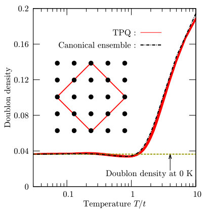 Figure 1
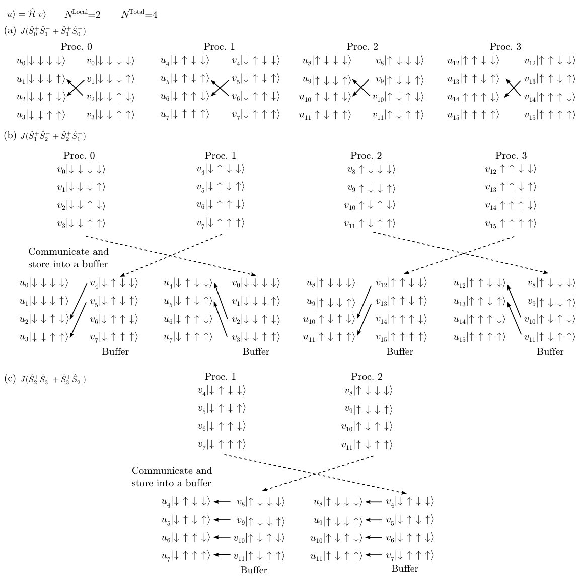 Figure 2
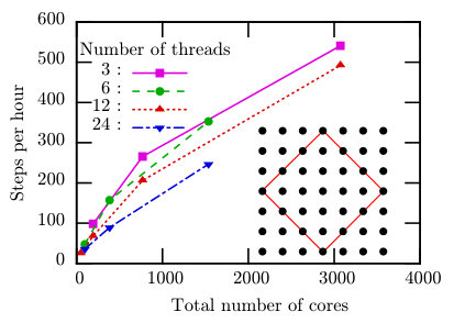 Figure 3
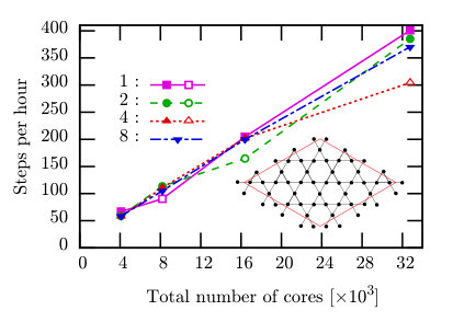 Figure 4
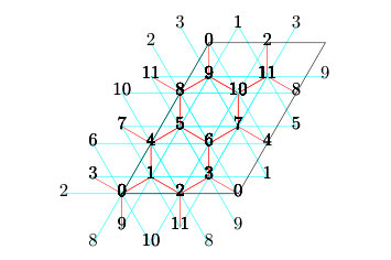 Figure 5
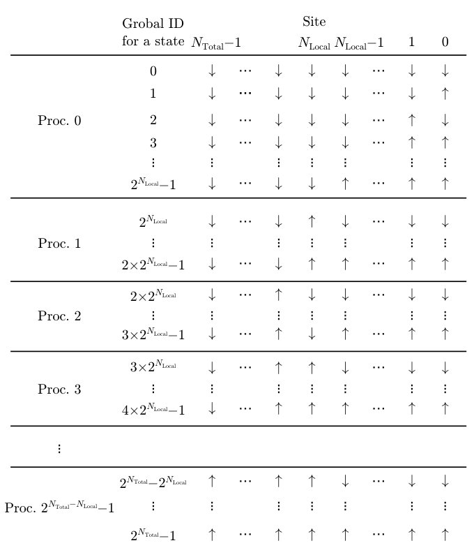 Figure 6
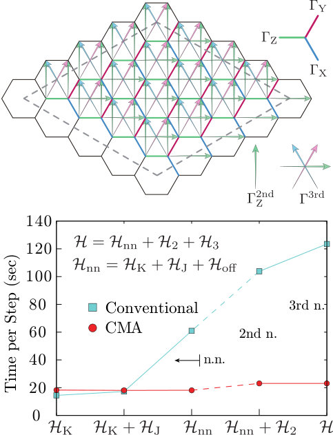 Figure 7
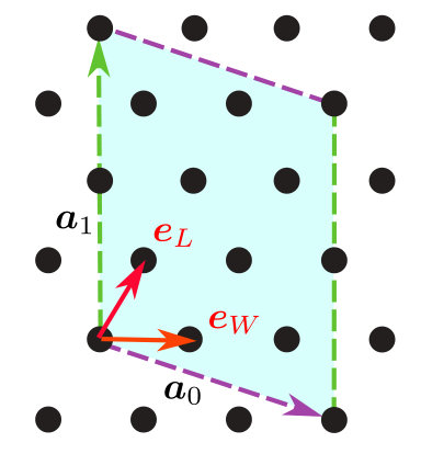 Figure 8
| Sekirei | K computer | |
| CPU | Xeon E5-2680v32 | SPARC 64™VIIIfx |
| Numer of cores per node | 24 | 8 |
| Peak performance | 960 GFlops | 128 GFlops |
| Main memory | 128 GB | 16 GB |
| Memory band width | 136.4 GB/s | 64 GB/s |
| Network topology | Enhanced hypercube | Six-dimensional mesh/torus |
| Network band width | 7 GB/s 2 | 5 GB/s 2 |
Peer Reviews
No public reviews on file for this paper yet. If you reviewed it on a platform where reviews are public (OpenReview, ICLR, NeurIPS, ICML), you can paste yours below so the community can read it here.
Code & Models
Videos
No videos yet. Explain this paper in a talk, walkthrough, or lecture? Add one.
Quantum Lattice Model Solver
Mitsuaki Kawamura
Kazuyoshi Yoshimi
Takahiro Misawa
Youhei Yamaji
Synge Todo
Naoki Kawashima
The Institute for Solid State Physics, The University of Tokyo, Kashiwa-shi, Chiba, 277-8581,Japan
Quantum-Phase Electronics Center (QPEC), The University of Tokyo, Bunkyo-ku, Tokyo, 113-8656, Japan
Department of Applied Physics, The University of Tokyo, Bunkyo-ku, Tokyo, 113-8656, Japan
JST, PRESTO, Hongo, Bunkyo-ku, Tokyo, 113-8656, Japan
Department of Physics, The University of Tokyo, Bunkyo-ku, Tokyo, 113-0033, Japan
Abstract
[aitch-phi] is a program package based on the Lanczos-type eigenvalue solution applicable to a broad range of quantum lattice models, i.e., arbitrary quantum lattice models with two-body interactions, including the Heisenberg model, the Kitaev model, the Hubbard model and the Kondo-lattice model. While it works well on PCs and PC-clusters, also runs efficiently on massively parallel computers, which considerably extends the tractable range of the system size. In addition, unlike most existing packages, supports finite-temperature calculations through the method of thermal pure quantum (TPQ) states. In this paper, we explain theoretical background and user-interface of . We also show the benchmark results of on supercomputers such as the K computer at RIKEN Advanced Institute for Computational Science (AICS) and SGI ICE XA (Sekirei) at the Institute for the Solid State Physics (ISSP).
keywords:
02.60.Dc Numerical linear algebra, 71.10.Fd Lattice fermion models, 75.10.Kt Quantum spin liquids
††journal: Computer Physics Communications
PROGRAM SUMMARY
Manuscript Title: Quantum Lattice Model Solver
Authors: Mitsuaki Kawamura, Kazuyoshi Yoshimi, Takahiro Misawa, Youhei Yamaji, Synge Todo, Naoki Kawashima
Program Title:
Journal Reference:
Catalogue identifier:
Program summary URL:
http://ma.cms-initiative.jp/en/application-list/hphi
Licensing provisions: GNU General Public License, version 3 or later
Programming language: C
Computer: Any architecture with suitable compilers including PCs and clusters.
Operating system: Unix, Linux, OS X.
RAM: Problem dependent. For example, less than one GB for a few-site system, and 3.8 TB for the 36-site Heisenberg model computed in this study.
Number of processors used: Problem dependent. We use up to 4,096 processors (32,768 cores) in this study.
Keywords: 02.60.Dc Numerical linear algebra, 71.10.Fd Lattice fermion models, 75.10.Kt Quantum spin liquids
Classification: 4.8 Linear Equations and Matrices, 7.3 Electronic Structure
External routines/libraries: MPI, BLAS, LAPACK
*Nature of problem:
*Physical properties (such as the magnetic moment, the specific heat, the spin susceptibility) of strongly correlated electrons at zero- and finite temperature.
*Solution method:
*Application software based on the full diagonalization method, the exact diagonalization using the Lanczos method, and the microcanonical thermal pure quantum state for quantum lattice model such as the Hubbard model, the Heisenberg model and the Kondo model.
*Restrictions:
*System size less than about 20 sites for a itinerant electronic system and 40 site for a local spin system.
*Unusual features:
*Finite-temperature calculation of the strongly correlated electronic system based on the iterative scheme to construct the thermal pure quantum state. This method is efficient for highly frustrated system which is difficult to treat with other methods such as the unbiased quantum Monte Carlo.
*Running time:
*Problem dependent. For example, when we compute the Heisenberg model on the kagome lattice without conservation, we can perform 400 iterations per hour.
1 Introduction
Comparison between experimental observation and theoretical analysis is a crucial step in condensed matter physics researches. Temperature dependence of the specific heat and the magnetic susceptibility, for example, has been studied to extract nature of low energy excitations and magnetic interactions among electrons, respectively, through comparison with the Landau’s Fermi liquid theory [1] and Curie-Weiss law [2].
For flexible and quantitative comparison with experimental data, an exact diagonalization approach [3], which can simulate quantum lattice models without any approximations is one of the most reliable numerical tools. Most numerical methods for general quantum lattice problems, which is not accompanied by the negative sign difficulty, are not exact and reliable error estimate for them is difficult. This drawback is serious especially when one wants to compare the results with experiments. Therefore, exact methods are valuable though they are usually available only for small size problems. They are important in two ways; as a tool for obtaining reliable answers to the original problem (when the original problem is a small size problem) and as a generator of reference data with which one can compare the results of other numerical methods (when the original problem is beyond the applicable range of the exact methods).
For the last few decades, the numerical diagonalization package for quantum spin Hamiltonians, TITPACK [4] has been widely used in the condensed matter physics community. Based on TITPACK, other numerical diagonalization packages such as KOBEPACK [5] and SPINPACK [6] have also been developed. There is another program performing such a calculation in the ALPS project (Algorithms and Libraries for Physics Simulations) [7]. However, the size of the target system is limited for TITPACK, KOBEPACK, and ALPS because they do not support the distributed memory parallelization. Although SPINPACK supports such parallelization and an efficient algorithm with the help of symmetries, this program package cannot handle the general interactions such as the Dzyaloshinskii-Moriya and the Kitaev interactions that recently receive extensive attention.
In addition, advances in quantum statistical mechanics [8, 9, 10, 11] open a new avenue for exact methods to finite-temperature calculations without the ensemble average. This development enables us to calculate finite-temperature properties of quantum many-body systems with computational costs similar to calculations of ground state properties. Now, it is possible to quantitatively compare theoretical predictions for temperature dependence of, for example, the specific heat and the magnetic susceptibility with experimental results [12]. However, the above program packages have not support this calculation yet. To perform the large-scale calculations directly relevant to experiments by utilizing the parallel computing architectures with small bandwidth and distributed memory, a user-friendly, multifunctional, and parallelized diagonalization package is highly desirable.
[aitch-phi], a flexible diagonalization package for solving a wide range of quantum lattice models, has been developed to overcome the problems in the previous program packages. In , we implement the Lanczos method for calculating the ground state and properties of a few excited states, thermal pure quantum (TPQ) states [11] for finite-temperature calculations, and full diagonalization method for checking results of Lanczos and TPQ methods at small clusters, with an easy-to-use and flexible user interface. By using , one can analyze a wide range of quantum lattice models including conventional Hubbard and Heisenberg models, multi-band extensions of the Hubbard model, exchange couplings that break SU(2) symmetry of quantum spins such as the Dzyaloshinskii-Moriya and the Kitaev interactions, and the Kondo lattice models describing itinerant electrons coupled to quantum spins. It is easy to calculate a variety of physical quantities such as the internal energy, specific heat, magnetization, charge and spin structure factors, and arbitrary one-body and two-body static Green’s functions at zero temperature or finite temperatures.
As we mention above, one of the aims of developing is to make a flexible diagonalization program package that enables us to directly compare the theoretical calculations and experimental data. In addition to the simple model Hamiltonians introduced in textbooks of quantum statistical physics, more complicated Hamiltonians inevitably appear to quantitatively describe electronic properties of real compounds. In the Lanczos and the TPQ simulation of the quantum lattice model in the condensed matter physics, the most time-consuming part is the multiplication of the Hamiltonian to a wavefunction. Excepting the case for the very small system, it is unrealistic to store all non-zero elements of the Hamiltonian in memory. Therefore we perform the multiplication by constructing the matrix elements of the Hamiltonian on the fly. To carry out the Lanczos and TPQ calculations efficiently, we implement two algorithms for massively parallel computation; one is the conventional parallelization based on the butterfly-structured communication pattern [13] (the butterfly method) and the other is newly developed method [the continuous-memory-access (CMA) method]. Because the numerical cost of the butterfly method is proportional to the number of terms in the second quantized Hamiltonian, it requires very long time to simulate the complicated Hamiltonian relevant to the real compounds. In contrast to the conventional algorithm, the newly developed method can realize the continuous memory access and numerical cost which does not depend on the number of terms during multiplication between the Hamiltonians and a wavefunction. In this paper, we also explain these two algorithms and compare their computational speed.
This paper is organized as follows: In Sec. 2, we introduce the basic usage of . How to download and build are explained in Sec. 2.1, and how to use is explained in Sec. 2.2. We also explain what types of models can be treated by using in Sec. 2.3. In Sec. 3, we detail algorithms implemented in . The representation of the Hilbert space adopted in is explained in Sec. 3.1. How to implement multiplication of the Hamiltonian to a wavefunction is explained in Sec. 3.2. Implementation of full diagonalization method, the Lanczos method, and the TPQ method is explained in Sec. 3.3, Sec. 3.4., Sec. 3.5, respectively. In Sec. 4, we explain the parallelization of multiplication of the Hamiltonian to a wavefunction. How to distribute the wavefunction for each process is explained in Sec. 4.1. In Sec. 4.2, we explain the conventional butterfly algorithm for parallelizing the Hamiltonian-wavefunction multiplication. We also explain another parallelization method (the CMA method), which is suitable for treating complicated quantum lattices models. In Sec. 5, we show the benchmark results of . In Sec. 5.1, we examine the validity of the TPQ method by using . In Sec. 5.2, we show the benchmark results of parallelization efficiency for 18-site Hubbard model and 36-site Heisenberg model on supercomputers. We also show the benchmark results of the CMA method in Sec. 5.3. Finally, Sec. 6 is devoted to the summary.
2 Basic usage of
2.1 How to download and build
The gzipped tar file, which contains the source codes, samples, and manuals, can be downloaded from the download site [14]. For building , a C compiler and the BLAS/LAPACK library[15] are prerequisite. To enable the parallel computations, the Message Passing Interface (MPI) library [16] is also required.
For building , the CMake utility [17] can be used as follows:
HOME/build/hphi PathTohphi $ make
Here, one builds in PathTohphi, is set to the path to the source tree path of (the top directory of ). If the CMake utility can not find the MPI library on the system, the executable is automatically compiled without the MPI library. In this example, CMake will choose a C compiler automatically. Instead, one can specify the compiler explicitly as follows:
Config make
where $Config is chosen from the following configurations:
gcc : GCC
- 2.
intel : Intel compiler + MKL library
- 3.
sekirei : Intel compiler + MKL library on ISSP system-B (Sekirei)
- 4.
fujitsu : Fujitsu compiler + SSL2 library on ISSP system-C (Maki)
For a system which does not have the CMake utility, we provide another way to generate Makefile’s using HPhiconfig.sh shell script. One can run HPhiconfig.sh in the top directory as follows:
make HPhi
Once the compilation finishes successfully, one can find the executable, HPhi, in src/ subdirectory.
2.2 How to use
Here, we briefly explain how to use . has two modes; Standard mode and Expert mode. The difference between them is the format of input files. For Expert mode, one has to prepare the files in the four categories below.
(1) Parameter files for specifying the model: In these files, one specifies the transfer integrals, interactions, and types of electronic state (local spins or itinerant electrons).
(2) Parameter files for specifying the calculation condition: In these files, one specifies the calculation methods (full diagonalization, Lanczos method, and TPQ method), the target of models (Spin, Kondo, and Hubbard models), number of sites and electrons, and the convergence criteria.
(3) Parameter files for correlation functions: By using these input files, one specifies one-body and two-body equal-time Green’s functions to be calculated.
(4) File for list of above input files: In this file, one should list the names of all the files that are necessary in the calculations.
For typical models in the condensed matter physics, such as the Heisenberg model and the Hubbard model, one can use in Standard mode. In Standard mode, one can specify all the input parameters by a single file with a few lines, from which the files described above are generated automatically before starting the calculation. It is thus much more easier to simulate and analyze these models in Standard mode as long as the model and the lattice is supported in Standard mode. The models supported in Standard mode will be explained in the following sections.
2.2.1 Flow of calculations
A typical flow of calculations in is shown as follows:
Make input files
An example of input file is shown for Standard mode below:
L = 4 W = 4 model = "Spin" method = "Lanczos" lattice = "square lattice" J = 1.0 2Sz = 0
Here L and W are a linear extents of square lattice, in and directions, respectively. Spin means the Heisenberg model, and J is the exchange coupling. By using this input file, one can obtain the ground state of the Heisenberg model for sites by performing the Lanczos method. Details of keywords in the input files can be found in the manuals [14].
In Expert mode, it is necessary to prepare all the files that specify the method, model parameters, and other input parameters. All the names of input files are listed in namelist.def. Details of the input files are also found in the manuals [14]. 2. 2.
Run
After preparing the input files, run a executable HPhi in terminal by setting option “-s” (or “--standard”) for Standard mode and “-e” for Expert mode as follows:
- (a)
Standard mode
$ ./HPhi -s StdFace.def
- (b)
Expert mode
$ ./HPhi -e namelist.def 3. 3.
Log and results
Log files and calculation results are output in the output directory which is automatically generated in the working directory. For the Lanczos and the full diagonalization methods, calculates and outputs the energy, the one-body Green’s functions, and the two-body Green’s functions from obtained eigenvectors. For the TPQ method, the inverse temperature, the energy and its variance are also obtained at each TPQ step. The specified one-body and two-body Green’s functions are output at specified interval.
2.3 Models
Here, we explain what types of models can be treated in . In Expert mode, the target models can be generally defined by the following Hamiltonian,
[TABLE]
where is a generalized transfer integral between site with spin and site with spin and is the generalized two-body interaction which annihilates a spin particle at site and a spin particle at site , and creates a spin particle at site and a spin particle at site . Here, () is the creation (annihilation) operator of an electron on site with spin or . For the Hubbard and Kondo models, the 1/2-spin fermions are only allowed. Note here that any system of localized spins can be regarded as a special case of the above Hamiltonian. Therefore, one can use for solving such quantum spin models by straight-forward interpretation of the spin interaction in terms of and in the above expressions. also has a capability of handling spins higher than .
In Standard mode, can treat the following models. (The titles of the following items are the corresponding keys for the model parameter in a Standard input file. Here, the keys, "Fermion HubbardGC", "SpinGC" and "KondoGC" are the grand-canonical version of "Fermion Hubbard", "Spin" and "Kondo", respectively.)
i) "Fermion Hubbard"/ "Fermion HubbardGC"
The Hamiltonian is given by
[TABLE]
where is the chemical potential, is the transfer integral between site and site , is the on-site Coulomb interaction, is the long-range Coulomb interaction between and sites. is the number operator at site with spin and .
ii) "Spin"/ "SpinGC"
The Hamiltonian is given by
[TABLE]
where is the longitudinal magnetic field, is the transverse magnetic field, and is the single-site anisotropy parameter. is the coupling constant between the component of spins at site and site , and is the coupling constant between the component of the spin at site and the component of the spin at site , where . is the -axis spin operator at site .
iii) "Kondo"/ "KondoGC"
The Hamiltonian is given by
[TABLE]
where , , , and are the same as those in the “Fermion Hubbard”. is the coupling constant between spins of an itinerant electron and a localized one.
2.4 Lattice
Here, we explain available lattice structures in . In Expert mode, arbitrary lattice structures can be treated by specifying connections of sites. In contrast to Expert mode, one can easily specify the conventional lattice structures by using Standard mode. Standard mode supports the chain lattice, the ladder lattice, the square lattice (examples are shown in insets of Figs. 5 and 6), the triangular lattice (Fig. 1), the honeycomb lattice (Fig. 2), and the kagome lattice (an example of kagome lattice is shown inset of Fig. 7). In Standard mode, one can construct the above two-dimensional lattices by specifying four integer parameters, a0W, a0L, a1W, and a1L and two unit lattice vectors and . By using these parameters and unit vectors, a superlattice spanned by and is specified. We show an example of triangular lattice in Fig. 1.
2.5 Samples
There are some sample input files and reference results in samples/ directory. For example, samples/Standard/Hubbard/square/ is the directory containing files for the computation of the Hubbard model on the -site square lattice. We can perform the calculation of the ground state by running as Standard mode as follows:,
$ ./HPhi -s StdFace.def
While running, dumps information to the standard output. We can check the geometry of the calculated system by using lattice.gp which is generated by ; it is read by gnuplot [18] as follows:
$ gnuplot lattice.gp
Then, gnuplot displays the shape of the system and indices of sites (See Fig. 2 as an example. This figure is obtained by using samples/Standard/Spin/Kitaev/StdFace.def).
The calculated results are written in output/. In output/zvo_energy.dat the total energy, the number of doublons (sites occupied by two electrons with opposite spins), and the magnetization along the axis are output. We can compare it with the reference data in output_Lanczos/zvo_energy.dat below samples/Standard/Spin/Kitaev/. Correlation functions are obtained in output/zvo_cisajs.dat and output/zvo_cisajscktalt.dat.
When executed in Standard mode, creates various input files, such as calcmod.def and modpara.def, that can be used in Expert mode. Editing those files may be the easiest way of using for models not supported in Standard mode. To do so, after making all the necessary modifications, run by the following command:
$ ./HPhi -e namelist.def
By using Expert mode, one can perform more flexible calculations.
3 Algorithms implemented in
In , we implement the following three methods; full diagonalization, exact diagonalization by the Lanczos method for ground state calculation, the TPQ method for calculation of physical properties at finite temperatures. In this section, we first explain the internal representation of the Hilbert space in and how to implement the multiplication of the Hamiltonian to a wavefunction in . Next, we explain above three methods.
3.1 Internal representation of Hilbert space in
To specify a state of a site in , we use an -ary, which takes one of different values. For example, in the case of an itinerant electronic system, the local site may take four states, , and , and therefore it is natural to represent it by a 4-ary. In this representation, a basis is labeled by as . Here, represents the -digit -ary number, i.e.,
[TABLE]
To use the standard bitwise operations (e.g. logical disjunction and exclusive or), we decompose the 4-ary representations as the following example: A basis of the 4-site system is indexed by a quartet of -digit binary numbers as
[TABLE]
For the Kondo system, the local sites are classified into itinerant electron part and localized spin part. However, for simplicity, we use 4-ary representations likewise for the itinerant electronic system, i.e., we represent a localized spin by or .
For localized spin- systems (), to represent Hilbert spaces we use -ary representation. For example, in a spin-1 system the wavefunction is represented as . To treat the spin- system, we used Bogoliubov representation shown in A.1. In , we can treat the more complicated spin systems such as the spin angular momentums have different values at each site (mixed spin systems).
In general, at -th site with the spin angular momentum , the Hilbert space at -th site is represented by -ary number and the Hilbert space of the system is represented by where and is the whole number of sites. By using the multiplications of the -ary number, we represent the mixed spin systems as follows:
[TABLE]
We note that, when the canonical system is selected by the input file, automatically constructs the restricted Hilbert space that has the specified particle number or total . To perform the efficient reverse lookup in the restricted Hilbert space, we use the two-dimensional search method [4, 19]. We also use the algorithm quoted in [20] as “finding the next higher number after a given number that has the same number of 1-bits” to perform an efficient two-dimensional search method.
3.2 Full Diagonalization method
We generate the matrix of by using above-mentioned basis set (, is the dimension of the Hilbert space): . By diagonalizing this matrix, we can obtain all the eigenvalues and normalized eigenvectors (). In the diagonalization, we use lapack routine such as dsyev or zheev. We also calculate and output the expectation values . These values are used for the finite-temperature calculations.
From , we calculate finite-temperature properties by using the ensemble average
[TABLE]
In the actual calculation, the ensemble averages are performed as a postprocess.
3.3 Multiplying Hamiltonian to wavefunctions (matrix-vector product)
Here, we explain the main operation in , multiplying the Hamiltonian to the wavefunctions. Because the dimension of the wavefunction becomes exponentially large by increasing the number of sites, it is impossible to store the whole matrix in the actual calculations. Thus, in the Lanczos (Sec. 3.4) and the TPQ (Sec. 3.5) methods, we only store the wavefunctions and calculate the matrix elements at each interaction on the fly.
We explain the procedure of multiplying the Hamiltonian to the wavefunctions by taking the 4-site Heisenberg model with on the chain with periodic boundary condition as an example. The Hamiltonian is block-diagonalized with blocks being characterized by the total magnetization, . For the block satisfying , the wavefunction can be represented by using the simultaneous eigenvectors of all ’s as
[TABLE]
Here, the quartet of up or down arrows, which we call a “configuration” in what follows, specifies a basis vector. In the actual calculations, we store the list of the configurations.
The Hamiltonian is defined as
[TABLE]
where and are defined as follows,
[TABLE]
To reduce the numerical cost, we store diagonal elements such as for each configuration. In contrast to the diagonal terms, changes the configuration, e.g. ,
[TABLE]
In , if the exchange operation is possible, the operation is performed by bit operations as follows:
[TABLE]
where ^ represents the “bitwise exclusive or”. Before performing the exchange operator, we count bits in the configuration and judge whether the exchange operation is possible or not. If the exchange operation is not possible, we do not perform the operation and regard the contribution from the configuration as zero, i.e. ,
[TABLE]
We note that the sign arises from the exchange relation between fermion operators in the itinerant electrons systems such as Hubbard models, while the sign does not appear in the localized spin systems. To obtain the sign, it is necessary to count the parity of the given bit sequences. We use the algorithm for parity counting that is explained in the literature [20].
3.4 Lanczos method
For the sake of completeness, we briefly review the principle of the Lanczos method. For more details see, for example, the TITPACK manual [2] and the textbook by M. Sugihara and K. Murota [21].
The Lanczos method is based on the power method. In the power method, by successive operations of the Hamiltonian to the arbitrary vector , we generate bases . The obtained linear space is called the Krylov subspace. The initial vector is represented by the superposition of the eigenvectors (corresponding eigenvalues are ) of as
[TABLE]
We note that all the eigenvalues are real number because Hamiltonian is a Hermitian operator. By operating to the initial vector, we obtain the relation as
[TABLE]
where we assume that has the maximum absolute value of the eigenvalues. This relation shows that the eigenvector of becomes dominant for sufficiently large . We note that the Krylov subspace does not change under the constant shift of the Hamiltonian [22], i.e.,
[TABLE]
where is the identity matrix and is a constant. By taking constant as the large positive value, the leading part of becomes the maximum eigenvectors and vice versa. Thus, by constructing the Krylov subspace, we can obtain eigenvalues around both the maximum and the minimum eigenvalues.
In the Lanczos method, we successively generate the normalized orthogonal basis from the Krylov subspace . We define the initial vector and associated components as , . From this initial condition, we can obtain the normalized orthogonal basis as follows:
[TABLE]
From these definitions, it is obvious that and are real number.
In the subspace spanned by these normalized orthogonal basis, the Hamiltonian is transformed as
[TABLE]
Here, is the matrix whose column vectors are . We note that ( is an identity matrix). is a tridiagonal matrix and its diagonal elements are and subdiagonal elements are . It is known that the eigenvalues of are well approximated by the eigenvalues of for sufficiently large . The original eigenvectors of is obtained by , where are the eigenvectors of . From , we can obtain the eigenvectors of . However, in the actual calculations, it is difficult to keep because its dimension is too large to store [dimension of = (dimension of the total Hilbert space) (number of Lanczos iterations)]. Thus, to obtain the eigenvectors, in the first Lanczos calculation, we keep because its dimension is small (upper bound of the dimensions of is the number of Lanczos iterations). Then, we again perform the same Lanczos calculations after we obtain the eigenvalues from the Lanczos methods. From this procedure, we obtain the eigenvectors from .
In the Lanczos method, by successive operations of the Hamiltonian on the initial vector, we obtain accurate eigenvalues around the maximum and minimum eigenvalues and associated eigenvectors by using only two vectors whose dimensions are the dimension of the total Hilbert space. In , to reduce the numerical cost, we store two additional vectors; a vector for accumulating the diagonal elements of the Hamiltonian, and another vector for the list of the restricted Hilbert space explained in Sec. 3.3. The dimension of these vectors is that of the Hilbert space. As detailed below, to obtain the eigenvector by the Lanczos method, one additional vector is necessary. Within some number of iterations, we obtain accurate eigenvalues near the maximum and minimum eigenvalues. The necessary number of iterations is small enough compared to the dimensions of the total Hilbert space. We note that it is shown that the errors of the maximum and minimum eigenvalues become exponentially small as a function of Lanczos iterations (for details, see Ref. [21]). Details of generating the initial vectors and convergence conditions are shown in A.2 and A.3, respectively.
3.4.1 Inverse iteration method
In some cases, the accuracy of obtained eigenvectors by the Lanczos method is not enough for calculating the correlation functions. To improve the accuracy of the eigenvectors, we implement the inverse iteration method in , which is also implemented in TITPACK [4].
By using the approximate value of the eigenvalues , by successively operating to the initial vector , we can obtain the accurate eigenvector for . The linear simultaneous equation for such procedure is given by
[TABLE]
By solving this equation by using the conjugate gradient (CG) method, we can obtain the eigenvector. We note that we take as the eigenvector obtained by the Lanczos method and add small positive number to for stabilizing the CG method. Although we can obtain more accurate eigenvector by using this method, additional four vectors are necessary to perform the CG method.
3.5 Finite-temperature calculations by TPQ method
The method of the TPQ states is based on the fact [10] that it is possible to calculate the finite-temperature properties from a few wavefunctions (in the thermodynamic limit, only one wavefunction is necessary) without the ensemble average. In what follows we describe the prescription proposed in [11], which we adopt in . Such wavefunctions that replace the ensemble average are called TPQ states. Because a TPQ state can be generated by operating the Hamiltonian to the random initial wavefunction, we directly use the routine of the Lanczos method to the TPQ calculations. Here, we explain how to construct the TPQ state, which offers a simple way for finite-temperature calculations.
Let be a random initial vector. How to generate is described in A.4. By operating ( is a constant, represents the number of sites) to , we obtain the -th TPQ states as
[TABLE]
From , we estimate the corresponding inverse temperature as
[TABLE]
where is the internal energy. Arbitrary local physical properties at are also estimated as
[TABLE]
In a finite-size system, a finite statistical fluctuation is caused by the choice of the initial random vector. To estimate the average value and the error of the physical properties, we perform some independent calculations by changing . Usually, we regard the standard deviations of the physical properties as the error bars.
4 Parallelization
4.1 Distribution of wavefunction
In the calculation of the exact diagonalization based on the Lanczos method or the finite-temperature calculations based on the TPQ state, we have to store the many-body wavefunction on the random access memory (RAM). This wavefunction becomes exponentially large with increasing the number of sites. For example, when we compute the 40-site spin system in the unconserved condition, its dimension is and its size in RAM becomes about 17.6 TB (double precision complex number). Such a large wavefunction can be treated by distributing it to many processes by utilizing distributed memory parallelization.
In , the ranks of the processes are labeled by using the leftmost bits in the bit representation of the wavefunction basis. When the leftmost bits corresponding to a -site subsystem are chosen to label the ranks of the processes, the number of processes have to be (for spin systems) or (for itinerant electron systems). Then, each process keeps partial wavefunction of the complementary -site subsystem. Distribution of wavefunctions of an spin-1/2 system is illustrated in Fig. 3. We note that the configuration of the sites is fixed in the same process.
For example, we show the distribution of the wavefunction of the -site spin system in the unconserved condition in Fig. 3 (the number of processes is ). Each process has the wavefunction having components and we can obtain the wavefunction of the entire system by connecting local wavefunctions of all processes.
4.2 Parallelization of Hamiltonian-vector product
The most time-consuming procedure in a calculation of the Lanczos method or the TPQ state is the multiplication of the Hamiltonian with a vector (), where and are wavefunctions distributed to all the processes. We parallelize this procedure with the aid of Message Passing Interface (MPI) [16].
Here, we explain the parallelization procedure by taking a spin exchange term as an example. Because the spin exchange occurs between two sites, we use one of the following three procedures according to the type of the two sites (See Fig. 4). When the numbers specifying the both sites are smaller than , we can perform this exchange independently in each process; there is no inter-process communication [Fig. 4(a)]. If one of two sites has an index equal to or larger than , first the local wavefunction is communicated between two processes connected with the exchange operator and stored in a buffer. Then we compute the remaining exchange operator [Fig. 4(b)]. We employ this procedure also when both sites are equal to or larger than [Fig. 4(c)]. In this case, some processes do not participate the calculation; it causes a load imbalance. However, it is not so serious problem; the computational time of this case is shorter than those time of the previous two cases because the arrays are accessed sequentially in this case.
4.3 Continuous-memory-access (CMA) method
Numerical costs become smaller if all operations can be done similar to Fig. 4(a) in which the memory access is limited within each process. In addition, if we can apply simultaneously the all terms in the second quantized Hamiltonian acting to the part of wavefunctions continuously stored in the CPU-cache memory, the numerical cost becomes small and independent from the number of the terms. Indeed, we can partially convert the conventional algorithm into an efficient algorithm by employing a permutation of the bits. By the permutation, we can also achieve continuous memory access, which is usually faster than random access happening inevitably in the conventional algorithm (Sec. 4.2). In this section, we explain the newly developed algorithm to realize the continuous memory access and to enhance the computing efficiency.
Any partial Hamiltonians acting on the rightmost bits are represented by a by matrix that acts on successive components, namely, [math] th to -th components, of the wavefunction. Then, if the () rightmost bits are permuted in the bit representation of the basis as,
[TABLE]
where (), the partial Hamiltonians acting on the th bit, th bit, and so on, are again represented by a matrix that acts on the successive components of the wavefunction. If we find an integer that satisfies and decompose the total Hamiltonian into the partial Hamiltonians that act on sets of successive bits that overlap each other, the multiplication of the Hamiltonian is implemented with continuous memory access by repeating the -bits permutation.
When the wavefunctions are distributed in many processes, the -bits permutation is achieved by the following steps. First, we permute the components in the wavefunction within the rank process, (), with a buffer as
[TABLE]
Then, we call an MPI all-to-all routine to transfer the components in the buffer to another buffer in other processes as
[TABLE]
Finally, the following permutation of the components of the wavefunctions completes the -bit permutation of the distributed wavefunction:
[TABLE]
Details of the continuous access will be reported elsewhere [23]. The CMA method is implemented in Standard mode for spins without total conservation in the present version of 111 Since the implementation of the CMA method is more complicated than that of the conventional algorithm explained in the previous section (Sec. 4.2), the algorithm has not been implemented for other systems yet. .
5 Benchmark results and performance
In this section, we show benchmark results of . First, we examine the accuracy of the finite-temperature calculations based on the TPQ algorithm [11] by comparing the results with the exact ensemble averages calculated by the full diagonalization. For small system sizes, we can easily perform the same calculation on our own PCs. Second, we show the parallelization efficiency of for large system sizes on supercomputers. We have carried out TPQ simulations of two typical models, namely, an 18-site Hubbard model on a square lattice and a 36-site Heisenberg model on a kagome lattice, with changing numbers of threads and CPU cores, where the number of CPU cores equals the number of threads times the number of MPI processes. We also show performance of the CMA method.
5.1 Benchmark results of TPQ simulations
To examine the validity of the TPQ calculation, we compute the temperature dependence of the doublon density of the Hubbard model () for an 8-site cluster with the periodic boundary condition. The shape of the cluster is illustrated in the inset of Fig. 5. The Hubbard model is defined by setting , , for the nearest-neighbor pairs of sites, , and for further neighbor pairs of sites. An example of the input file for the 8-site Hubbard model used in this calculation is shown as follows:
a0W = 2 a0L = 2 a1W = -2 a1L = 2 model = "Fermion Hubbard" method = "TPQ" lattice = "square lattice" t = 1.0 U = 8.0
In Fig. 5, we show the temperature dependence of the doublon density, , calculated by the TPQ state and by the canonical ensemble. We confirm that the TPQ calculations well reproduce the results of the canonical ensemble average. In addition to the finite-temperature calculations, we perform the ground state calculations by the Lanczos method and the calculated doublon density at zero temperature is plotted by the dashed line. We also confirm that doublon density at low temperature well converges to the value of the ground state. All the results show the validity of the TPQ method.
5.2 Parallelization Efficiency
Here, we carry out TPQ simulations for large system sizes with changing numbers of threads and processes to examine parallelization efficiency of . We choose two typical models; a half-filled 18-site Hubbard model on a square lattice and a 36-site Heisenberg model on a kagome lattice. The speedup of the simulation for the 18-site Hubbard model with up to 3,072 cores is measured on SGI ICE XA (Sekirei) at ISSP (Table 1). The speedup of the large-scale simulation for the 36-site Heisenberg model with up to 32,768 cores is examined by using the K computer at RIKEN AICS (Table 1).
5.2.1 18-site Hubbard model
We perform the TPQ simulations for the half-filled 18-site Hubbard model on the square lattice illustrated in the inset of Fig. 6. Here, we employ the subspace of the Hilbert space that satisfies . Then, the dimension of the subspace is , where represents the binomial coefficient. The input file used in this calculations is shown below:
a0W = 3 a0L = 3 a1W = -3 a1L = 3 model = "Fermion Hubbard" method = "TPQ" lattice = "square lattice" t = 1.0 U = 8.0 nelec = 18 2Sz = 0
In Fig. 6, we can see significant acceleration caused by the increase of CPU cores. This acceleration is almost linear up to 192 cores, and is weakened as we further increase the number of cores. This weakening of the acceleration comes from the load imbalance in the conserved simulation. For example, when we use 3 OpenMP threads and 1024 MPI processes, the number of sites associated with the ranks of processes ( in Sec. 4.1 ) becomes 5, and the number of sites in the subsystem in each process ( in Sec. 4.1) becomes 13. Each process has different numbers of up- and down- spin electrons. In the process which has the largest Hilbert space, there are six up-spin electrons and six down-spin electrons, and the Hilbert space becomes . On the other hand, the process which has the smallest Hilbert space has nine up-spin electrons, nine down-spin electrons and the dimensional Hilbert space. This large difference of the Hilbert-space dimension between each process causes a load imbalance. This effect becomes large as we increase the number of processes.
When we fix the total number of cores (for examples 1536 cores), we can find that the process-major computation (256 processes with 6 threads) is faster than the thread-major computation (64 processes with 24 threads). Since the numerical performance of both of them are equivalent, this behavior seems strange at first sight. The origin of difference might be explained as follows: When we double the number of processes, the amount of data communicated by each process at once becomes a half of the original size, and the communication time decreases. On the other hand the communicated data-amount and the communication time is unchanged even if we double the number of threads. In other words, the algorithm described in Sec. 4.2 parallelizes calculation and also communication.
5.2.2 36-site Heisenberg model
We perform the TPQ calculations for the 36-site Heisenberg model on the kagome lattice with hybrid parallelization by using up to 32,768 cores. Here, we employ the -dimensional () Hilbert space without the conservation. Although the canonical ( conserved) calculation is faster than the grand-canonical ( unconserved) calculation, we sometimes employ the latter for the TPQ calculation. The finite-size effect is much smaller in the grand-canonical TPQ state than in the canonical TPQ state [26]. Figure 7 shows the speedup of this calculation on the K computer. In contrast to the canonical calculation in the previous section, we obtain the almost linear scaling even we use the very large number of cores (more than ten thousands cores). In the grand-canonical calculation, each process has a Hilbert space of the same size. Therefore, there is no load imbalance that appears prominently in the canonical calculation. Due to the high throughput of the inter-node data transfer on the K computer, the parallelization efficiency from 4,096 cores to 32,768 cores reaches 82% and change in number of MPI processes does not largely affect the speed. Except for some cases (open symbols in Fig. 7), in the group of the same number of cores (for example, 16384 cores), we can not find any significant difference between the performance of the thread-major computation (2048 processes with 8 threads) and that of the process-major computation (16384 processes with 1 thread). On the other hand when we calculate the same system by using 3,072 cores on Sekirei, the speed of the computation by using 128 processes with 24 threads and that speed by using 1024 processes with 3 threads become 29 steps / hour and 71 steps / hour, respectively; we can find the advantage of the process-major computation on Sekirei as in the previous section. It is thought that because the communication time on Sekirei is longer than that on the K computer, the parallelization of the communication by increasing the number of processes is more effective on Sekirei than on the K computer.
For some cases the speed becomes exceptionally slow (corresponding conditions are shown as open symbols). This slowdown occurs when the number of processes is 8,192, and it remains even if we change the lattice to the one-dimensional chain. We consider the reason of the slowdown as follows. There are three effects on the computational speed by increasing processes: first, the numerical cost per single process and the data size per single communication decrease in inversely proportional to the number of processes (positive effect), second, the frequency of communication increases (negative effect), and, finally, the load balancing becomes worse (negative effect). Therefore we consider the slowdown comes from the competition of these effects.
5.3 Benchmark of continuous-memory-access method
In this section, we show benchmark results of the continuous-memory-access parallelization algorithm, namely, the CMA method in , which is briefly explained in Sec. 4.3. The CMA method is particularly advantageous when the Hamiltonian does not possess the U(1) symmetry or the SU(2) symmetry that make the total charge and the total magnetization good quantum numbers. A typical example is the Kitaev model discussed below. For such Hamiltonians, we cannot use the canonical mode. Especially, the CMA method is much faster than the conventional parallelization scheme explained in Sec.4.2 when inter-site interactions are dense and complicated. This is because the cost for the computation and memory-transfer for the bit permutation does not depend on the number of terms or the complexity of the Hamiltonian as long as the range of interaction is not too long, while, in the conventional parallelization scheme, the cost for the Hamiltonian operations increases as it has more terms. To compare performance of the CMA method and the conventional parallelization scheme, here, we carried out TPQ simulations of a spin Hamiltonian with complicated spin-spin interactions.
We show the benchmark results of the TPQ simulation for a spin Hamiltonians of iridium oxide, Na2IrO3, which was derived by utilizing ab initio electronic band structures and many-body perturbation theory [12]. The Hamiltonian is defined on a honeycomb structure and has complicated inter-site spin-spin interactions that can be classified into five parts as follows:
[TABLE]
where the first term represents the Kitaev Hamiltonian [27], the second term describes diagonal exchange couplings between nearest-neighbor (n.n.) spins, and the third term describes complicated off-diagonal spin-spin interactions. The fourth term and the fifth term describe the second neighbor (2nd n.) interactions and the third neighbor (3rd n.) interactions, respectively. Details of the Hamiltonians are given in the previous study [12].
In the lower panel of Fig. 8, elapsed time per TPQ step for the conventional and the CMA method is shown for a Kitaev Hamiltonian, , a Kitaev-Heisenberg Hamiltonian, , a n.n. Hamiltonian, , a Hamiltonian including 2nd n. interactions, , and the ab initio Hamiltonian . Here, we use 16 nodes (24 cores per node) on Sekirei at ISSP the TPQ simulation with 3 threads and 128 processes. Even when the number of the coupling term increases, from the sparse Kitaev Hamiltonian to the dense and complicated Hamiltonian of Na2IrO3, , the elapsed time per TPQ step of the CMA method does not show significant increase while the elapsed time of the conventional scheme shows significant increase.
Although, for the sparse Kitaev Hamiltonian , the conventional scheme shows slightly better performance than that of the CMA method, the CMA method is three times faster than the conventional one even for the n.n. Hamiltonian . Furthermore, even though, from to , the number of the bonds clearly increases, the elapsed time per TPQ step of the CMA method only shows slight increase.
6 Summary
To summarize, we explain the basic usage of in Sec. 2. By preparing one file within ten lines, for typical models in the condensed matter physics, one can easily perform the exact diagonalization based on the Lanczos method or finite-temperature calculations based on the TPQ method. By using the same file, one can also perform the large-scale calculations on modern supercomputers. By properly editing the intermediate input files generated by Standard mode execution, it is also easy to perform the similar calculations for complicated Hamiltonians that describe the low-energy physics of real materials. This flexibility and user-friendly interface are the main advantage of and we expect that will be a useful tool for broad spectrum of scientists including experimentalists and computer scientists.
In Sec. 3, we explain the basic algorithms implemented in . Although the Lanczos method and the TPQ method are detailed in the literature, to make our paper self-contained, we explain the essence of these methods. Furthermore, in Sec. 4, we detail the parallelization methods of the multiplication of Hamiltonian to the wavefunctions; one is the conventional butterfly method and another one is the newly developed method. We also show the benchmark results of on supercomputers in Sec. 5. The results indicate that parallelization of works well on these supercomputers and the computational time is drastically reduced.
We also introduce the new algorithm for parallelization, i.e., the (CMA) method. The main advantage of this method is that the speed does not depend on the number of terms in the Hamiltonians, while the computational cost of the conventional butterfly method is proportional to the number of terms in the Hamiltonians. Thus, the CMA method is suitable for treating the complicated Hamiltonians for real materials. Actually, for the low-energy model of Na2IrO3, we show that the speed of the CMA method is about six times faster than that of the conventional method. So far, the CMA method is applicable to the limited class of Hamiltonians and lattice geometries. In addition, its efficiency largely depends on the models. It is a remaining challenge to remove the limitation from the CMA method.
Recent development of the theoretical tools for obtaining the low-energy models of real materials enable us directly compare the theoretical results and experimental results. Although the limitation of the system size is severe, the exact analyses based on the Lanczos method or the TPQ method offer a firm basis for examining the validity of the theoretical results. The present version of can calculate only the static physical quantities, which is difficult to be directly measured in experiments. Extending to calculate dynamical properties such as the dynamical spin/charge structure factors and the optical conductivity is a promising way to make more useful. Such an extension will be reported in the near future.
7 Acknowledgements
We would like to express our sincere gratitude to Prof. Hidetoshi Nishimori and Mr. Daisuke Tahara. Implementation of the Lanczos algorithm in written in C is based on the pioneering diagonalization package TITPACK ver. 2 written in Fortran by Prof. Nishimori. For developing the user interface of , we follow the design concept of the user interface in the program for variational Monte Carlo method developed by Mr. Tahara. A part of the user interface in is based on his original codes. We would also like to thank the support from “Project for advancement of software usability in materials science” by The Institute for Solid State Physics, The University of Tokyo, for development of ver.1.0. We thank the computational resources of the K computer provided by the RIKEN Advanced Institute for Computational Science through the General Trial Use project (hp160242). This work was also supported by Grant-in-Aid for Scientific Research (15K17702, 16H06345, and 16K17746) and Building of Consortia for the Development of Human Resources in Science and Technology from the MEXT of Japan and supported by PRESTO, JST. We also thank numerical resources from the Supercomputer Center of the Institute for Solid State Physics, The University of Tokyo.
Appendix A Details of implementation
A.1 Bogoliubov representation
In the spin system, the spin indices in input files of transfer, InterAll, and correlation functions are specified by using the Bogoliubov representation. Spin operators are written by using creation/annihilation operators as follows:
[TABLE]
A.2 Initial vector for the Lanczos method
In the Lanczos method, an initial vector is specified with initial_iv() defined in an input file for Standard mode or a ModPara file for Expert mode. A type of an initial vector can be selected from a real number or complex number by using InitialVecType in a ModPara file.
For canonical ensemble and initial_iv
A non-zero component of a target of Hilbert space is given by
[TABLE]
where is a total number of the Hilbert space and is added to avoid selecting the special configuration for a default value initial_iv . When a type of an initial vector is selected as a real number, a coefficient value is given by , while as a complex number, the value is given by .
- 2.
For grand canonical ensemble or initial_iv
An initial vector is given by using a random generator, i.e. coefficients of all components for the initial vector is given by random numbers. The seed is calculated as
[TABLE]
where is a number given by an input file (parameter initial_iv), is the thread ID, is the number of threads, and is the process ID. Therefore the initial vector depends both on initial_iv and the number of processes. Random numbers are generated by using SIMD-oriented Fast Mersenne Twister (dSFMT) [28].
A.3 Convergence condition for Lanczos method
In , we use dsyev (routine of lapack) for diagonalization of . We use the energy of the first excited state of as a criteria of convergence. In the standard setting, after five Lanczos step, we diagonalize every two Lanczos step. If the energy of the first excited states agrees with the previous energy within the required accuracy, the Lanczos iteration finishes. The accuracy of the convergence can be specified by LanczosEps (ModPara file in Expert mode).
After obtaining the eigenvalues, we again perform the Lanczos iteration to obtain the eigenvector. From the eigenvectors , we calculate energy and variance . If agrees with the eigenvalues obtained by the Lanczos iteration and is smaller than the specified value, we finish the diagonalization.
If the accuracy of Lanczos method is not enough, we perform the CG method to obtain the eigenvector. As an initial vector of the CG method, we use the eigenvectors obtained by the Lanczos method in the standard setting. This often accelerates the convergence.
A.4 Initial vector for the TPQ method
For TPQ method, an initial vector is given by using a random number generator, i.e. coefficients of all components for the initial vector are given by random numbers. The seed is calculated as
[TABLE]
where , , , and are the same as those for the Lanczos method [Eqn. (43)]. indicates the counter of trials, which is equal to or less than the total number of trials NumAve in an input file for Standard mode or a ModPara file for Expert mode. We can select a type of initial vector from a real number or complex number by using InitialVecType in a ModPara file. indicate the thread ID, the number of threads, the process ID, respectively; the initial vector depends both on initial_iv and the number of processes.
References
The reference list from the paper itself. Each links out to its DOI / PubMed record.
- 1[1] D. Pines, P. Nozières, The Theory of Quantum Liquids, Perseus Books Publishing, 1999.
- 2[2] C. Kittel, Introduction to solid state physics, John Wiley & Sons, Inc., 2005.
- 3[3] E. Dagotto, Rev. Mod. Phys. 66 (1994) 763–840.
- 4[4] http://www.stat.phys.titech.ac.jp/ nishimori/titpack 2_new/index-e.html.
- 5[5] http://quattro.phys.sci.kobe-u.ac.jp/Kobe_Pack/Kobe_Pack.html.
- 6[6] http://www-e.uni-magdeburg.de/jschulen/spin/.
- 7[7] B. Bauer, L. D. Carr, H. G. Evertz, A. Feiguin, J. Freire, S. Fuchs, L. Gamper, J. Gukelberger, E. Gull, S. Guertler, A. Hehn, R. Igarashi, S. V. Isakov, D. Koop, P. N. Ma, P. Mates, H. Matsuo, O. Parcollet, G. PawナPwski, J. D. Picon, L. Pollet, E. Santos, V. W. Scarola, U. Schollwテカck, C. Silva, B. Surer, S. Todo, S. Trebst, M. Troyer, M. L. Wall, P. Werner, S. Wessel, Journal of Statistical Mechanics: Theory and Experiment 2011 (05) (2011) P 05001. [link] . URL http://stacks.iop.o
- 8[8] M. Imada, M. Takahashi, J. Phy. Soc. Jpn. 55 (10) (1986) 3354–3361.
