Overcoming the Sign Problem at Finite Temperature: Quantum Tensor Network for the Orbital $e_g$ Model on an Infinite Square Lattice
Piotr Czarnik, Jacek Dziarmaga, and Andrzej M. Ole\'s

TL;DR
This paper demonstrates that tensor network methods can effectively overcome the quantum Monte Carlo sign problem at finite temperature for the orbital $e_g$ model, accurately capturing phase transition properties and critical exponents.
Contribution
It introduces a tensor network approach to study a sign-problematic 2D quantum model at finite temperature, providing precise estimates of critical temperature and exponents.
Findings
Confirmed finite order parameter below $T_c$
Estimated critical temperature $T_c$ accurately
Critical exponents within 1% of 2D Ising universality
Abstract
The variational tensor network renormalization approach to two-dimensional (2D) quantum systems at finite temperature is applied for the first time to a model suffering the notorious quantum Monte Carlo sign problem --- the orbital model with spatially highly anisotropic orbital interactions. Coarse-graining of the tensor network along the inverse temperature yields a numerically tractable 2D tensor network representing the Gibbs state. Its bond dimension --- limiting the amount of entanglement --- is a natural refinement parameter. Increasing we obtain a converged order parameter and its linear susceptibility close to the critical point. They confirm the existence of finite order parameter below the critical temperature , provide a numerically exact estimate of~, and give the critical exponents within of the 2D Ising universality class.
Click any figure to enlarge with its caption.
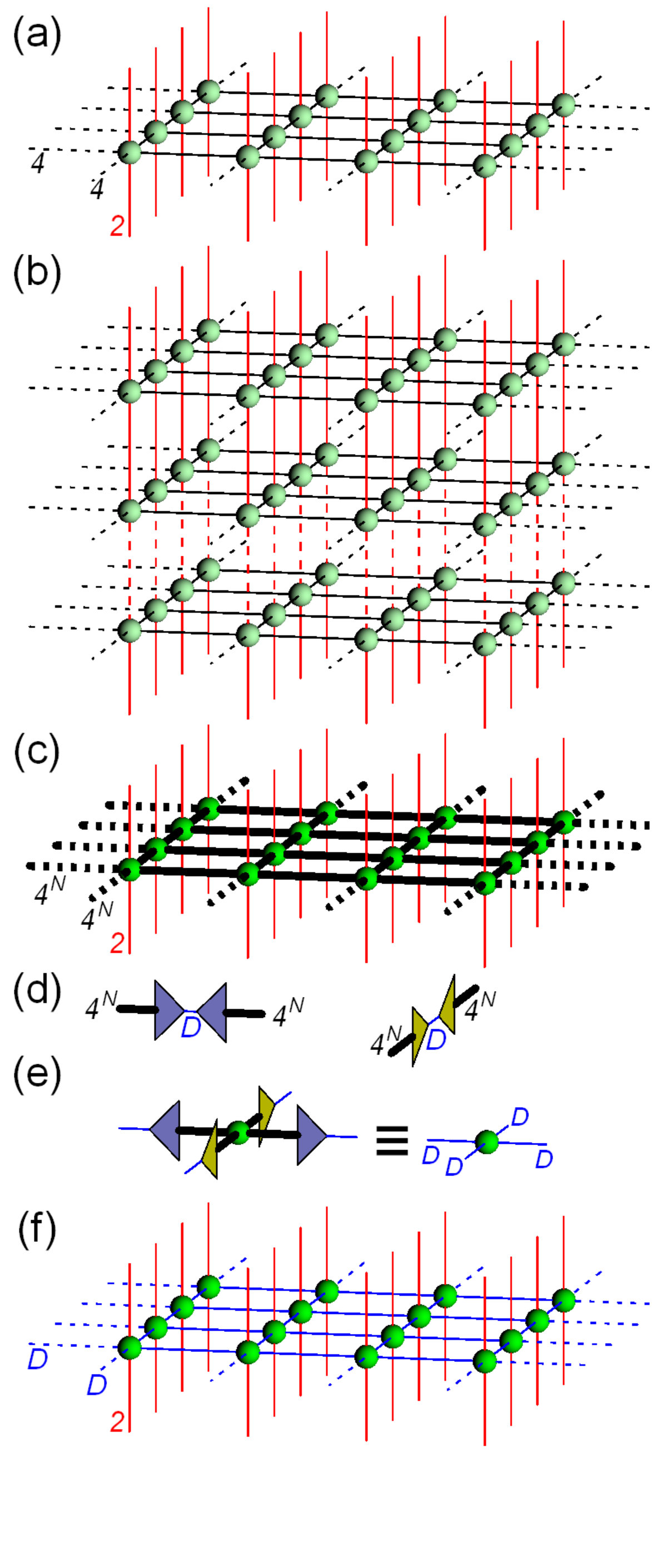 Figure 1
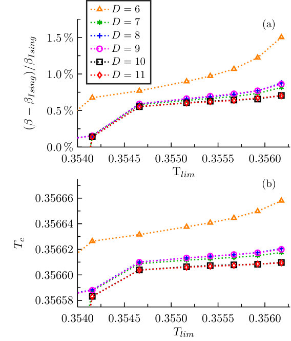 Figure 2
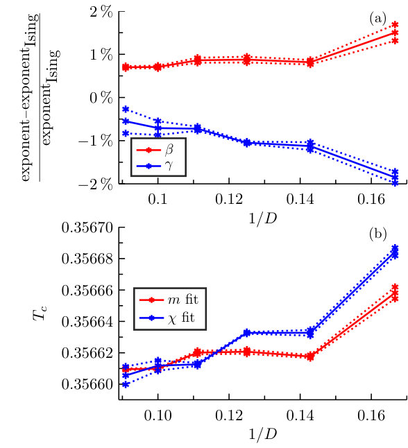 Figure 3
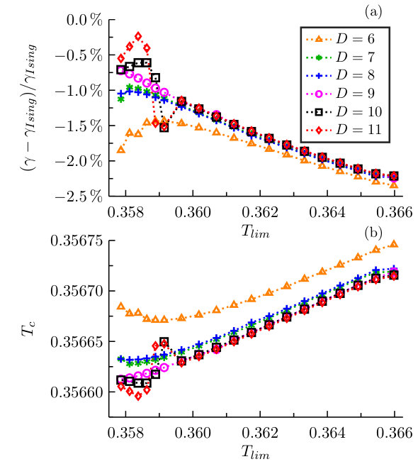 Figure 4
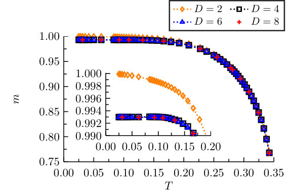 Figure 5
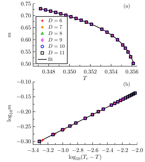 Figure 6
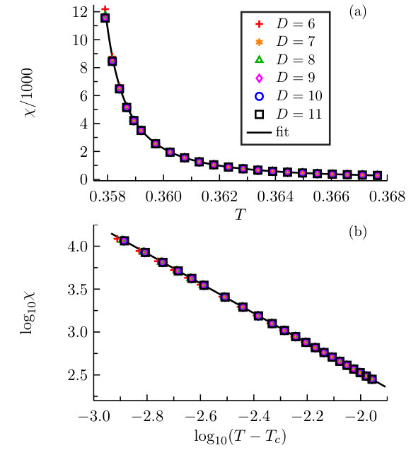 Figure 7
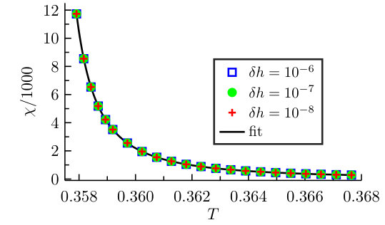 Figure 8
| 0.356631 | 1.7324 | |||
| 0.356633 | 1.7317 | |||
| 0.356633 | 1.7317 |
Peer Reviews
No public reviews on file for this paper yet. If you reviewed it on a platform where reviews are public (OpenReview, ICLR, NeurIPS, ICML), you can paste yours below so the community can read it here.
Videos
No videos yet. Explain this paper in a talk, walkthrough, or lecture? Add one.
Overcoming the sign problem at finite temperature:
Quantum Tensor Network for the orbital model on an infinite square lattice
Piotr Czarnik
Instytut Fizyki im. Mariana Smoluchowskiego, Uniwersytet Jagielloński, prof. S. Łojasiewicza 11, PL-30-348 Kraków, Poland
Institute for Theoretical Physics, Universiteit van Amsterdam, Science Park 904, NL-1098 XH Amsterdam, The Netherlands
Jacek Dziarmaga
Instytut Fizyki im. Mariana Smoluchowskiego, Uniwersytet Jagielloński, prof. S. Łojasiewicza 11, PL-30-348 Kraków, Poland
Andrzej M. Oleś
Instytut Fizyki im. Mariana Smoluchowskiego, Uniwersytet Jagielloński, prof. S. Łojasiewicza 11, PL-30-348 Kraków, Poland
Max-Planck-Institut für Festkörperforschung, Heisenbergstrasse 1, D-70569 Stuttgart, Germany
Abstract
The variational tensor network renormalization approach to two-dimensional (2D) quantum systems at finite temperature is applied for the first time to a model suffering the notorious quantum Monte Carlo sign problem — the orbital model with spatially highly anisotropic orbital interactions. Coarse-graining of the tensor network along the inverse temperature yields a numerically tractable 2D tensor network representing the Gibbs state. Its bond dimension — limiting the amount of entanglement — is a natural refinement parameter. Increasing we obtain a converged order parameter and its linear susceptibility close to the critical point. They confirm the existence of finite order parameter below the critical temperature , provide a numerically exact estimate of , and give the critical exponents within of the 2D Ising universality class.
[Published in: Physical Review B 96, 014420 (2017)]
I Introduction
Frustration in quantum spin systems occurs by competing exchange interactions and often leads to disordered spin liquids Bal10 ; Lucile . This is in contrast to Ising spins on a square lattice where periodically distributed partial frustration in form of exchange interactions with different signs does not suppress a phase transition at finite temperature Lon80 , while complete frustration gives a disordered classical phase Vil77 . Frustration may also be generated by a different mechanism — when Ising-like interactions for different pseudospin components compete on a square lattice in the two-dimensional (2D) compass model Nus05 ; Dou05 ; Dor05 ; Tro10 or on the honeycomb lattice in the Kitaev model Kit06 . While the short-range spin liquid is realized in the Kitaev model Bas07 , the pseudospin nematic order stabilizes below in the 2D compass model Wen10 ; Cza16 . In such cases entanglement plays an important role Ami08 and advanced methods of quantum many-body theory have to be applied.
In real systems pseudospin interactions concern the orbital degrees of freedom. The case of orbitals is paradigmatic here as it (i) is related to the 2D compass model Cin10 and (ii) initiated spin-orbital physics Kug82 ; Fei97 ; Tok00 ; Cor12 ; Brz15 — the well known systems with orbitals are: KCuF3 Bella ; Dei08 ; Pav08 , LaMnO3 Dag01 ; Fei99 ; Ish02 ; Ish03 ; Ole05 ; Pav10 ; Kov10 ; Sna16 , and LiNiO2 Rey01 ; Mil04 ; Rei05 . This field is very challenging due to the interplay and entanglement of spins and orbitals which leads to remarkable consequences Ole12 ; Brz12 . However, when spin order is ferromagnetic, as in the planes of KCuF3 and LaMnO3, spins disentangle and one is left with the 2D orbital model vdB99 ; Tan05 where hole propagation is possible by the coupling to orbitons vdB00 . Surprisingly, the tendency towards long-range order with such excitations is then opposite to that for spin systems Mat06 , i.e., orbital order occurs in a 2D square lattice below Ryn10 ; Wen11 , for instance in K2CuF4 kcuf4 ; Mos04 , while the role of quantum fluctuations increases with increasing dimension vdB99 ; Fei05 .
In this article we investigate a phase transition at in the 2D orbital model. A better understanding of the signatures of this phase transition provides a theoretical challenge. We present a very accurate estimate of and the critical exponents being in the 2D Ising universality class. These results could be achieved due to a remarkable recent progress in tensor networks due to the formulation of an algorithm at finite temperature using a projected entangled-pair operator (PEPO) var .
The paper is organized as follows. Sec. II gives brief overview of tensor network methods. Sec. III introduces simulated model. Sec. IV introduces 2D finite temperature tensor network method used to simulate the model. Numerical results are presented in Sec. V. Sec. VI summarizes the paper. Appendix A gives detailed description of results convergence analysis which enabled us to obtain trustworthy results for the model. Technical details of simulations are given in Appendix B. Finally Appendix C gives additional results for low temperature regime of the model.
II Tensor networks
Since the discovery of the density matrix renormalization group (DMRG) White ; Sch05 — that was later shown to optimize the matrix product state (MPS) variational ansatz Sch11 — quantum tensor networks proved to be an indispensable tool to study strongly correlated quantum systems Che15 . MPS ansatz was later generalized to a 2D projected entangled pair state (PEPS) PEPS ; CMRPEPS and supplemented with the multiscale entanglement renormalization ansatz (MERA) MERA . The networks do not suffer from the notorious sign problem fermions and in the doped case fermionic PEPS provided better variational energies for the - model PEPStJ and the Hubbard model Cor15 than the best available variational Monte Carlo results. A combination of different tensor networks, supplemented with other sign-error free methods, seems to have finally settled the controversy on the ground state of the underdoped Hubbard model stripesHubbard . The networks — both MPS Yan11 ; Cin13 ; Ran15 and PEPS Poi12 ; Poi13 ; Wan13 — also made some major breakthroughs in the search for topological order. This is where, like in the model Ryn10 , geometric frustration often prohibits the traditional quantum Monte Carlo.
Thermal states of quantum Hamiltonians were explored much less than their ground states. In one dimension they can be represented by an MPS ansatz prepared with an accurate imaginary time evolution Ver04 ; WhiteT . A similar approach can be applied in 2D models Czarnik ; self , where the PEPS manifold is a compact representation for Gibbs states Molnar but the accurate evolution proved to be more challenging. Alternative direct contractions of the 3D partition function were proposed ChinaT but, due to local tensor update, they are expected to converge more slowly with increasing refinement parameter. Even a small improvement towards a full update can accelerate the convergence significantly HOSRG .
In order to avoid these problems, in the pioneering work var two of us introduced an algorithm to optimize variationally a projected entangled-pair operator (PEPO) representing the Gibbs state of a 2D lattice system (). Its first challenging benchmark applications include the quantum compass Cza16 and Hubbard varHubbard models where it provided accuracy comparable to the best conventional methods.
It was not quite unexpected. Just like for the ground-state PEPS, the accuracy of the thermal PEPO is limited by its finite bond dimension , i.e., the size of tensor indices connecting nearest-neighbor lattice sites. This size limits the entanglement within the ground/thermal state. However, by its very definition the Gibbs state is the mixed state that maximizes the entropy for a given average energy. Since this maximal entropy is actually the entropy of entanglement with the rest of the universe, then — thanks to the monogamy of entanglement — the Gibbs state also minimizes its internal entanglement. Among all states with the same average energy it is the one most suited to be represented by a tensor network. Encouraged by the benchmarks tests, in this work we apply the algorithm for the first time to a model that evades treatment by quantum Monte Carlo Ryn10 ; Wen11 . Numerical convergence and self-consistency alone allow us to make definitive statements on the physics of the model demonstrating the power of this method.
III The orbital model
The quantum model on an infinite square lattice is defined by the Hamiltonian
[TABLE]
Here labels lattice sites, are unit vectors along the axis and are orbital operators represented by Pauli matrices:
[TABLE]
The coupling in the orbital space depends on the spatial orientation of the bond. In what follows .
At low temperature a spontaneous breaking of symmetry takes place and the system orders according to the strongest interaction Cin10 . This symmetry breaking implies a finite real order parameter
[TABLE]
Unlike the 2D compass model Wen10 , the model (1) is not tractable by Monte Carlo Wen11 , but the order parameter suggests the 2D Ising universality class for the finite temperature transition which is confirmed by our simulations.
IV The algorithm at
The algorithm was described in all technical detail elsewhere Cza16 . Its aim is to represent matrix elements of the operator by the 2D tensor network in Fig. 1. Here we show only a small unit of an infinite square lattice and each geometrical shape (here a green ball) represents a tensor. There is one tensor at every lattice site. Each line sticking out of the tensor represents one index. A (black) line connecting two tensors represents a tensor contraction through the connecting index. There is one bond index along every nearest neighbor bond. It has a finite bond dimension . The dashed bond lines connect the unit with the rest of the lattice. The open (red) vertical indices number the orbital basis’ states. Those pointing up/down number bra/ket states. The desired 2D network in Fig. 1(f) — known as PEPO — can be contracted efficiently to obtain local expectation values. A finite is sufficient to represent Gibbs states with their limited entanglement.
On the other hand, the 2D operator can be naturally represented by a 3D network, the third dimension being the imaginary time . The evolution is split into small time steps (), . With a Suzuki-Trotter decomposition, each step can be represented by a 2D layer in Fig. 1(a). In the model, its bond indices have dimension . The product of steps is the 3D network in Fig. 1(b). Here we show only three layers; the remaining ones are represented by the vertical dashed lines.
The 3D network is too hard to treat directly. Formally, it can be compressed to a 2D network by contracting along each vertical column first. The resulting 2D network in Fig. 1(c) arises at the price of a huge bond dimension . Fortunately, we know that just a tiny -dimensional subspace in the dimensions is enough to accommodate all correlations. Therefore, it is justified to insert every bond line with a -dimensional projection made of two isometries. There are two independent projections along the axes and , see Fig. 1(d). After the insertion, every isometry is absorbed into its nearest tensor truncating its bond index down to a tractable size , see Fig. 1(e). The outcome is the desired PEPO in Fig. 1(f), and the Gibbs state is .
Now the problem is how to handle the huge isometries from to . Fortunately, by a divide-and-conquer strategy, each of them can be split into a hierarchy of smaller isometries connected into a tree tensor network Cza16 . It is possible to optimize the smaller isometries one-by-one to obtain the most accurate projection available for a given . The cost of the algorithm is polynomial in and only logarithmic in the number of steps , allowing for small enough to make the Suzuki-Trotter decomposition numerically exact at very little expense.
V Numerical Results
For each the order parameter (3) was converged in in the symmetry broken phase, see Fig. 2. For each it was fitted with a power law,
[TABLE]
see Fig. 3. Here is the order-parameter critical exponent (not to be confused with the inverse temperature ). For the estimates: , and , do not depend significantly on increasing . They slowly drift towards and , respectively. For more details see Appendix A.
In the symmetric phase above , we calculated the magnetic susceptibility using the linear approximation,
[TABLE]
Here is an infinitesimal symmetry-breaking field added to the Hamiltonian (1). The derivative was approximated accurately by a finite difference between and . More details on numerical calculation are given in Appendix B, see Fig. 7 and Table 1.
The susceptibility was converged in (Fig. 4) and fitted with a power law,
[TABLE]
see Fig. 3 and Appendix A. Again, for the estimates: , and , almost do not depend on increasing , and drift towards and . Altogether, both exponents are less than away from the exact [see Fig. 5(a)] and in the 2D Ising universality class.
Remarkably, found from (4) and (6) is identical up to the four-digit precision. We propose
[TABLE]
deduced from the scatter of the data for in Fig. 3(b) multiplied by a factor of , see also Fig. 5(b). It is worthwhile to compare the above estimate (7) with the 2D Ising model Ons44 with interaction ,
[TABLE]
Exchange interactions in the dominating term in Eq. (1) are reduced by the factor from the 2D Ising model, so this reduction alone would give instead . De facto, the obtained value in Eq. (7) is , i.e., it is further reduced by % by quantum fluctuations activated at finite due to and terms in Eq. (1). The order parameter (3) at is almost saturated as quantum fluctuations are negligible at ,
[TABLE]
More details on simulation are given in Appendix C, see Fig. 8. The value in Eq. (9) was obtained by the present method and agrees with the ground state MERA calculations Cin10 . This shows that the quantum fluctuation effects in the orbital model (1) are very weak indeed at vdB99 , while at the fluctuations are activated and reduce significantly the value of the critical temperature down to , see Eq. (7). Indeed quantum fluctuations play a role here but are not as significant as for the 2D SU(2) symmetric Heisenberg antiferromagnet Mat06 . Yet, the entanglement between the orbital operators is here much reduced from that in the 2D compass model var and therefore such an accurate estimate of (7) is possible.
VI Summary
Being a paradigmatic frustrated system, the orbital model evades treatment by quantum Monte Carlo but it proves to be accurately tractable by our thermal tensor network. The notorious sign problem — often inescapable for quantum Monte Carlo — is not an issue for our method. Instead the relevant issue is if the entanglement in a thermal state can be accommodated within a bond dimension that is small enough to fit into a classical computer. This criterion is satisfied by the thermal state of the model and a four-digit estimate of the critical temperature and a better than accuracy of the critical exponents could be achieved. Since the Gibbs state is the least entangled one among all excited states with the same average energy, it is potentially the easiest target for a suitable tensor network.
Acknowledgements.
We thank Philippe Corboz for insightful discussions. We kindly acknowledge support by Narodowe Centrum Nauki (NCN, National Science Centre, Poland) under Projects: No. 2013/09/B/ST3/01603 (P.C. and J.D.) and No. 2016/23/B/ST3/00839 (A.M.O.). The work of P.C. on his Ph.D. thesis was supported by NCN under Project No. 2015/16/T/ST3/00502.
Appendix A Convergence of the results
The bond dimension (see Fig. 1) has to be large enough to accommodate the entanglement in the thermal state. Furthermore, an environmental bond dimension that is used in the analysis of the effective 2D tensor network depicted in Fig. 1(f) (see Ref. Cza16 for details) has to be large enough to accommodate long range correlations. In general, these requirements cannot be satisfied at the critical temperature but the phase transition can be approached from both sides close enough to fit the critical power laws. In this appendix we demonstrate that indeed we are able to approach close enough to obtain stable and converged fits.
All results presented here, which were obtained with , are converged in . Another potential source of errors are Trotter errors. They are not a significant issue for our approach as its cost scales at most logarithmically with the the inverse Trotter time step . Our results were obtained with and are converged in .
The convergence of the critical exponents, for the magnetization and for the susceptibility , is shown in Figs. 5(a) and 6(a) where we compare them with the 2D Ising model exponents,
[TABLE]
For we see that the exponents approach the Ising values while is approaching . For sufficiently close to they no longer depend significantly on range of depending instead primarily on . In this regime all fitted exponents fall within of 2D Ising universality class, drifting towards or with increasing . The obtained behavior of the exponents indicates the 2D Ising universality class of the transition.
The data collected in Figs. 5(b) and 6(b) demonstrate similar convergence behavior of fitted as for the exponents. For fitted approaches when is approaching the critical point. For sufficiently close to the critical point begins to depend primarily on rather than on . Reaching this regime where the fits become stable with respect to justifies taking into account only their dependence to obtain the final estimate Eq. (7).
We remark that our estimate of is based on two independent estimates, coming either from the or fits, which agree up to five digits for the largest .
Appendix B Numerical details
In our simulations we use the algorithm described in detail in Ref. Cza16 . In prticular we use corner matrix renormalization (CMR) to contract approximately tensor networks representing thermal states CMR ; CMRPEPS . To reach convergence of the observables and approximately iterations of the optimization loop were necessary. The isometries at the beginning of the loop were initialized by a local truncation scheme based on higher-order singular value decomposition. The CMR procedure made iterations in the whole loop. The further away from the phase transition, the fewer CMR iterations were necessary to reach convergence.
Linear susceptibility defined by Eq. (5) was calculated from a finite difference of the order parameter corresponding to finite difference of the symmetry breaking field :
[TABLE]
where . Fig. 7 shows that is already converged in for . More accurate benchmark of convergence is given by Table 1 showing that decreasing further results in changes of fitted and that are negligible as compared to their dependence on or the range of .
All simulations were done in Matlab with an extensive use of the Ncon procedure encon . To give an idea of the actual time and computer resources needed to generate the data, the most challenging data points nearest to the phase transition, with the largest bond dimensions and , required days on a desktop.
Appendix C Simulation of the low temperature phase
The entanglement in the low phase is small enough to converge the curve in already for , see Fig. 8.
Thanks to a short correlation length at low temperature, the calculations are much less demanding numerically than close to the critical point. Because of that we were able to generate the data shown in Fig. 8 during one day using a laptop.
The reference list from the paper itself. Each links out to its DOI / PubMed record.
- 1(1) Leon Balents, Nature (London) 464 , 199 (2010).
- 2(2) Lucile Savary and Leon Balents, Rep. Progr. Phys. 80 , 016502 (2017).
- 3(3) L. Longa and A. M. Oleś, J. Phys. A: Math. Theor. 13 , 1031 (1980).
- 4(4) J. Villain, J. Phys. C: Solid State Phys. 10 , 1717 (1977).
- 5(5) Z. Nussinov and E. Fradkin, Phys. Rev. B 71 , 195120 (2005).
- 6(6) B. Douçot, M. V. Feigel’man, L. B. Ioffe, and A. S. Ioselevich, Phys. Rev. B 71 , 024505 (2005).
- 7(7) J. Dorier, F. Becca, and F. Mila, Phys. Rev. B 72 , 024448 (2005).
- 8(8) F. Trousselet, A. M. Oleś, and P. Horsch, Europhys. Lett. 91 , 40005 (2010); Phys. Rev. B 86 , 134412 (2012); W. Brzezicki and A. M. Oleś, ibid. 82 , 060401 (2010); 87 , 214421 (2013).