Imaging polarizable dipoles
Maxence Cassier, Fernando Guevara Vasquez

TL;DR
This paper develops an electromagnetic imaging method for polarizable dipoles, providing resolution estimates and error analysis, and addresses artifacts in the imaging process with numerical validation.
Contribution
It introduces a Kirchhoff imaging approach for electromagnetic dipoles, analyzing resolution and errors, and extends to active imaging of scatterers' polarizability tensors.
Findings
Range and cross-range resolution match acoustic estimates.
Error bounds for dipole orientation reconstruction are established.
Naive imaging methods suffer from artifacts, which are characterized and corrected.
Abstract
We present a method for imaging the polarization vector of an electric dipole distribution in a homogeneous medium from measurements of the electric field made at a passive array. We study an electromagnetic version of Kirchhoff imaging and prove, in the Fraunhofer asymptotic regime, that range and cross-range resolution estimates are identical to those in acoustics. Our asymptotic analysis provides error estimates for the cross-range dipole orientation reconstruction and shows that the range component of the dipole orientation is lost in this regime. A naive generalization of the Kirchhoff imaging function is afflicted by oscillatory artifacts in range, that we characterize and correct. We also consider the active imaging problem which consists in imaging both the position and polarizability tensors of small scatterers in the medium using an array of collocated sources and receivers.…
Click any figure to enlarge with its caption.
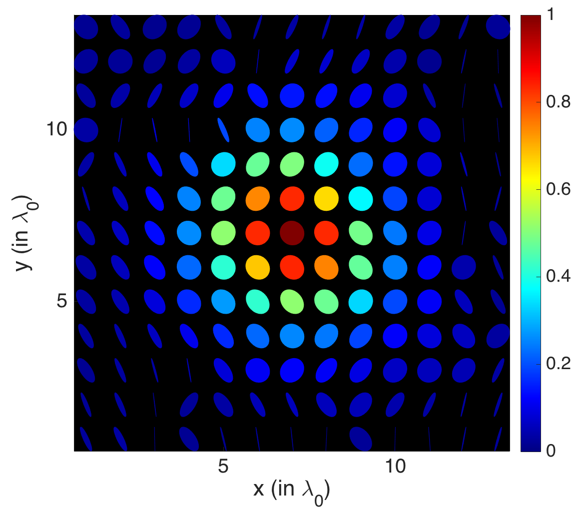 Figure 1
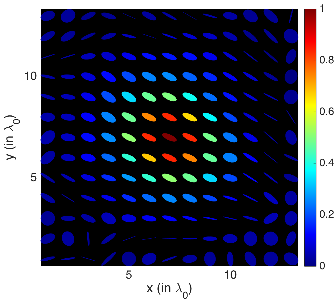 Figure 2
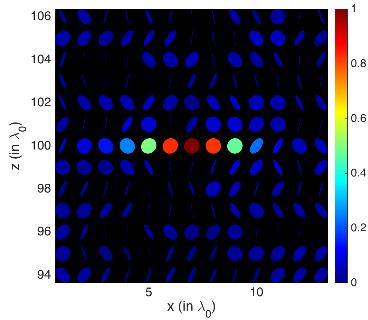 Figure 3
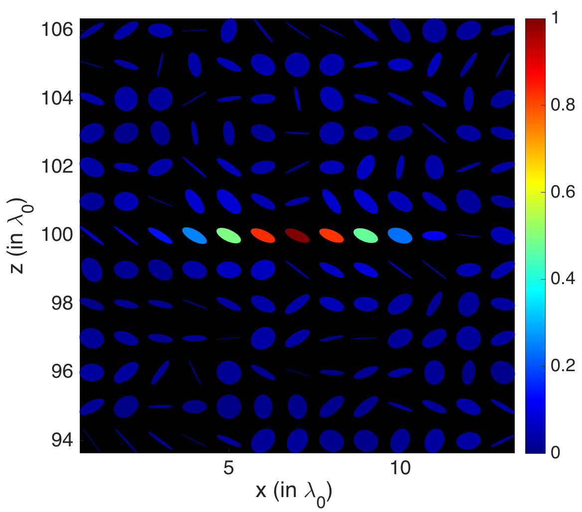 Figure 4
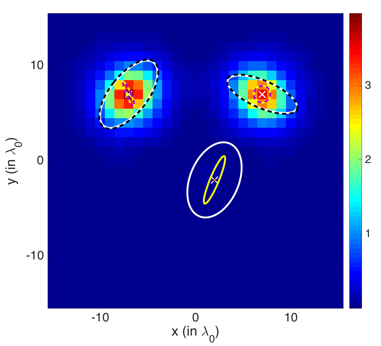 Figure 5
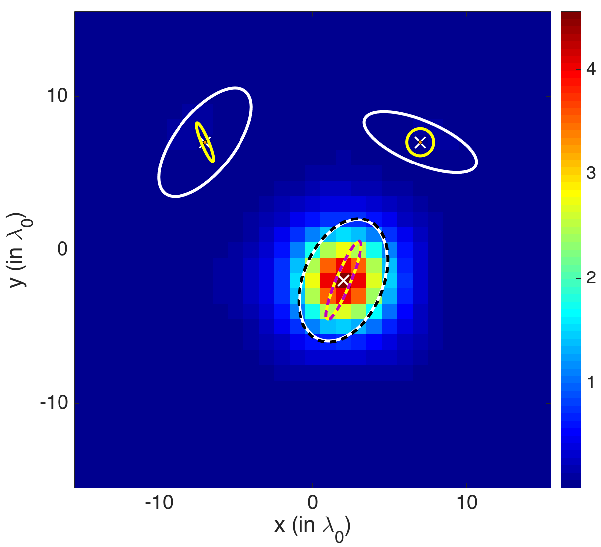 Figure 6
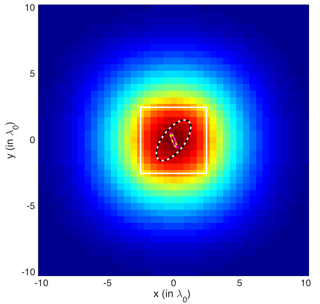 Figure 7
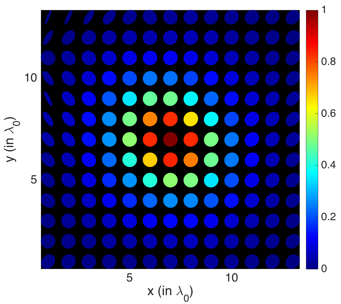 Figure 8
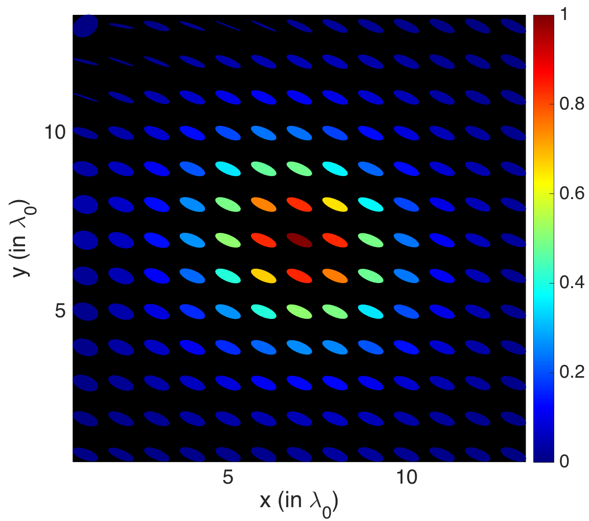 Figure 9
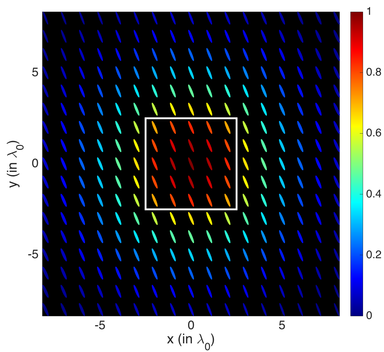 Figure 10
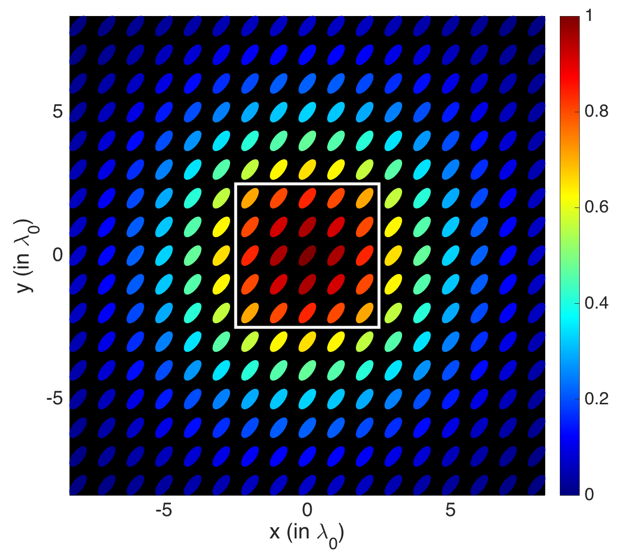 Figure 11
 Figure 12
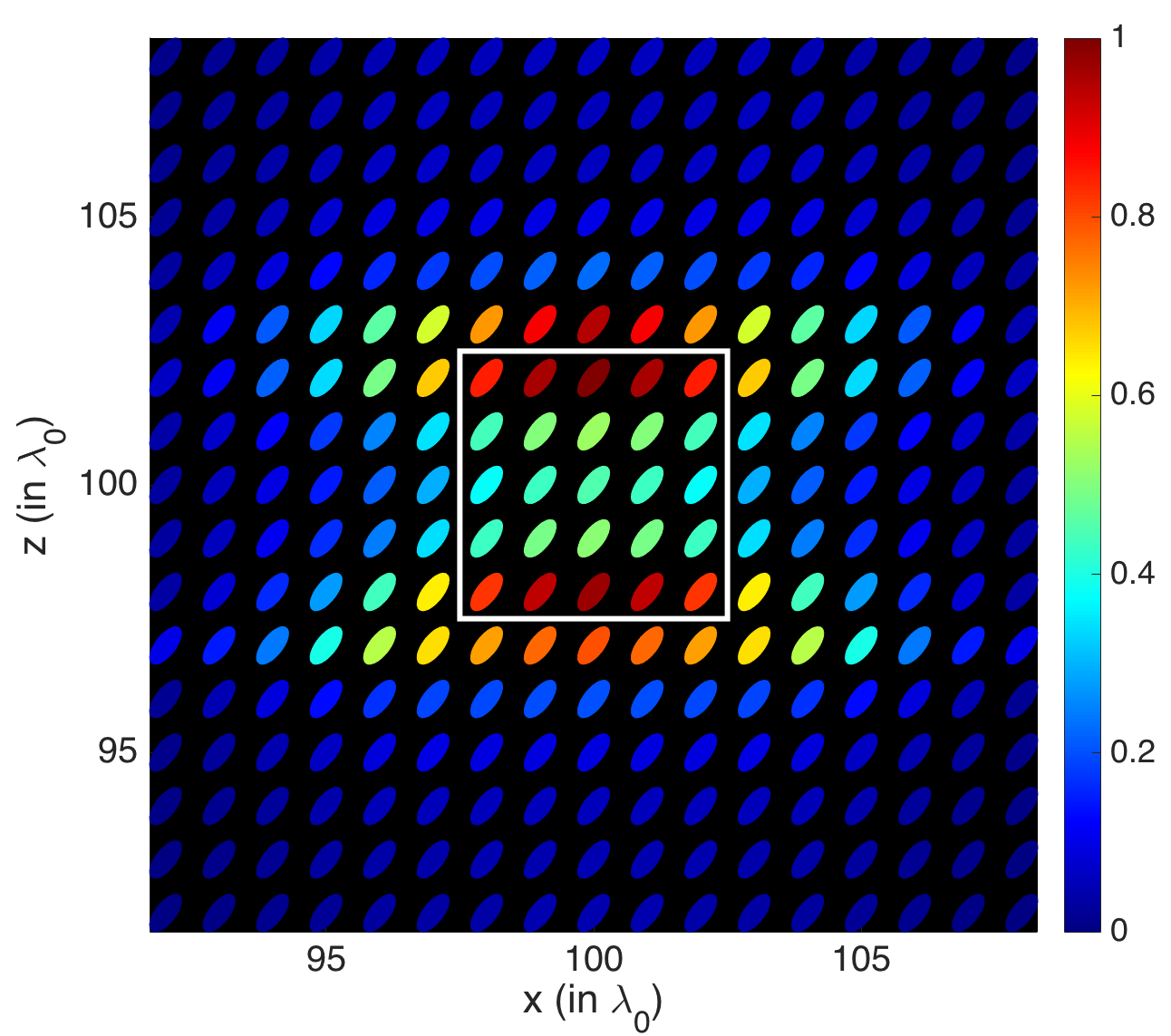 Figure 13
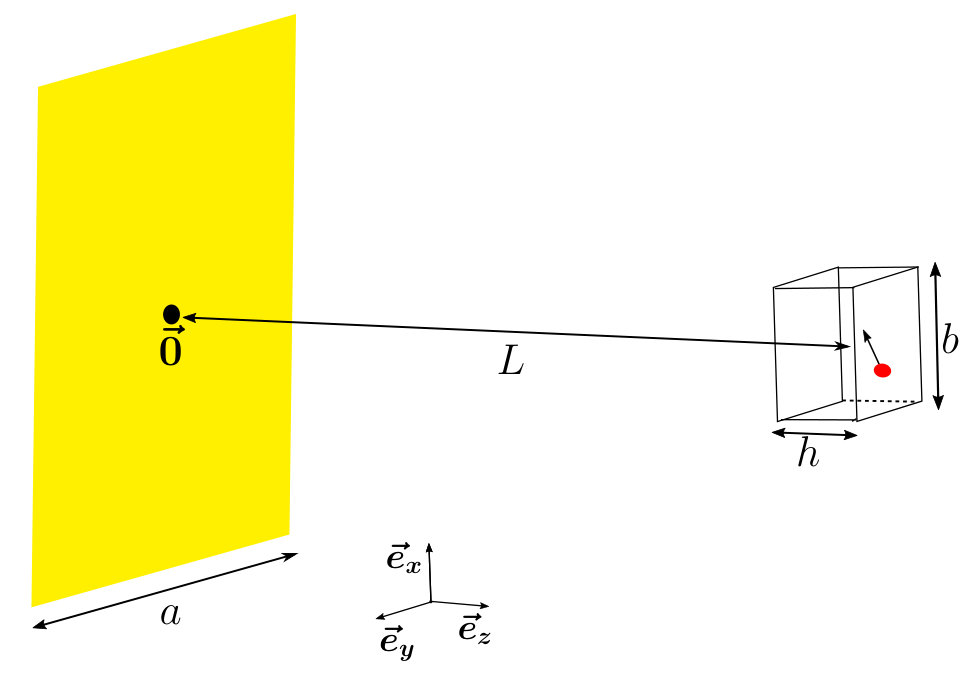 Figure 14
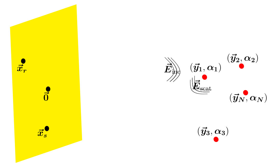 Figure 15
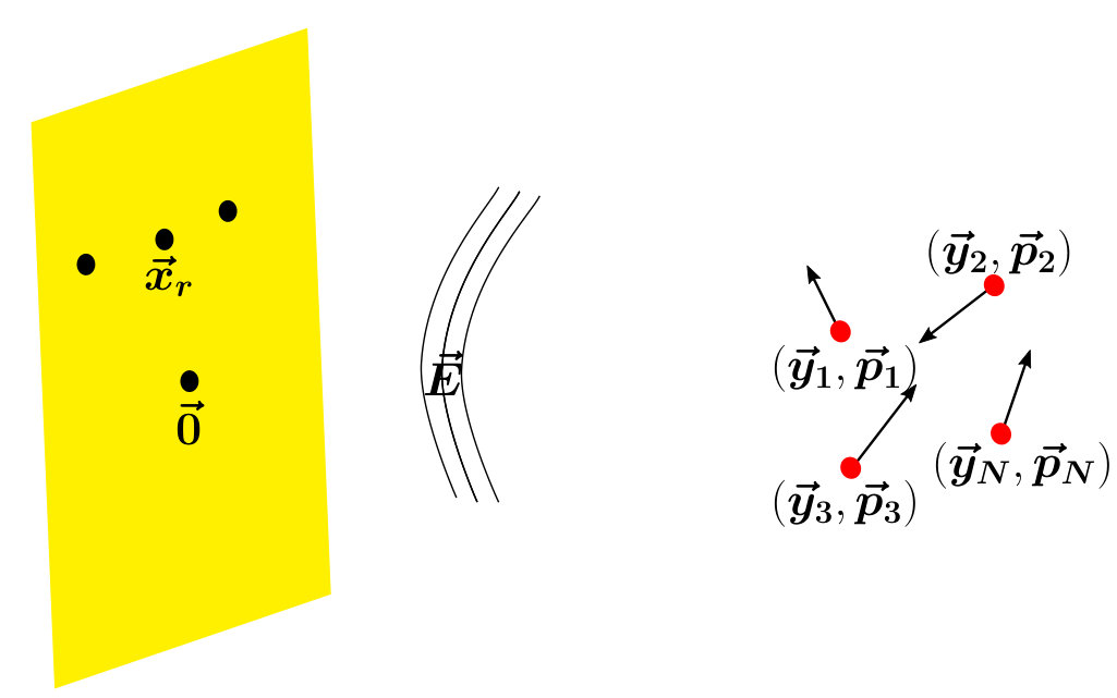 Figure 16
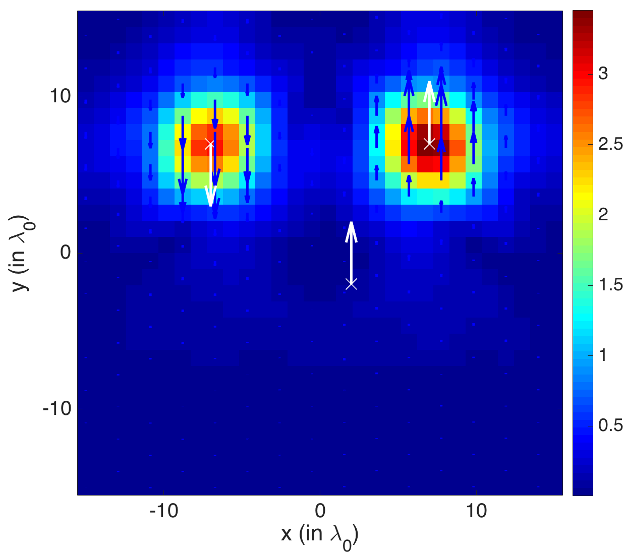 Figure 17
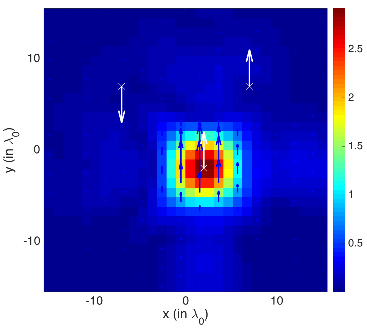 Figure 18
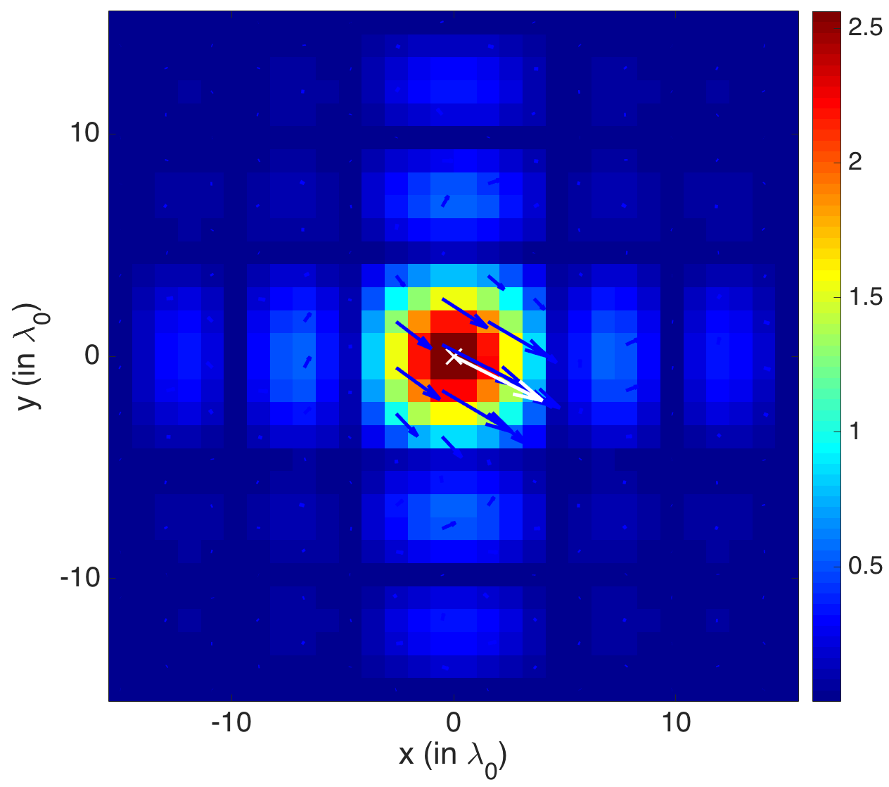 Figure 19
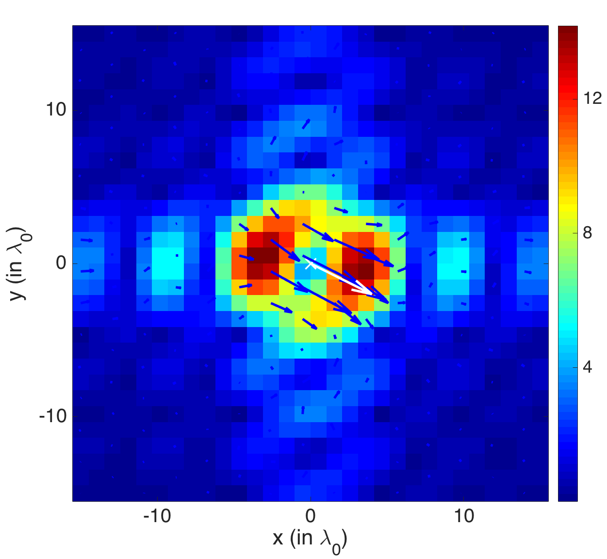 Figure 20
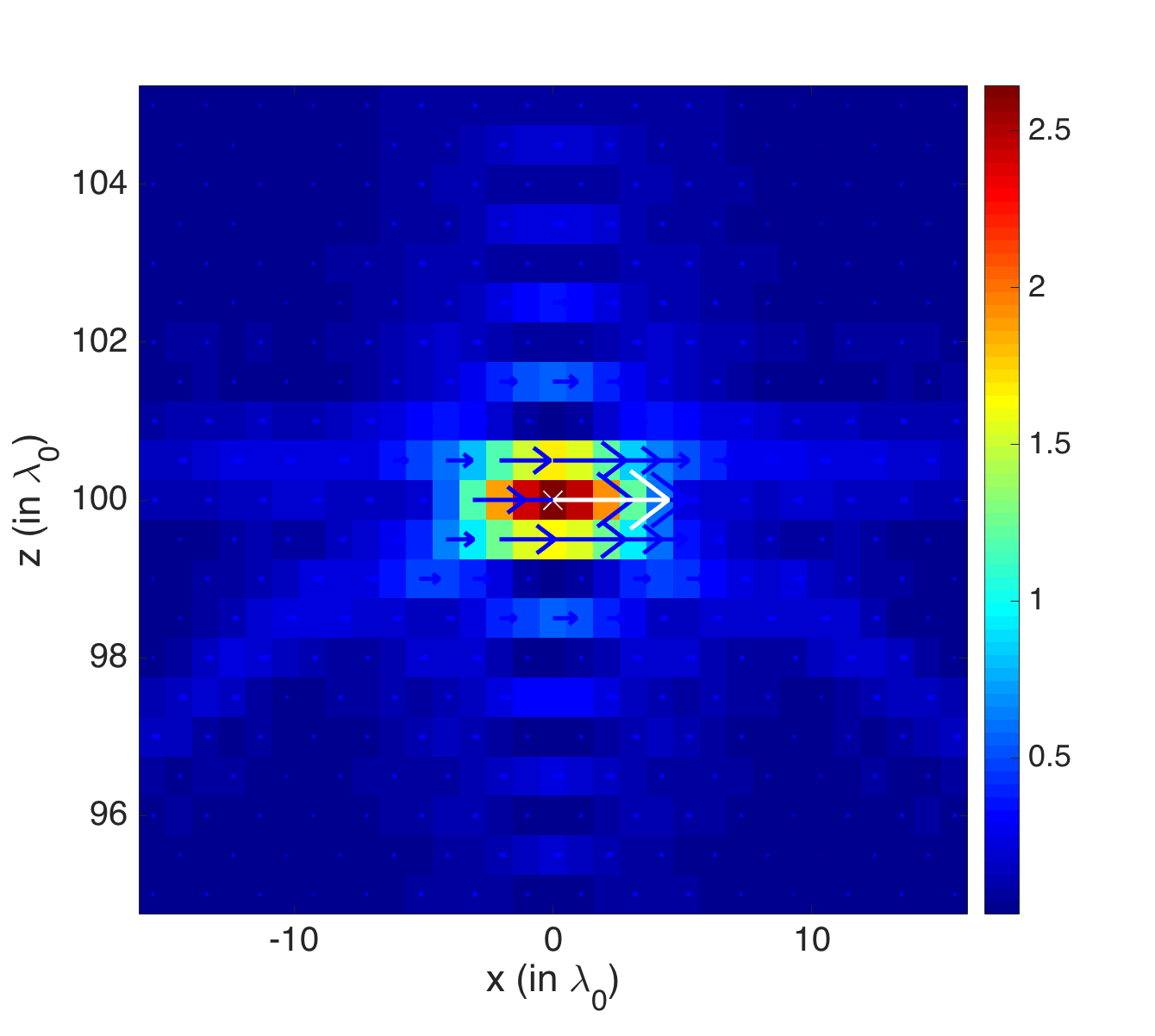 Figure 21
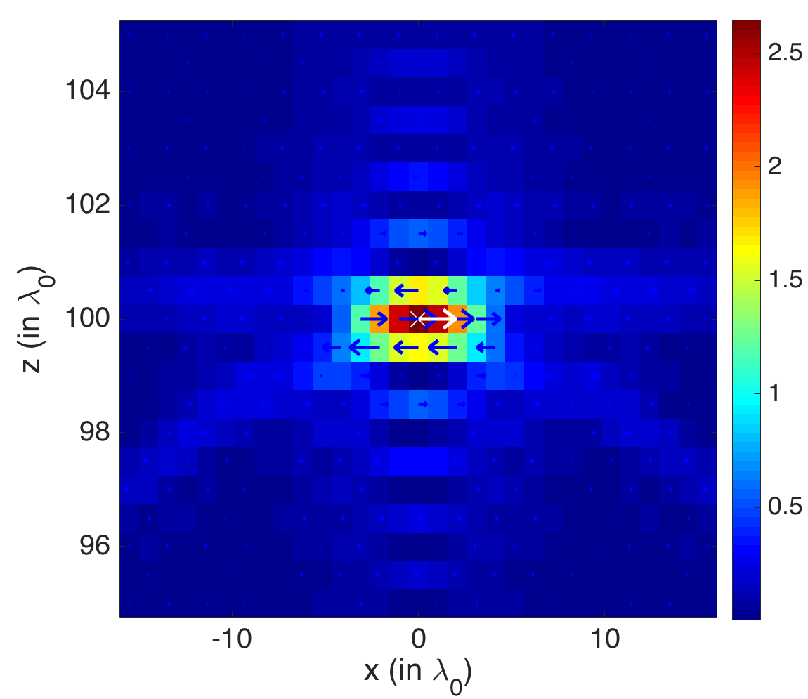 Figure 22
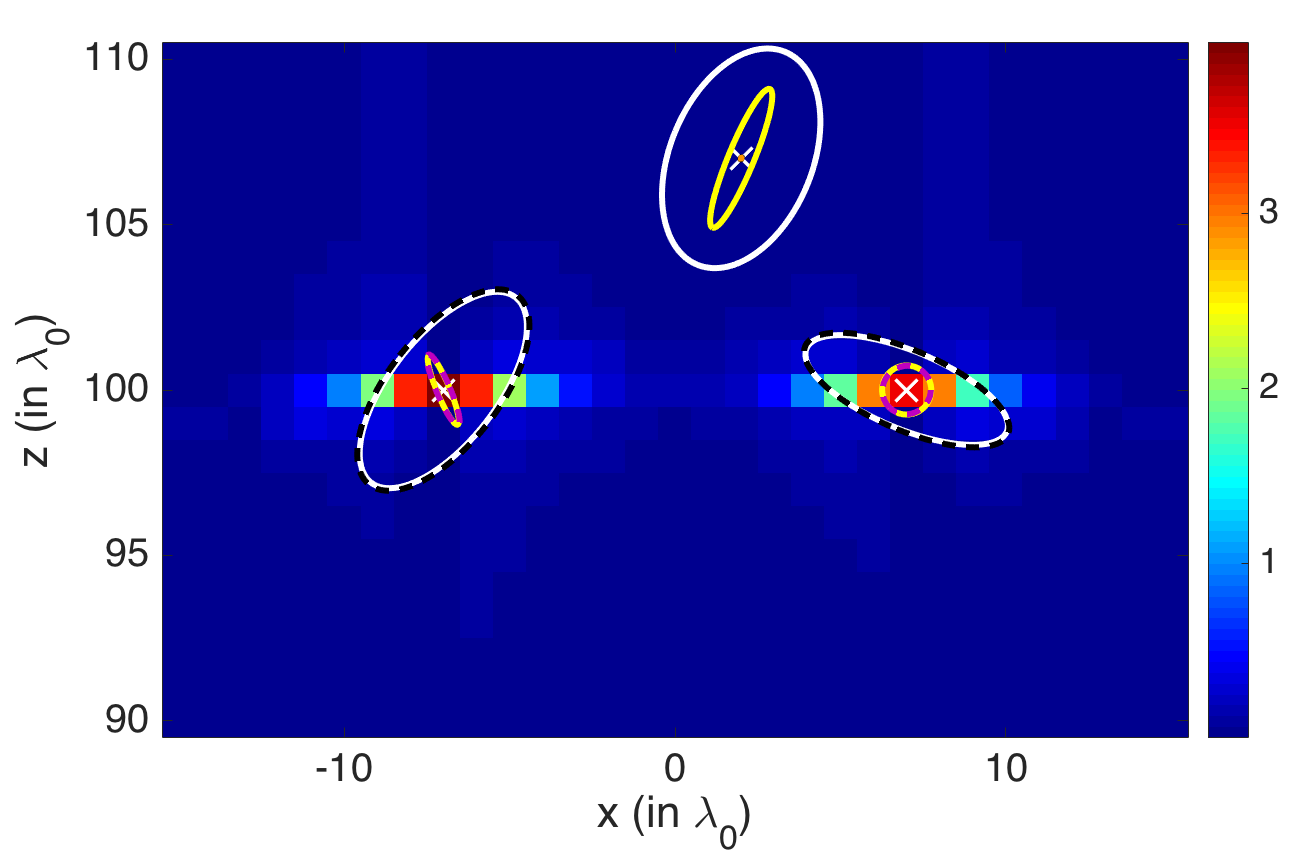 Figure 23
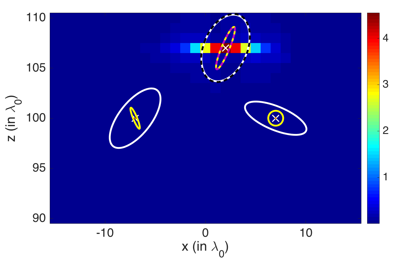 Figure 24
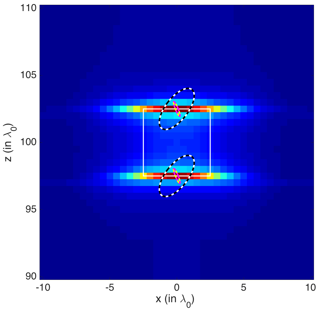 Figure 25
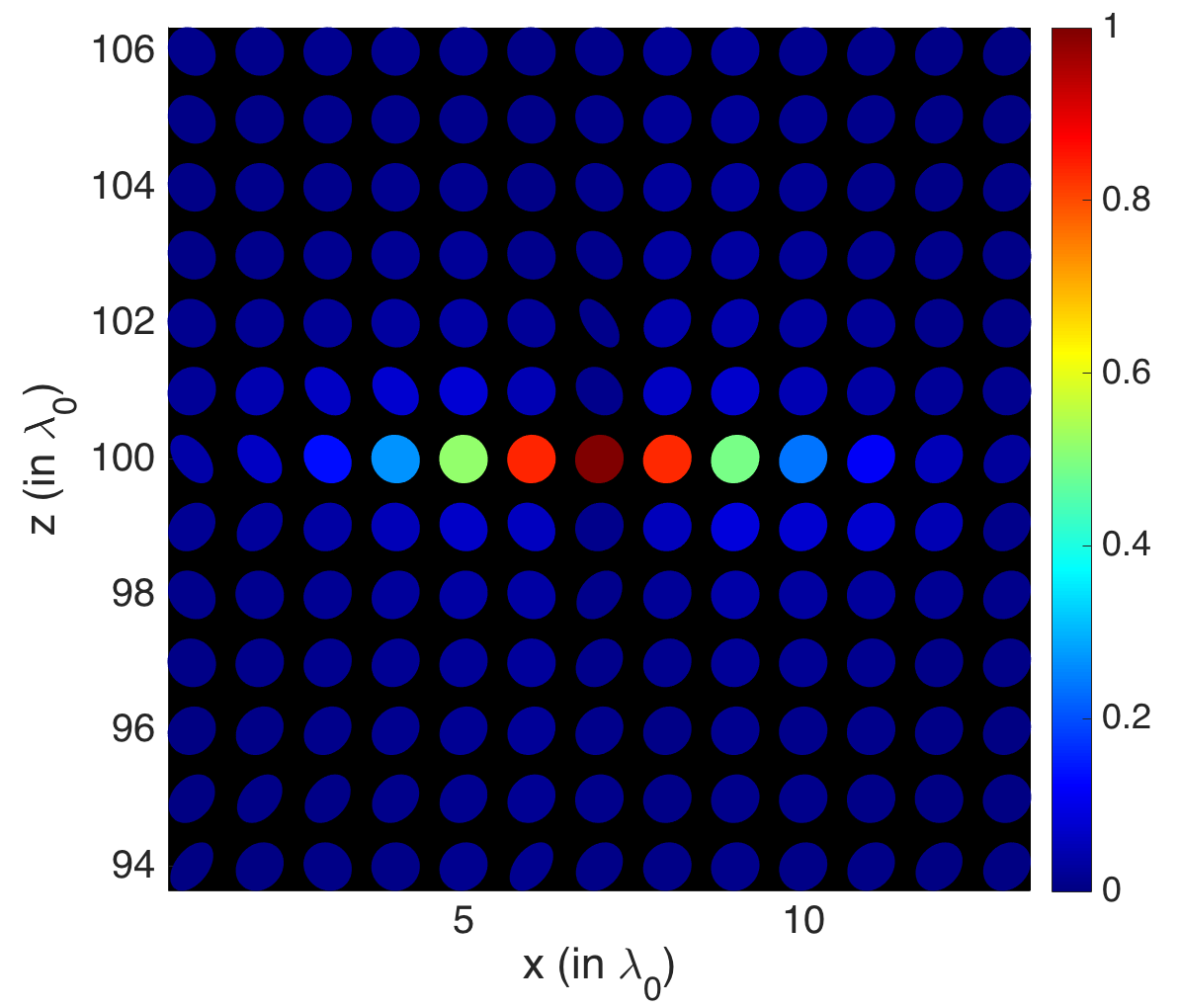 Figure 26
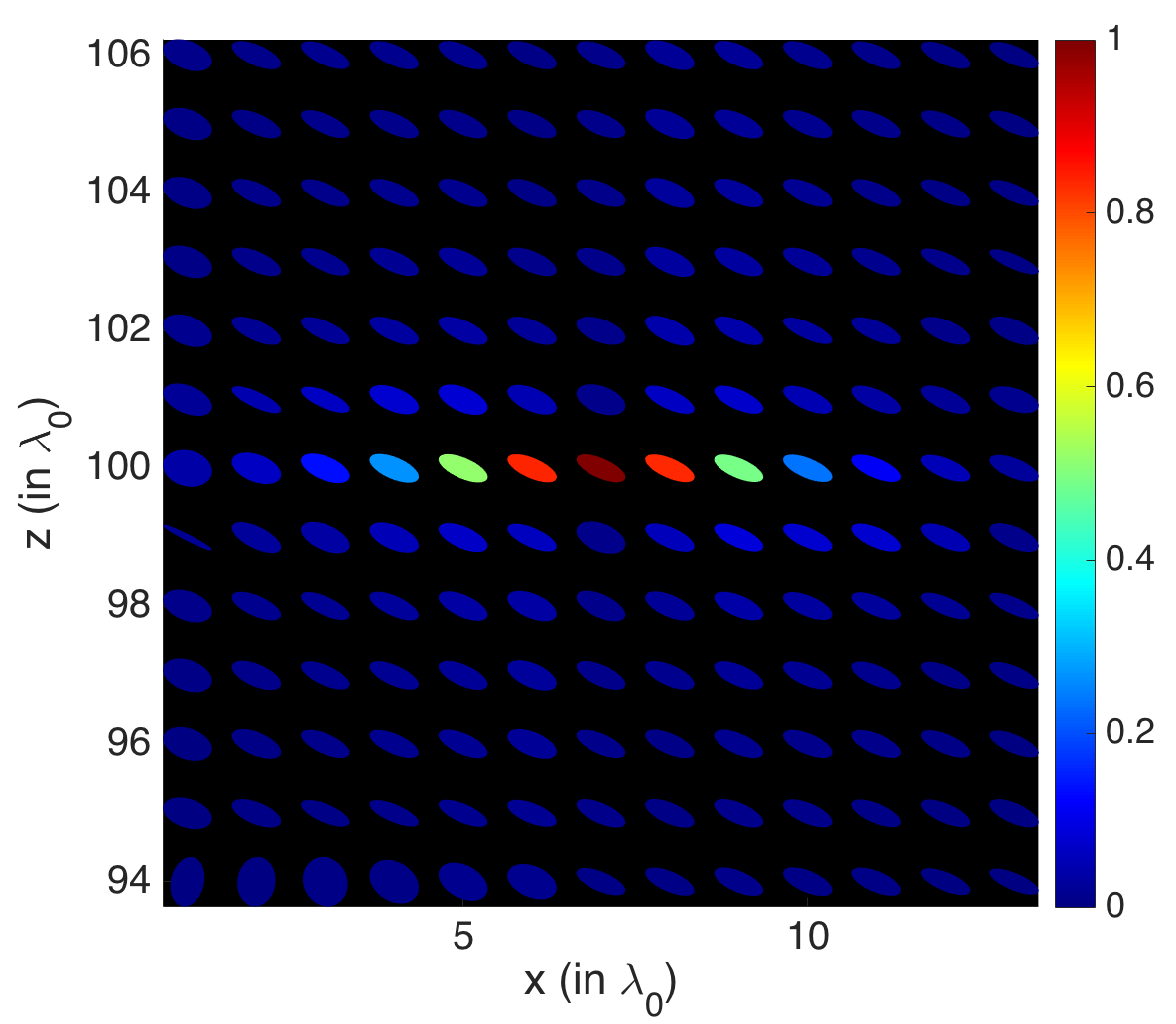 Figure 27
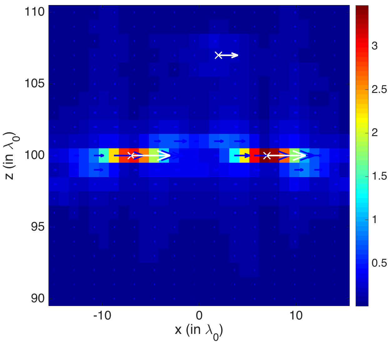 Figure 28
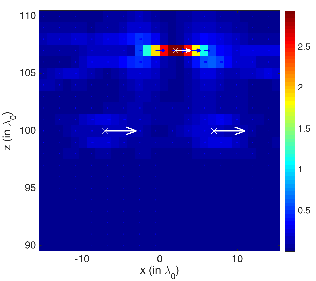 Figure 29
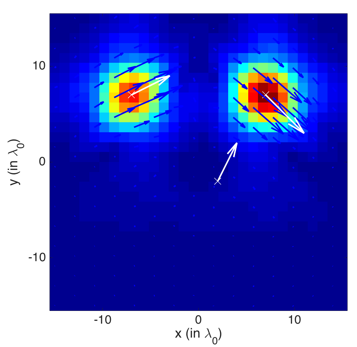 Figure 30
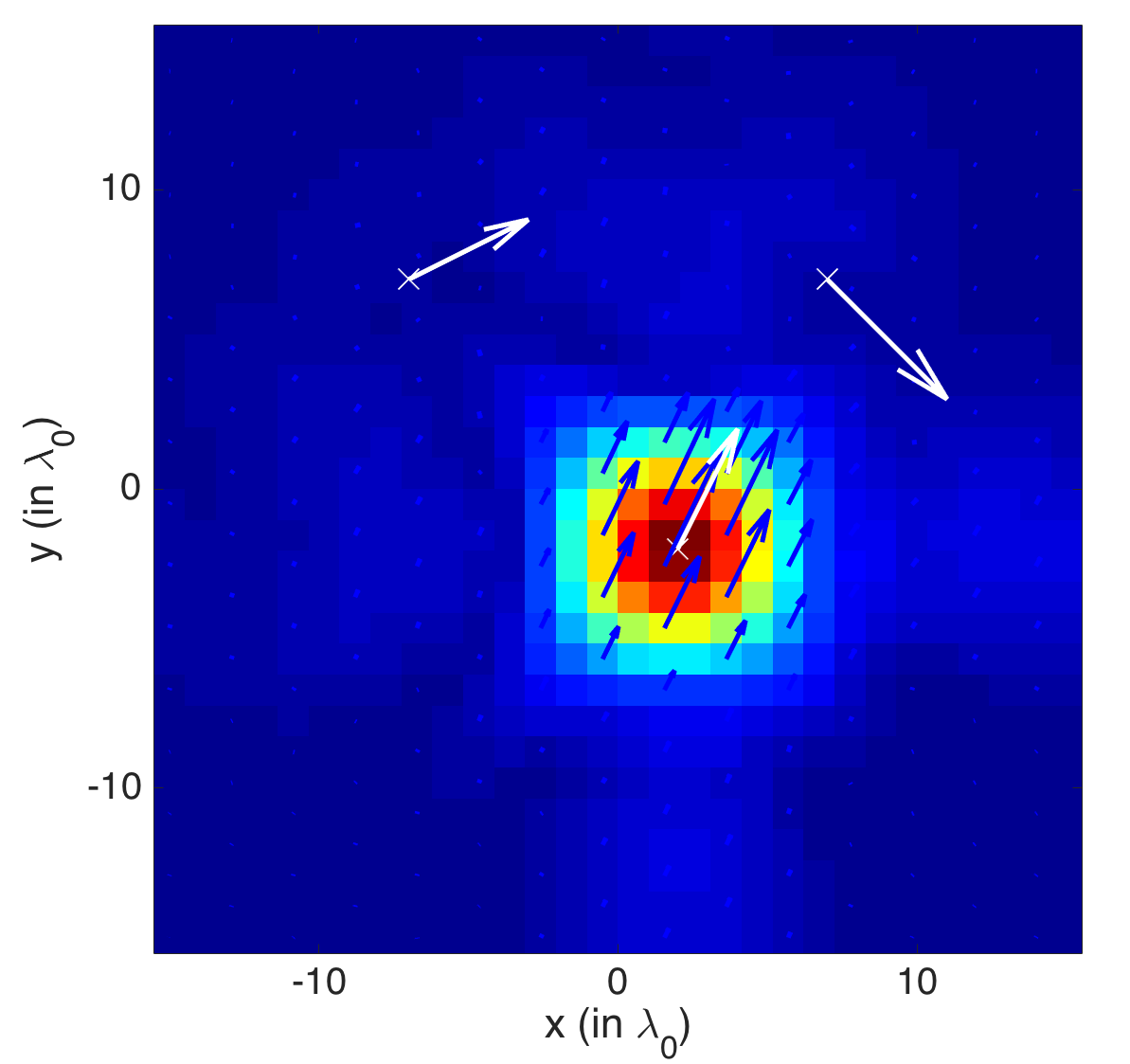 Figure 31
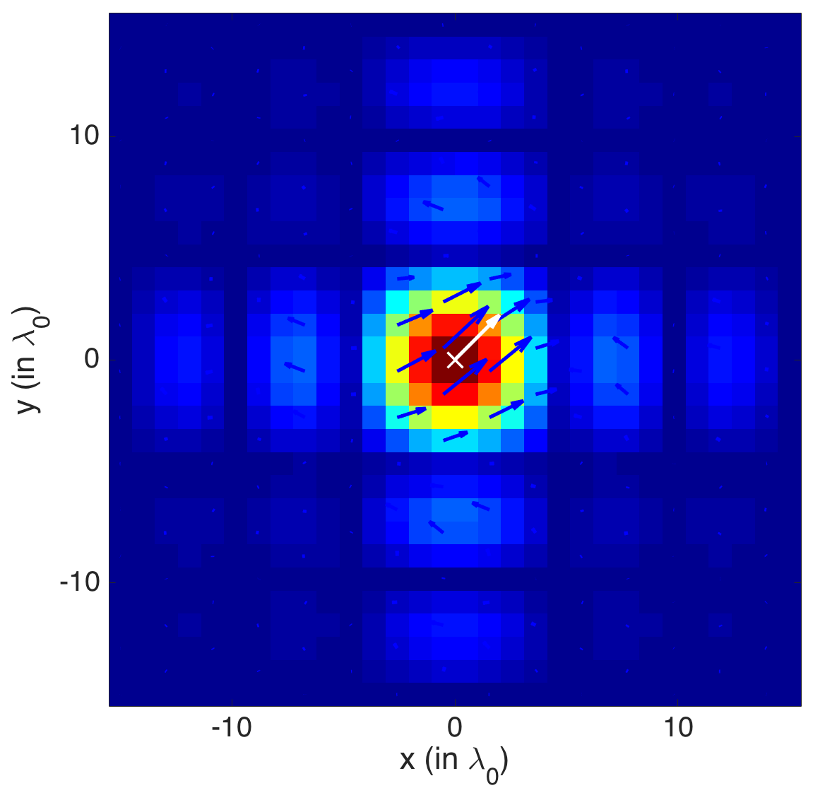 Figure 32
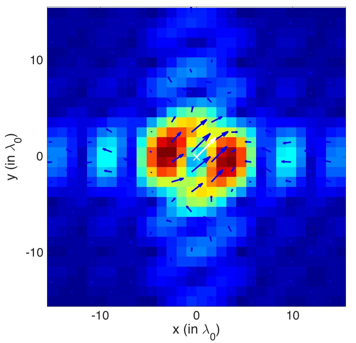 Figure 33
Peer Reviews
No public reviews on file for this paper yet. If you reviewed it on a platform where reviews are public (OpenReview, ICLR, NeurIPS, ICML), you can paste yours below so the community can read it here.
Videos
No videos yet. Explain this paper in a talk, walkthrough, or lecture? Add one.
Taxonomy
TopicsMicrowave Imaging and Scattering Analysis · Electromagnetic Scattering and Analysis · Numerical methods in inverse problems
Imaging polarizable dipoles
Maxence Cassier and Fernando Guevara Vasquez
Mathematics Department, University of Utah, Salt Lake City UT 84112
Mathematics Department, University of Utah, Salt Lake City UT 84112
Abstract.
We present a method for imaging the polarization vector of an electric dipole distribution in a homogeneous medium from measurements of the electric field made at a passive array. We study an electromagnetic version of Kirchhoff imaging and prove, in the Fraunhofer asymptotic regime, that range and cross-range resolution estimates are identical to those in acoustics. Our asymptotic analysis provides error estimates for the cross-range dipole orientation reconstruction and shows that the range component of the dipole orientation is lost in this regime. A naive generalization of the Kirchhoff imaging function is afflicted by oscillatory artifacts in range, that we characterize and correct. We also consider the active imaging problem which consists in imaging both the position and polarizability tensors of small scatterers in the medium using an array of collocated sources and receivers. As in the passive array case, we provide resolution estimates that are consistent with the acoustic case and give error estimates for the cross-range entries of the polarizability tensor. Our theoretical results are illustrated by numerical experiments.
Key words and phrases:
Kirchhoff migration, Maxwell equations, polarizability tensor, polarization vector
2000 Mathematics Subject Classification:
35R30, 78A46
Contents
-
2.3 The dyadic Green function in the Fraunhofer asymptotic regime
-
2.8.3 Numerical illustration of depth oscillation suppression
1. Introduction
The behavior of small scatterers in a homogeneous medium and subject to an electromagnetic field can be well described by a polarizability tensor (see e.g. [22]), which characterizes the effective response of the scatterer to the incident electric field. We present here an imaging method that produces tensor valued images of the polarizability tensor in a medium, by using measurements made at an array of collocated sources and receivers. This is active imaging because the array generates waves to probe the medium and could have applications to radar [15]. We also consider the passive imaging problem which consists in imaging the location and polarization vector of small electromagnetic sources within the medium, from measurements of their emitted electrical field on a (passive) array of receivers.
The imaging technique we use here is an analogue of Kirchhoff imaging (see e.g. [8]) in electromagnetics. This a well-understood technique in acoustics for both passive and active imaging. To our knowledge Kirchhoff imaging has not been thoroughly studied for electromagnetics. In acoustics, the Kirchhoff image resolution in a plane parallel to the array (i.e. the cross-range) is given by the Rayleigh criterion , where is the wavelength, is the distance between the array and the imaging plane and is array aperture (or diameter). The resolution in depth (in the range direction, perpendicular to the array) is governed by the frequency bandwidth of the measurements and is given by , where is wave velocity in the medium. For a mathematical derivation of these resolution results see e.g. [9].
One could view the active imaging problem we consider as an inverse medium problem. In the full aperture case (i.e. when the array completely surrounds the medium) the inverse medium problem is known to have a unique solution for the Maxwell equations [23, 16] and linearized approaches (i.e. based on the Born approximation) exist, see e.g. [17]. The passive problem for electromagnetics has been studied in [19]. To our knowledge, this work presents the first error estimates for reconstruction of polarization vectors (for the passive problem) and polarizability tensors (for the active problem).
Another way of approaching the active imaging problem for small inclusions is to study the behavior of the measurements as the size of the inclusions is driven to zero. This was done for the conductivity equation in [14] and was used to image small inhomogeneities in a known conductive medium in e.g. [14, 12]. It was demonstrated that information about the shape of the inclusions (namely an ellipsoid approximation) can be obtained with this method [14]. This asymptotic expansion has been carried out for other equations, e.g. for the Maxwell equations [26]. The asymptotic expansion can actually be carried further, revealing the so-called generalized polarizability tensors [1] which encode more information about the shape of the inclusions [2]. This approach has been applied to acoustics [5] and in the context of electromagnetism to detect small dielectric inhomogeneities characterized by a contrast in permittivity and permeability (see [4, 3, 26] for the asymptotic analysis and [6] for the imaging application). We emphasize that in our approach we are not after the geometric properties of each inclusion separately. We only seek the first polarization tensor (or matrix111Since all tensors we consider are matrices, we interchangeably use “tensor” and “matrix”.) at an imaging point, whether there is a scatterer or not, and study the resolution and accuracy of this image.
Our paper is organized as follows. The passive imaging problem is studied in section 2. The active case is considered in section 3. We conclude with a brief summary and future in section 4.
2. The passive imaging problem
It is convenient to use the dyadic Green function to represent Maxwell equation solutions, so we recall it in section 2.1. Then in section 2.2 we define the passive imaging problem and the data we use to image. Our analysis relies on the Fraunhofer asymptotic regime which is detailed in section 2.3. The generalization of the Kirchhoff imaging function to a vector valued image is explained in section 2.4. The remaining sections include the analysis of different aspects of this imaging function. The resolution estimate of the position in a plane parallel to the array (cross-range direction) is done in section 2.5. The extraction of the dipole polarization vector data from the vector valued Kirchhoff image is done in section 2.6. Section 2.7 includes the resolution of the position in the range direction, i.e. the direction perpendicular to the array, and section 2.8 studies the variation in range of the image and shows how to mitigate oscillations in range of the reconstructed polarization vector. We complement the theory with numerical experiments in section 2.9.
2.1. The dyadic Green function
We consider an electromagnetic homogeneous medium characterized by its dielectric permittivity and magnetic permeability which define its constant speed of propagation . We denote by the angular frequency and the wavenumber and by the matrix valued Green function associated with the time-harmonic Maxwell equations, i.e. the solution to
[TABLE]
where stands for the identity matrix, is the Dirac distribution at and for the curl operator of a matrix, defined as the curl of its three columns with respect to the variable. This so-called dyadic Green function , is given by (see e.g. [22])
[TABLE]
where , , and is the acoustic Green function in three dimensions
[TABLE]
The dyadic Green function is diagonalizable in an orthonormal basis because it is a normal matrix (i.e. commutes with ). Its eigenvalues are (with multiplicity 1 and corresponding eigenvector ) and (with multiplicity 2 and eigenspace being the orthogonal of ). We note that the largest eigenvalue in magnitude of is when , and thus the Green function becomes increasingly ill-conditioned as :
[TABLE]
2.2. Mathematical formulation of the passive imaging problem
We denote by the characteristic size of an array of collocated transmitters and receivers. For example a square array in the plane of side is given by . Note that we drop the arrow for two dimensional vectors, i.e. denotes the two first components of .
We consider a family of radiating electric dipoles located at with respective polarization vectors (also called dipole moments) (see figure 1).
The electric field (see [22]) emitted by this family of dipoles is a solution to the following time-harmonic equation on
[TABLE]
and thus can be expressed by virtue of (1) in terms of dyadic Green functions
[TABLE]
The passive imaging problem consists in finding the positions and polarizations of the electric dipoles from the data
[TABLE]
for , in other words full measurements of the electrical field on the array . This is the best case scenario, as it assumes we can measure all three components of the electric field at each point of the array.
2.3. The dyadic Green function in the Fraunhofer asymptotic
regime
Let and be respectively an imaging point and a receiver. The characteristic propagation distance here is . We assume that the scatterers lie in a known imaging window (see figure 2) of characteristic size in cross-range and in range, i.e. . We assume we are in the Fraunhofer asymptotic regime, i.e. that the following scalings hold (see e.g. [10, 11]).
- •
, (high frequency or large propagation distance)
- •
Fresnel number , i.e. small aperture: ,
- •
Fresnel number , i.e. small imaging window in cross-range:
- •
Fresnel number , i.e. small imaging window in range .
Moreover we assume that
[TABLE]
which amount to assume that the imaging window is small compared to the array aperture, i.e. .
We first approximate the acoustic Green function as in [10] by expanding the distance :
[TABLE]
since implies that .
Expanding the phase leads to
[TABLE]
since implies that and .
Using (4) and (5), we get the following expansion for the acoustic Green function
[TABLE]
where the Fraunhofer or paraxial approximation of the acoustic Green function is
[TABLE]
Using that , the dyadic Green function (2) becomes
[TABLE]
where we used the orthogonal projector defined by
[TABLE]
Finally, combining the relations (6) and (7), we obtain the asymptotic of the dyadic Green function in the Fraunhofer regime:
[TABLE]
2.4. The Kirchhoff imaging function in electromagnetics
In acoustics, the Kirchhoff imaging function is, up to conjugation, time reversing the data recorded at the array and propagating it to the medium [8, 9, 25]. For the Maxwell equations we consider the analogous imaging function
[TABLE]
In contrast with the acoustic case, the image we obtain is a vector field. Also the factor is there to offset a similar factor in the data (3) and simplifies our asymptotic analysis. The imaging function with data (3) is then
[TABLE]
where the matrix is
[TABLE]
The image at of a dipole located at with polarization is thus . The matrix is thus, in some sense, a matrix valued point spread function for the Kirchhoff imaging function.
To analyze the Fraunhofer asymptotics of (10), we introduce for and the matrix defined by
[TABLE]
Proposition 2.1**.**
The Kirchhoff imaging function (10) associated with data (3) is, in the Fraunhofer regime,
[TABLE]
Proof.
Using the asymptotic of the dyadic Green function (8), one can rewrite the matrices in the imaging function (10) as
[TABLE]
with a matrix whose asymptotic is given by:
[TABLE]
This last asymptotic follows from two facts. First the matrix norm of the orthogonal projectors and is uniformly bounded in (for any matrix norm choice). Second, the area of the array is . ∎
2.5. Cross-range estimation of positions
We start by analyzing the spatial resolution of the Kirchhoff imaging function (10). This is done by looking at the decay properties of the point spread function for away from a fixed dipole location . This decay comes from the (approximate) orthogonality of the acoustic Green functions and as functions of in and when and are “well separated”, see [9, 13, 25].
Since the imaging function is linear in the data we consider (without loss of generality) the case of a single obstacle located at . This is valid if we assume that the dipole polarizations have the same order of magnitude (i.e. ) and this implicitly assumed in the following. The resolution analysis in this section is done in the cross-range plane passing through the single obstacle. The range analysis is done later in section 2.7. The main result of this section is summarized by the following proposition.
Proposition 2.2** **(Imaging
function decrease in cross-range).
The Kirchhoff imaging function (10) of a dipole located at and evaluated at satisfies for with
[TABLE]
where the is explicitly given by . When the shape of the array is a disk of radius , one has
[TABLE]
Concretely, the asymptotics (15) and (16) in proposition 2.2 means that the image decays as we move away from the dipole location . The image is asymptotically zero compared to its value at , when is large with respect to . Hence the size of the focal spot in the cross-range is given by the Rayleigh resolution , as is the case in acoustics (see e.g. [8, 9]).
Remark 2.1**.**
In the particular case where the dipole polarization is aligned with the axis, the image at the dipole location is (see (16)). We estimated in (15) that the imaging function is small compared to for imaging points far way from the dipole location. Therefore it is not clear from this analysis if the image reveals the position of such a dipole. This case is considered later in section 2.7, when we consider multi-frequency images.
The proof of proposition 2.2 is a direct consequence of two results. The first one shows the decay of property of the image function using a stationary phase argument (lemma 2.1). The second one, explicitly calculates the value of the image at the dipole location using a circular array (lemma 2.2).
Lemma 2.1**.**
For , with , the matrix defined by (2.4) satisfies
[TABLE]
where the constant in the notation depends only on the shape of the array and the depth of the imaging window.
Proof.
To avoid writing a phase term many times, we introduce the matrix
[TABLE]
which satisfies . To prove (17), it is more convenient to use the rescaled array . By the change of variable , we can rewrite the matrix defined by (2.4) and (18) as
[TABLE]
where . Then, we follow the method proposed in [27], based on an integration by parts, to study the asymptotic of multivariate oscillating integrals. We denote by the scalar function:
[TABLE]
and by and the matrix-valued functions defined componentwise by
[TABLE]
for on the rescaled array . Using the identity:
[TABLE]
and the divergence theorem, we can rewrite the entries of as
[TABLE]
Replacing by its constant value , expressing the divergence of the second integral and then using the Cauchy-Schwarz inequality we obtain
[TABLE]
As the entries of an orthogonal projection are dominated by , we have
[TABLE]
which leads immediately to
[TABLE]
where is the perimeter of . A direct calculation gives
[TABLE]
for all points with . Applying this inequality and the fact that the entries of an orthogonal projector are bounded by we get
[TABLE]
This last inequality leads immediately to
[TABLE]
where is the area of . Finally, the asymptotic (17) for the matrix follows from the relations (20), (21), (22) and using the norm for the entries of a matrix. By equivalence of norms, it also holds for other matrix norms. ∎
We now continue with lemma 2.2 and study the asymptotics of . This is a special case because the integral (2.4) is not oscillatory, is independent of and simplifies to
[TABLE]
We compute explicitly this integral when the array is a disk, but this could be generalized to other simple geometries.
Lemma 2.2**.**
When the array is a disk of radius , we have the asymptotic
[TABLE]
For the proof of lemma 2.2, see appendix A.
Proof of proposition 2.2.
The proof is a direct consequence of proposition 2.1, lemmas 2.2 and 2.1 and the fact that the polarization vectors are assumed to have order one length. ∎
2.6. Cross-range estimation of the polarization vectors
We now extract from the Kirchhoff imaging function for dipoles (10) information about the polarization vectors . Assuming the dipole positions are known, the polarization vectors must satisfy
[TABLE]
If the dipoles are distant enough from each other, lemma 2.1 guarantees that the coupling terms remain small. Thus we estimate the by solving the linear system,
[TABLE]
Unfortunately, the systems (25) are ill-conditioned. Indeed, for a circular array of radius , the Fraunhofer asymptotic of the matrix (proposition 2.1 and lemma 2.2) gives
[TABLE]
Thus the matrix is asymptotically a singular matrix and one cannot expect retrieving the component of . The same asymptotic (2.6) reveals that the block of (corresponding to the two components of ) is invertible, with condition number close to .
We now derive an error estimate on . To this end we denote by the first two components of the imaging function and rewrite
[TABLE]
where , is the first principal submatrix of , etc
Proposition 2.3**.**
Let be a circular array of radius . In the Fraunhofer asymptotic regime, the system
[TABLE]
is invertible. The solution (which depends on the imaging point ) approximates the true cross-range polarization vector according to the following estimates
- •
If the imaging point coincides with a dipole, i.e. ,
[TABLE]
- •
If the imaging point does not coincide with a dipole in range, i.e. if for all ,
[TABLE]
Proof.
The asymptotic expansion (2.6) of yields immediately that for the induced matrix 2-norm,
[TABLE]
Hence, as soon as
[TABLE]
we have that the matrix is invertible. This is the case in the Fraunhofer regime because the left hand side of (31) is and one gets that is of order . Hence, in this regime, the system (28) admits a unique solution . When , we use the block decomposition (27) of and the identity (24) to get
[TABLE]
Using relations (32), (27) and (28) (which define the systems satisfied by and ) we get that:
[TABLE]
Finally, we apply lemma 2.1 and the asymptotic formulas (14) and (2.6) to dominate the right side of the last inequality:
[TABLE]
We now move to the case . From (28) we immediately get
[TABLE]
Then, using proposition 2.2 which expresses the decay of the Fraunhofer image in the case of one dipole and the linearity of with respect to the number of dipoles, we immediately get (30). ∎
The last proposition means that one obtains a good estimation of the two components of by solving the linear system (28) at . A part from terms that are small in the Fraunhofer regime, the error is due to the presence of the other dipoles and involves the cross-range distances . Thus the error in estimating the polarization vector is small when the dipoles are well separated, i.e. with distances large compared to the cross-range resolution . The asymptotic (30) tells us that is also a good imaging function for the dipole’s position since it decreases as reciprocal of the distance to the closest dipole. We expect to have the same resolution as the Fraunhofer imaging function (see proposition 2.2).
2.6.1. Numerical experiments
We illustrate our cross-range resolution analysis in figures 3 and 4. Our goal is to contrast the difference between solving for all 3 components of the polarization vector for a single dipole and solving only for the cross-range components. We consider a regime corresponding to microwaves in vacuum, i.e. propagation velocity m/s, frequency GHz and wavelength m. The array is a square centered at the origin and located within the plane . Its side aperture is and is composed of equally spaced, point-like receivers. The single dipole is located at and has polarization vector .
In figure 3, the reconstruction of both the position and polarization vector is performed by solving the ill-conditioned linear system (25). Here is a poor approximation to near the dipole location, so much so that the image appears as that of two nearby dipoles. Since the directions and are still well recovered, this means that is not well reconstructed. The focal spot is broader compared to that in figure 4, which indicates that does not give a precise reconstruction of the position. The recovery of the directions and is also worse than in figure 4 because they do not decrease as fast when one moves away from the dipole.
In figure 4, the reconstruction of both the position and cross-range polarization is performed by solving the well-conditioned linear system (25). At the dipole position we have , which is close to the true value and the focal spot is nicely centered about the dipole. The size of the focal spot is consistent with the Rayleigh criterion, i.e. . This confirms the asymptotic expression (30) which tells us that in the case of a single dipole, has a cross-range resolution similar to the Kirchhoff imaging function . Moreover, one gets a stable reconstruction of and near the dipole position.
2.7. Range estimation of the position
Similarly to the acoustic case, Kirchhoff migration can resolve the location of a reflector in depth (range) by integrating over a frequency band [8]. Here we consider the band with central frequency and bandwidth . By linearity, we consider only the case of a single dipole located at and polarization vector . For the analysis, we assume that the Fraunhofer asymptotic regime (see section 2.3) holds uniformly with in the whole frequency band . We study the following imaging function
[TABLE]
We suppose that the cross-range position of the obstacle is known and we evaluate the imaging function (33) at points of the form . Hence, using the asymptotic (13) of yields (for )
[TABLE]
The following proposition shows that as the range distance between the imaging point and the dipole is large compared to , the norm of the imaging function becomes small. This is similar to the range resolution estimate in acoustic [8, 9].
Proposition 2.4** (Imaging function decrease in the range direction).**
When the array is a disk of radius , the Kirchhoff imaging function (10) of the dipole satisfies for all with ,
[TABLE]
At the dipole location we have
[TABLE]
Proof.
When , we get
[TABLE]
for some , because orthogonal projectors have induced matrix 2-norm equal to one and the polarization vector is assumed to be . By evaluating the integral in frequency of the latter expression we obtain
[TABLE]
where . Hence we have that
[TABLE]
The expression (2.7) of the imaging function evaluated at the dipole location is
[TABLE]
and by lemma 2.2 satisfies the following asymptotic
[TABLE]
∎
2.8. Polarization vector recovery in the range direction
As we discussed in section 2.6, we cannot expect to stably recover the range component of a dipole’s polarization vector from the Kirchhoff image . A straightforward integration in frequency of the linear system approach of section 2.6 gives a good estimate of the cross-range polarization vector if we knew the range position of the dipole. Unfortunately, moving in depth gives oscillatory artifacts in . We characterize these artifacts and show how to eliminate them.
2.8.1. Analysis of polarization vector image in range
For the analysis, we consider once again a family of dipoles with positions and polarizations . To recover the cross-range components of the polarization vectors, we integrate (28) over the frequency band and solve the following linear system
[TABLE]
where denotes the two first components of the imaging function . Naturally, the solution of this system leads to a stable reconstruction of both the position and the polarization of each dipole in the cross-range. Indeed, it is straightforward to check that integrating the system (28) over the frequency band does not change: (a) its invertibility in the Fraunhofer regime, (b) its condition number being close to one and (c) the resolution estimates (29) and (30).
Now we study the behavior in range of this procedure to recover the cross-range component of the polarization vector image . Here we isolate the effect of range by considering the case where all the dipoles have same cross-range, i.e. for . The following proposition shows that the resolution of in the range direction is (as in acoustics, see e.g. [8, 9]). Furthermore at the dipole position , one recovers the polarization vector provided that the range distance between the different dipoles is large with respect to the range resolution .
Proposition 2.5**.**
When the array is a disk of radius and the dipoles are all aligned in the range direction of , the cross-range polarization image (obtained by solving the linear system (38) and depending of the imaging point ) satisfies the two following estimates:
- •
If the imaging point is the dipole location, i.e. we have
[TABLE]
- •
If the imaging point range is different from any of the dipole ranges, (for all ),
[TABLE]
Proof.
We introduce for convenience the matrix
[TABLE]
When , the cross-range component of the polarization satisfies
[TABLE]
which is the integral over the frequency band of (32). Thus from the systems (41) and (38) satisfied by and one gets
[TABLE]
By proceeding as in the proof of proposition 2.3, one can show by integrating over the frequency band that . Since the dipoles are aligned, the contribution from the other dipoles can be controlled using proposition 2.4, giving
[TABLE]
Moreover, the asymptotic (2.6) bounds the error due to only looking at the cross-range component of the system: . Combining the last three estimates gives the desired result (39).
Finally, the asymptotics (40) follows immediately from and the decay rate in range of the imaging function (35). ∎
2.8.2. Depth oscillation artifact and its suppression
It is known in acoustics that the reflection coefficient of a point scatterer can only be recovered up to a complex phase, see e.g. [21]. A similar phenomenon is observed here: if the range position of a scatterer is not known perfectly, the estimation of the cross-range polarization oscillates in range. This can be easily seen by considering a single dipole at location and with polarization vector . Rewriting the imaging function for points with same cross-range as the dipole gives together with (2.7) and (37)
[TABLE]
Clearly the presence of the complex exponential and the causes the image to oscillate in . This oscillation is not taken into account if we solve the linear system (38) for , indeed the system matrix does not oscillate but the right hand side does. We point out that in the case , there are no such oscillations, which explains why this error is not present in the error analysis for assuming a known dipole position (39). Also the oscillations are relevant because their length scale is close to , the resolution in depth.
To deal with this artifact, we estimate by solving (38) and then we fix the phase of one component of . In the following, we have arbitrarily chosen to enforce that the first component be real and positive, that is . This can be achieved by post-processing the solution of (38) by the operation . This operation is problematic for small , in which case we can use the component or we could also regularize using: , for a small .
2.8.3. Numerical illustration of depth oscillation suppression
Here we illustrate the depth oscillation and its correction in the same setup as that in figures 3 and 4. In figure 5 we display in color scale and with arrows the plane . The central frequency is and the bandwidth are both equal to GHz. Thus, the ratio gives in both images the size of the focal spot in the range direction . On the left, we display without any phase correction. The dipole position and magnitude are accurately imaged, but the dipole polarization vector oscillates in range direction inside the focal spot with a period . Hence the reconstruction is unstable. In the right figure, we apply the correction to both the reconstructed and the true (white arrows). The correction suppresses the phase oscillation and gives a stable reconstruction of , up to a complex sign.
2.9. Numerical experiments for several dipoles
In figures 6, 7 and 8, we consider the case of three dipoles placed at , and with respective polarization vectors , , and . The cross-range polarization vector components have norms , and , respectively. The array , the bandwidth and the central frequency are identical to the ones used in figure 5. We visualize with the same convention as in the previous figures the reconstruction of the positions and the polarization vectors obtained by solving the linear system (38) and applying the phase correction of section 2.8.2. Figures 6 and 7 illustrate the reconstruction and the resolution of in the cross-range of each dipole. Once again, the focal spot is given by the Rayleigh criterion: . In each case, we observe a stable reconstruction of and of the complex vector . Figure 8 illustrates the range resolution of each dipole. The size of the focal spot is again of order . We note a stable reconstruction of with no oscillations in the range direction (as by convention , it is not represented in our figures). Even if is reconstructed accurately by our method, we chose not to display it in figure 8 because the axis are .
3. The active imaging problem
Here we focus on the imaging problem where the array is composed of sources and receivers. The problem and the imaging function we use are defined in section 3.1. The generalization of the Kirchhoff imaging function we consider associates to each imaging point a matrix. As we show in section 3.2, the cross-range resolution estimate for the norm of this matrix coincides with the classic estimate in acoustics. The procedure to extract the polarizability tensor from the image is given in section 3.3. We then proceed to study the resolution in the range direction and we obtain results that are similar to those in acoustics (section 3.4). The reconstructed polarizability in range is studied in section 3.5. As in the passive case, the image needs to be corrected in the depth direction to suppress oscillatory artifacts. Finally we report numerical experiments illustrating our results in section 3.6.
3.1. Mathematical formulation of the active imaging problem
We now consider the problem of imaging point-like scatterers using a collocated array of sources and receivers within the plane (see figure 9). The field scattered by a small object located at resulting from an incident field is
[TABLE]
where is the polarizability tensor of the scatterer, satisfying by reciprocity, see e.g. [22]. The analogue in acoustics of the matrix is the reflection coefficient. In general, the polarizability tensor depends on , but for our study we assume that the dependence is weak within the frequency band we consider (this occurs when e.g. the scatterers are standard dielectric, [20]). Our goal is to image both the position and polarizability tensors of a collection of these scatterers. We work under a weak scattering assumption, where the scattered field from scatterers located at with polarizability tensors , is given by the Born approximation (see e.g. [11])
[TABLE]
The field used to probe the medium is controlled by a distribution where is the polarization vector of a dipole at . The electric field generated by the array dipole distribution is
[TABLE]
The data we use to image is the scattered field at the array. Since different array dipole distributions can be used, the data that can be collected in this setup can be thought of as the (matrix valued) array response function defined for and wavenumber such that the scattered field resulting from the array dipole distribution is
[TABLE]
Combining (43) and (44), the array response function for point-like scatterers is
[TABLE]
The imaging function we use is an electromagnetic version of the Kirchhoff imaging function
[TABLE]
which gives a complex matrix at each imaging point . For our particular data, the image is
[TABLE]
where the matrix is the “point spread matrix” defined in (11).
3.2. Cross-range estimations of the position
To estimate the cross-range resolution of the active Kirchhoff imaging function , we consider the case of one point-like scatterer () located at with polarizability tensor . We assume that the range position is known. The case of multiple point-like scatterers is obtained by linearity. In the following we assume that . It is convenient to introduce the block decomposition of the polarizability tensor
[TABLE]
where , is a matrix, is a matrix, and so on.
The next proposition shows that the cross-range resolution of the Kirchhoff imaging function is also given by the Rayleigh criterion . The difference from imaging active sources is that for scatterers, the image function decays faster. To be more precise, the decay is in the order of for scatterers versus for sources, see proposition 2.2.
Proposition 3.1** (Decreasing of the imaging function in cross-range).**
The Kirchhoff imaging function (47) of a point-like scatterer located at and evaluated at satisfies
[TABLE]
where the is explicitly given by . When the shape of the array is a disk of radius , one has
[TABLE]
Proof.
Let be a point in the cross-range of the dipole with . As and , one gets immediately from the expression (47) of (with ) that
[TABLE]
Using proposition 2.1, it is straightforward to derive the following Fraunhofer asymptotic for the matrix
[TABLE]
which leads to (48) by applying lemma 2.1 for the asymptotic of the matrix .
For the case of a disk array of radius , the asymptotic formula (49) of follows immediately from the asymptotic (50) when and the lemma 2.2 for the asymptotic of the matrix . ∎
3.3. Cross-range estimations of the polarizability tensors
We now study the estimation of the polarizability tensors of point-like scatterers from the Kirchhoff imaging function. We derive an error estimate by assuming that the positions of the point-like scatterers are known. At we have the following identity
[TABLE]
where we use that , from (11) and the fact that and commute. Hence, if the point-like scatterers are distant enough, we expect the coupling term (i.e. the second term in the right hand side of (51)) to be small. Neglecting the coupling terms, can be obtained by solving the linear system
[TABLE]
In the Fraunhofer regime, this system is ill-conditioned. Indeed, from formula (2.6), it follows that the matrix is ill-conditioned. Hence, as for the passive imaging problem, one cannot retrieve all entries of the polarizability tensor . To be more precise, the asymptotic formula (2.6) shows that in this regime the blocks , and are asymptotically smaller compared to the block . The block can be approximated by , where is the identity. Hence we can stably extract from (51) the block of the polarization tensor. We give an error estimate for this procedure in the following proposition.
Proposition 3.2**.**
In the Fraunhofer asymptotic regime, the system
[TABLE]
is invertible and its solution is
[TABLE]
If the array is a disk of radius , the estimated cross-range polarizability tensor (which depends on the imaging point ) approximates the exact one in the following sense
- •
If the imaging point coincides with a dipole, i.e. ,
[TABLE]
- •
If the imaging point does not coincide with a dipole in the range, i.e. for all ,
[TABLE]
Proof.
For simplicity we omit the dependence in in this proof. In Fraunhofer asymptotic regime, is invertible with (see proposition 2.3). Thus the solution of (53) is given by formula (54).
In the case , the identity (51) and the asymptotic (2.6) of the matrix , gives after a short calculation that the first block of the exact polarizability tensor satisfies the following system
[TABLE]
We deduce that the difference between the estimated (satisfying (53)) and the true (satisfying (3.3)) is
[TABLE]
Finally, using the asymptotic formula (48) to control the terms in sum above we obtain
[TABLE]
In the case , we have
[TABLE]
Thus, the asymptotic formula (56) follows immediately from the decay of the imaging function given by (48). ∎
The asymptotic (55) shows that one obtains a good reconstruction of the cross-range polarizability tensor by solving the linear system (53). The error is given by a coupling term (contribution from the other scatterers) and remainders which are small in the Fraunhofer regime. This coupling term decreases as which is faster than the decrease in we found in passive imaging (see proposition 2.3). The asymptotic (56) shows that using as an image (as it does depend on the imaging point ) also leads to a stable reconstruction of the scatterer’s positions, with cross-range resolution given by the Rayleigh criterion.
3.4. Range estimation of the position
We study the resolution in range by considering one point-like scatterer located at with known cross-range position . We assume the array response function is known for and on the frequency band , with bandwidth . The Kirchhoff imaging function over this band and at a point is obtained from the single frequency Kirchhoff imaging function (46) by integrating over the frequency band
[TABLE]
As in the passive case, we assume that the Fraunhofer asymptotics (section 2.3) hold uniformly over the frequency band . The next proposition shows that as in the passive imaging case, the range resolution is .
Proposition 3.3** (Imaging function decrease in the range direction).**
When the array is a disk of radius , the Kirchhoff imaging function (10) of the dipole satisfies for all with ,
[TABLE]
At the dipole location we have
[TABLE]
Proof.
We first consider the case where the imaging point does not coincide with the dipole, i.e. . Using the asymptotic (14) and the definition of in (2.4), we observe that the imaging function (47) at is
[TABLE]
where we used the notation
[TABLE]
Integrating in frequency we get
[TABLE]
Finally combining this last relation with (60) yields
[TABLE]
The asymptotic formula (58) follows.
When , the asymptotic formula (59) follows immediately by integrating over the frequency the asymptotic (49). ∎
3.5. Polarizability tensor recovery in the range direction
From the asymptotic analysis of section 3.2, at a frequency we can only expect to recover the cross-range polarizability tensor by solving the linear system (54). The solution depends on both the imaging point and the frequency . Since we assume that the true polarizability tensor does not depend on we propose to estimate it by averaging the single frequency estimate over the frequency band, i.e.
[TABLE]
As we see next in section 3.5.1, if the depth of the scatterer is well-known, this procedure estimates well the cross-range polarizability of the scatterer. However, as in the passive case (see section 2.8), the image oscillates in depth. These oscillations can be characterized and suppressed as we show in section 3.5.2.
3.5.1. Analysis of polarizability tensor image in range
In the next proposition, we isolate the effect of depth by considering scatterers that are aligned in range. We show that the depth resolution of the cross-range polarizability tensor image is , i.e. identical to the passive case (section 2.7). If the imaging point coincides with the scatterer position, the error in estimating the cross-range polarizability tensor remains small, provided the scatterers are well separated, i.e. is large with respect to the range resolution .
Proposition 3.4**.**
When the array is a disk of radius and the dipoles are all aligned the range direction of , the image of the cross-range polarizability tensor (given by (63)) satisfies the two following estimates:
- •
If the imaging point is the dipole location, i.e. , we have
[TABLE]
- •
If the imaging point range is different from any of the dipole ranges, (for all ),
[TABLE]
Proof.
We start with the case where . To shorten notation we use instead of . From the definition of the cross-range polarizability tensor image (63) and our assumption that the exact cross-range polarizability is independent of frequency we get
[TABLE]
To estimate the difference we use (53) and (3.3) to obtain
[TABLE]
Now recalling that , one gets that
[TABLE]
Then, since the dipoles are aligned, one can use the relation (62) to rewrite the coupling term in terms of a to get
[TABLE]
This gives the asymptotic (64). The asymptotic (65) can be proved in a similar way. ∎
3.5.2. Suppression of oscillatory artifact in depth
The image of the cross-range polarizability oscillates depth. To see this, consider the reconstruction formula (63) for a single dipole () located at and with polarizability tensor for imaging points in the range of the dipole . The multi-frequency estimate of the cross-range polarizability tensor is
[TABLE]
Using the asymptotic and the asymptotic (60) and (61) for in the range direction of , this becomes:
[TABLE]
for . The presence of the complex exponential and the causes the image to oscillate in (twice faster than in passive imaging see (42)). Thus, if one does not know exactly the cross-range position of the dipole, one cannot reconstruct in a stable way . To deal with this artifact, we fix the phase of one component of . In the following, we have arbitrarily chosen to enforce that the entry be real and positive, i.e. . This can be achieved by post-processing the solution of (38) by the operation . If is small, this operation can be problematic and we can instead fix the phase of another entry of . One can also regularize using , for a small .
3.6. Numerical experiments
3.6.1. Experiments without noise
Figures 10, 11, 12 and 13 illustrate the case of three point-like scatterers in a configuration identical to that in figures 6, 7 and 8. The dipoles are located at , and . Their polarizability tensors are symmetric complex matrices, with entries given in appendix B. We use the reconstruction formula (63) to recover the block of each dipole. The Frobenius norms of the cross-range polarization tensors are approximately 3.9, 3.5 and 4.5, respectively.
In figures 10 and 11, we visualize in the cross-range (figure 10) and range (figure 11) of the different dipoles. We use ellipses to visualize the real symmetric matrices and . The principal axis of the ellipses represent the orientation and magnitude of the matrices. The ellipses are plotted at the scatterer cross-range positions (figure 10) and range positions (figure 11). The white and yellow ellipses represent respectively the real part and imaginary part of the exact cross-range polarizability tensors. The dashed black and purple ellipses are those associated with the reconstructed quantities (real and imaginary, respectively).
We observe that the Frobenius norm is well estimated for all dipoles in both range and cross-range. The focal spot is consistent with the Rayleigh criterion in the cross-range (figure 10) and with in the range (figure 11). Furthermore, in figure 10, the image decays away from the scatterer positions faster than in passive imaging (see figures 6, 7 and 8) which confirms the asymptotics (29) and (56). Finally the matrices and are well reconstructed at the scatterer positions. Their corresponding ellipses agree in both range and cross-range.
To show the stability of the reconstructions in the focal spot we display in figures 12 and 13 the corresponding ellipses at locations (in range and cross-range) around the focal spot of one particular dipole. These images (and figures 14, 15 and 17) were obtained with a modified version of the plot_tensor_field function in [24]. We emphasize that the image in range (figure 13) is stable in depth because we used the correction explained in section 3.5.2. In figures 12 and 13, we use ellipses to visualize the matrices (left) and (right) in the vicinity of the cross-range (figure 12) and range position (figure 13) of the dipole located at . The color of the ellipses is proportional to the Frobenius norm of . Comparing these ellipses to the exact ones of figures 10 and 11 confirms that the correction suppresses the oscillation in depth and gives a stable reconstruction of , up to a complex sign.
3.6.2. Experiments with noise
For this experiment, the array is a square containing collocated sources and receivers and that we have equally spaced frequency samples in the band . To simulate noise in the measurements, we add a matrix with zero mean uncorrelated Gaussian distributed entries to the data defined in (45), where . The matrices for each frequency are uncorrelated. As in [10], we choose to fix the level of noise with respect to the average power received by the array of the signal on frequency band, namely:
[TABLE]
where stands for the Frobenius norm. The expected noise power is given by
[TABLE]
The signal-to-noise ratio (SNR) in decibels (dB) is then
[TABLE]
Figures 14 and 15 reproduce the numerical experiments of figures 12 and 13 but with a SNR of dB (i.e. the noise power is 10 times larger than the signal power). With noise present, the ellipse orientations agree with the true ones at the focal spot, but are significantly different away from the focal spot, where the image magnitude is also small. We conclude that Kirchhoff imaging is robust to relatively large measurement noise (as in acoustics, see e.g. [10]).
3.6.3. Experiments with an extended dipole distribution
In the figures 16, 17 and 18 we deal with the case of a volumetric polarizability tensor distribution within a cube of side , with center . This distribution is uniform and generated by a set of dipoles separated by a wavelength of . All the dipoles are assumed to have the same complex symmetric polarizability tensor
[TABLE]
The array , the central frequency and the frequency band are identical to the ones of figure 5.
In figure 16 (left), we observe a good reconstruction of the location of the scatterer in the cross-range plane . The right figure shows that only the edges of the cube are imaged in the range direction. Thus the Kirchhoff imaging function detects only the discontinuities of an extended scattered (as in acoustics [8]). In contrast to point-like scatterers, the information about the norm is lost here but one still observes a very good estimation of the orientations after normalization and up to a complex sign. The quality of the reconstruction can also be seen in figures 17 and 18 which shows the reconstructed tensors are stable in the vicinity of the scatterer in cross-range (figure 17) and range (figure 18).
4. Summary and future work
We used the Fraunhofer asymptotic to study an electromagnetic version of the Kirchhoff imaging function for both the passive and active imaging problems. The images we obtain are vector (resp. matrix) valued in the passive (resp. active case). The norm of these images behaves like the images in acoustics, meaning that we get identical resolution estimates for the position of well-separated dipoles (or scatterers) as those we would obtain in acoustics. The vector (or matrix) valued image contains information about the polarization vector (or polarizability tensor) of the point sources (or small scatterers) in the medium. We show how to extract this information to stably image these quantities. Our asymptotic reveals that we can only expect to stably recover the cross-range components of these quantities. The range components are lost.
This is a first step to understand what quantities can be imaged in an idealized case. Indeed, the data we used may be complicated to acquire in practice, as we need to measure at least the two cross-range components of the electric field in the passive case. In the active case we also need experiments where one can control the cross-range polarization vector components of the array sources.
We are currently adapting this imaging technique to a case where only cross-correlations of the electric field are available at the array, i.e. we assume we can only measure the electric coherence matrix
[TABLE]
for all points in the array. Here represents averaging over realizations of the electromagnetic field (which is assumed stationary so there is no dependence on ). This data is equivalent to knowing the Stokes parameters (see e.g. [18]), which characterize the polarization of electromagnetic waves. The technique we plan to use is a generalization of the imaging with cross-correlations method for acoustics in [7] to the Maxwell equations.
Appendix A Proof of lemma 2.2
Proof.
We consider a point with . In cylindrical coordinates the array is given by
[TABLE]
Thus, it leads to the following expression of in cylindrical coordinates:
[TABLE]
with
[TABLE]
Integrating in and using the Fraunhofer asymptotic to simplify the resulting expression and finally integrating in leads to
[TABLE]
The formula (23) follows by combining (66), (LABEL:eq.projpolar) and using the relation: . ∎
Appendix B Polarizability tensors used in numerical experiments
In section 3.6, the polarizability tensors that we used are the complex symmetric matrices given by
[TABLE]
Acknowledgements
The work of M. Cassier and F. Guevara Vasquez was partially supported by the National Science Foundation grant DMS-1411577. FGV would like to thank Arnold D. Kim for inspiring conversations about this problem.
The reference list from the paper itself. Each links out to its DOI / PubMed record.
- 1Ammari and Kang [2003] H. Ammari and H. Kang. Properties of the generalized polarization tensors. Multiscale Modeling and Simulation , 1(2):335–348, 2003. doi: 10.1137/S 1540345902404551 .
- 2Ammari and Kang [2007] H. Ammari and H. Kang. Polarization and moment tensors , volume 162 of Applied Mathematical Sciences . Springer, New York, 2007. ISBN 978-0-387-71565-0. doi: 10.1007/978-0-387-71566-7 . With applications to inverse problems and effective medium theory.
- 3Ammari and Khelifi [2003] H. Ammari and A. Khelifi. Electromagnetic scattering by small dielectric inhomogeneities. Journal de mathématiques pures et appliquées , 82(7):749–842, 2003. doi: 10.1016/S 0021-7824(03)00033-3 .
- 4Ammari et al. [2001] H. Ammari, M. S. Vogelius, and D. Volkov. Asymptotic formulas for perturbations in the electromagnetic fields due to the presence of inhomogeneities of small diameter II. The full Maxwell equations. Journal de mathématiques pures et appliquées , 80(8):769–814, 2001. doi: 10.1016/S 0021-7824(01)01217-X .
- 5Ammari et al. [2013] H. Ammari, J. Garnier, W. Jing, H. Kang, M. Lim, K. Sø lna, and H. Wang. Mathematical and statistical methods for multistatic imaging , volume 2098 of Lecture Notes in Mathematics . Springer, Cham, 2013. ISBN 978-3-319-02584-1; 978-3-319-02585-8. doi: 10.1007/978-3-319-02585-8 .
- 6Ammari et al. [2014] H. Ammari, J. Chen, Z. Chen, J. Garnier, and D. Volkov. Target detection and characterization from electromagnetic induction data. Journal de mathématiques pures et appliquées , 101(1):54–75, 2014. doi: 10.1016/j.matpur.2013.05.002 .
- 7Bardsley and Guevara Vasquez [2016] P. Bardsley and F. Guevara Vasquez. Kirchhoff migration without phases. Inverse Problems , 32(10):105006, 2016. doi: 10.1088/0266-5611/32/10/105006 .
- 8Bleistein et al. [2001] N. Bleistein, J. K. Cohen, and J. W. Stockwell, Jr. Mathematics of multidimensional seismic imaging, migration, and inversion , volume 13 of Interdisciplinary Applied Mathematics . Springer-Verlag, New York, 2001. ISBN 0-387-95061-3. doi: 10.1007/978-1-4613-0001-4 . Geophysics and Planetary Sciences.