An upper bound for the KS-entropy in quantum mixing systems
Ignacio S. Gomez

TL;DR
This paper derives an upper bound for the Kolmogorov-Sinai entropy in quantum mixing systems using quantum phase space graininess, a rescaled entropy, and correlation properties, linking classical and quantum chaos features.
Contribution
It introduces a novel method to estimate the KS-entropy upper bound in quantum systems considering quantum phase space graininess and mixing correlations.
Findings
Derived an upper bound for quantum KS-entropy.
Linked quantum mixing properties with classical ergodic hierarchy.
Identified the quantum logarithmic timescale in chaotic systems.
Abstract
We present an upper bound for the Kolmogorov-Sinai entropy of quantum systems having a mixing quantum phase space. The method for this estimation is based on the following ingredients: i) the graininess of quantum phase space in virtue of the Uncertainty Principle, ii) a time rescaled KS-entropy that introduces the characteristic timescale as a parameter, and iii) the factorization property of the mixing correlations. The analogy between the structures of the mixing level of the ergodic hierarchy and of its quantum counterpart is shown. Moreover, the logarithmic timescale, characteristic of quantum chaotic systems, is obtained.
Click any figure to enlarge with its caption.
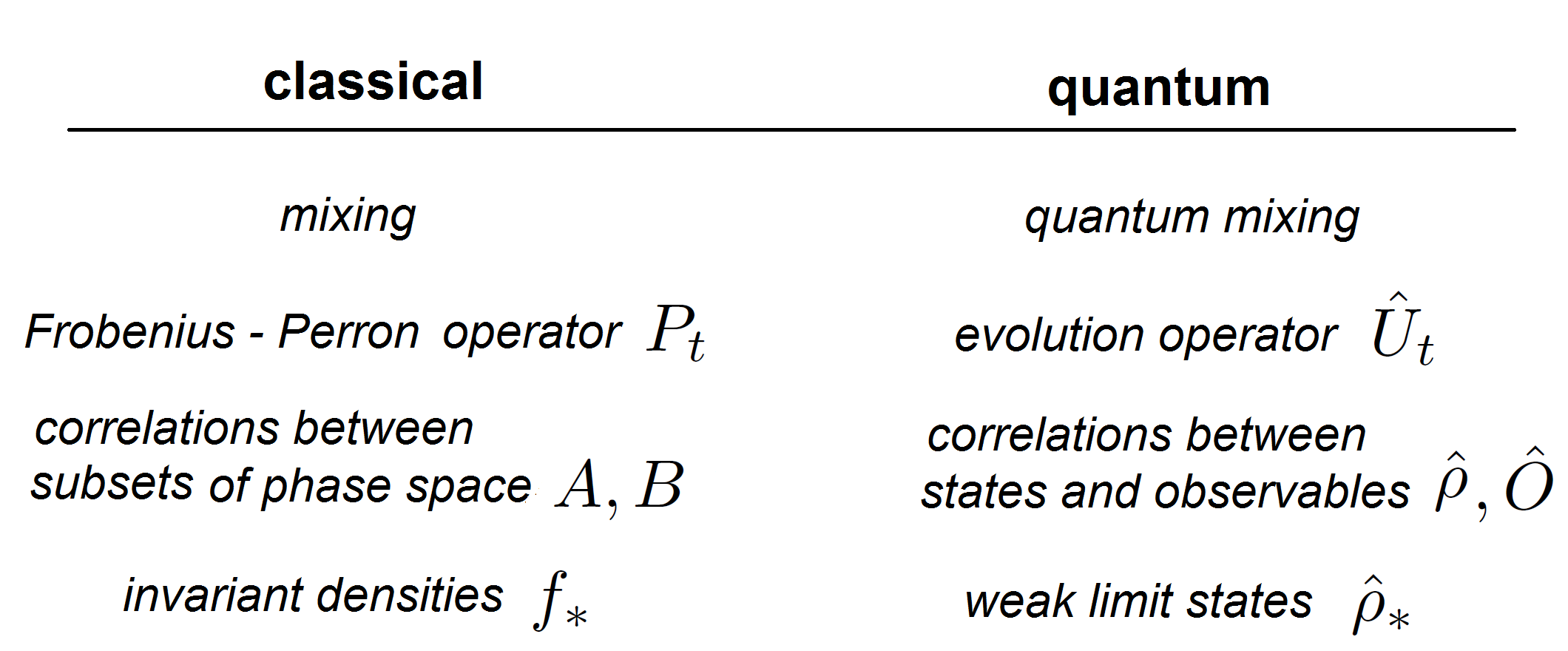 Figure 1
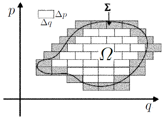 Figure 2
Peer Reviews
No public reviews on file for this paper yet. If you reviewed it on a platform where reviews are public (OpenReview, ICLR, NeurIPS, ICML), you can paste yours below so the community can read it here.
Videos
No videos yet. Explain this paper in a talk, walkthrough, or lecture? Add one.
Taxonomy
TopicsQuantum chaos and dynamical systems · Quantum Mechanics and Applications · Chaos control and synchronization
An upper bound for the KS–entropy in quantum mixing systems
Ignacio S. Gomez
Abstract
We present an upper bound for the Kolmogorov–Sinai entropy of quantum systems having a mixing quantum phase space. The method for this estimation is based on the following ingredients: i) the graininess of quantum phase space in virtue of the Uncertainty Principle, ii) a time rescaled KS–entropy that introduces the characteristic timescale as a parameter, and iii) the factorization property of the mixing correlations. The analogy between the structures of the mixing level of the ergodic hierarchy and of its quantum counterpart is shown. Moreover, the logarithmic timescale, characteristic of quantum chaotic systems, is obtained.
IFLP, UNLP, CONICET, Facultad de Ciencias Exactas, Calle 115 y 49, 1900 La Plata, Argentina
Keywords: KS–entropy – Mixing – Graininess – Logarithmic timescale
1 Introduction
Kolmogorov–Sinai entropy (KS–entropy) is considered as one of the most robust and significant indicator of chaos, theoretically and for applications [1, 2, 3, 4]. Basically, the KS-entropy assigns measures to bunches of trajectories and computes the Shannon-entropy per time-step of the ensemble of bunches in the limit of infinitely many time-steps. Moreover, the Pesin theorem [5, 6] links the KS-entropy with the Lyapunov coefficients which are a measure of the exponential instability, i.e. they characterize the chaotic motion. In turn, in classical mechanics the two properties necessary for chaos to occur are a continuous spectrum and a continuous phase space [7].
However, in quantum mechanics the arising of chaos is more subtle. Firstly, the most of quantum systems which present chaotic features in its classical limit have discrete spectrum and secondly, the Correspondence Principle CP implies the transition from quantum to classical mechanics for all phenomena including the chaos. Furthermore, by the Uncertainty Principle the quantum phase space is discrete and divided into elementary cell of finite size, which constitutes the so called graininess. Despite these difficulties, the KS–entropy allows one to give a concrete answer about the emergence of chaos in the classical limit, i.e. the quantum chaos [8, 9, 10]. The key point is that one can model the behavior of classical chaotic systems of continuous spectrum from classical discretized models in such way that the KS–entropies of the continuous and the discrete one tend to coincide for a certain appropriate range [11, 12, 13, 14, 15, 16]. This remark is crucial in order to obtain the characteristic timescales of quantum chaos where the classically behavior and the chaotic one overlap each other [17].
On the other hand, many chaotic systems of interest are mixing, i.e. the subsets of phase space have a correlation decay such that any two subsets are statistically independent for large times [2, 18, 19, 20]. This property is one of the most useful concepts to describe phenomena such as chaos, approach to equilibrium and relaxation in dynamical systems theory [7]. In a series of works quantum extensions of the mixing property were proposed [21, 22, 23, 24, 25, 26], from which we characterized the chaotic behaviors of the Casati–Prosen model [22, 27] and the kicked rotator [9, 10, 22], and recently the Gaussian Orthogonal Ensembles were obtained [26].
The main goal of this paper is to obtain an expression of the KS–entropy for quantum systems having a mixing classical analogue, making use of the quantum phase space graininess and the mixing property. Moreover, our approach allows one to shed light on the foundations of the quantum chaos. In particular, we obtain the logarithmic timescale as a consequence of the formalism presented.
The paper is organized as follows. In Section 2 we give the preliminaries that we employ throughout the paper. In Section 3 we prove some properties of the mixing correlations which are the key to obtain the KS–entropy. In Section 4 we give an upper bound of the KS–entropy obtained by means of the discretized quantum phase space and the time–rescaling property of the KS–entropy. Here we obtain the logarithmic timescale as a consequence of the estimation of the KS-entropy. Finally, in Section 5 we discuss and draw some conclusions.
2 Preliminaries
We give the notions and concepts to develop the results of the paper. First of all, we clarify the notation we will use throughout the paper.
We denote by the mean value of observable when the system is in state , i.e. where is the trace operator. If is any initial state at time , we denote by the state at time , i.e. where is the well-known operator evolution for Hamiltonian , and is its adjoint operator.
2.1 Kolmogorov–Sinai entropy
We recall the definition of the KS–entropy within the standard framework of measure theory [2, 18, 20]. Consider a dynamical system given by , where is the phase space, is a -algebra, is a normalized measure and is a semigroup of preserving measure transformations. For instance, could be the classical Liouville transformation or the corresponding classical transformation associated to the quantum Schrödinger transformation. is usually for continuous dynamical systems and for discrete ones.
Let us divide the phase space in a partition of small cells of measure . The entropy of is defined as
[TABLE]
Now, given two partitions and we can obtain the partition which is , i.e. is a refinement of and . In particular, from we can obtain the partition being the inverse of (i.e. ) and . From this, the KS–entropy of the dynamical system is defined as
[TABLE]
where the supreme is taken over all measurable initial partitions of . From the viewpoint of information theory, the Brudno theorem says that the KS–entropy is the average unpredictability of information of all possible trajectories in the phase space. Furthermore, Pesin theorem relates the KS–entropy with the exponential instability of motion given by the Lyapunov exponents. Then, the main content of Pesin theorem is that is a sufficient condition for chaotic motion.
2.2 Time rescaled KS–entropy
By taking as the classical analogue of a quantum system and considering the timescale within the quantum and classical descriptions coincide [7, 17], the definition (2) can be expressed as
[TABLE]
Now since one can recast (3) as
[TABLE]
Finally, from this equation one can express as
[TABLE]
The main role of the time rescaled KS–entropy is that allows to introduce the timescale as a parameter. This concept will be an important ingredient for obtaining the logarithmic timescale.
2.3 Weyl–Wigner–Moyal formalism
We review some properties of the Weyl symbol and the Wigner function for the development of next sections [28, 29, 30]. If is an operator then the Weyl symbol of is a distribution function over phase space defined by [29, 30]
[TABLE]
The Wigner function of is defined by means of its Weyl symbol as
[TABLE]
where is the Planck constant. The Wigner function has a relevant property that allows one to express any quantum mean value as an integral in phase space [29]
[TABLE]
3 Mixing correlations
We present some results about the mixing correlations, classical and quantum, that we will use in the next sections.
3.1 Classical correlations
In ergodic theory [2, 18, 20], correlation decay of mixing systems is the most important property for the validity of the statistical description because different regions of phase space become statistical independent when they are enough separated in time. More precisely, if we have a dynamical system where is the phase space, is a normalized measure and is a semigroup of preserving measure transformations then the mixing correlations are mathematically expressed as
[TABLE]
for all . The eq. (8) expresses the so called mixing property which is satisfied by several examples like Sinai billiards, Brownian motion, chaotic maps, etc [7, 9, 10, 27].
The Frobenius–Perron operator associated to the transformation is given by [18]
[TABLE]
for all and , where is the preimage of . Any normalized distribution such that is called a fixed point of . Furthermore, it can be shown that is a fixed point of if and only if the measure is invariant under [18], i.e. . For this reason the distribution is also frequently called invariant density. From now on we use both names indistinctly to refer us to .
Assuming that the Frobenius-Perron operator associated with each transformation has a fixed point then the following relevant property of mixing systems can be deduced. In the following we present some results whose proofs can be found in the appendix.
Lemma 1**.**
Let be a normalized distribution which is a fixed point of the Frobenius-Perron operator and let be characteristic functions. Then we have
[TABLE]
This lemma expresses that the classical mean value of a product can be factorized in the corresponding product of each mean value where the probability density is a fixed point of . The “factorization property” of eq. (9) will be useful to obtain the KS–entropy expressed in terms of mean values, but first we must explore its consequences in the context of quantum mixing correlations. We will see below how to do this.
3.2 Quantum correlations
A quantum counterpart of the mixing correlation of (8) was derived in [21, 22], with a decay correlation between states and observables rather than between subsets of phase space, given by
[TABLE]
where the role played by the subsets now is played by the states and the observables , . The eq. (10) describes the relaxation of any initial quantum state with a weak limit where the relaxation is understood in the sense of the mean values, i.e. the decoherence of observables [31, 32, 33, 34, 35, 36]. Moreover, we can show that the steady state is the quantum analogue of the invariant density of the lemma 1, which is the content of the following lemma.
Lemma 2**.**
The state is a fixed point of the evolution operator being the Hamiltonian of the quantum system, i.e. .
From the Lemma 2 one can prove its analogue version in phase space.
Lemma 3**.**
The Wigner distribution of is a fixed point of the Frobenius-Perron operator associated with the classical evolution given by Hamiltonian equations.
In Fig. 1 it can be seen the similarities between the classical and quantum structures of the mixing level of the ergodic hierarchy. Each classical concept has its associated quantum analogue and therefore, the analogy is total.
4 KS–entropy in the context of quantum mixing systems
Having established some properties of the mixing correlations and taking into account the graininess of quantum phase space, now we are able to give an expression of the KS–entropy. We begin by employing the mixing correlations described in Section 3.1.
For the sake of simplicity we consider a bidimensional111It should be noted that the results can be generalized to any dimension of phase space. and discretized quantum phase composed by rigid cells of minimal size with the Planck constant. We assume that the dynamics in phase space is mixing and therefore, chaotic. In particular, this implies that the systems occupies a bounded compact region with . We also can consider that (otherwise is normalized).
By the Uncertainty Principle it follows that there exists a maximal partition222That is, the greatest refinement that one can take. of composed by identical rectangle cells of dimensions and for all where is the maximal number of cells that intersect . An illustration is shown in Fig. 2 where is the well known quasiclassical parameter that “measures” how far or near is the quantum system of its classical limit. In this sense, the relation characterized the semiclassical limit.
Since and is a partition we have that , that is
[TABLE]
Eq. (11) expresses the graininess of the quantum phase space.
In order to obtain the key point is to calculate where is the timescale in which the classical and quantum descriptions overlap. For accomplish this, one has to consider instead of . Thus, the supreme in (2.2) can be replaced by in the context of the graininess of the quantum phase space. Now, the partition is given by
[TABLE]
Given a –upla and since the dynamics is bounded and contained in the compact then one has that for all . Thus, one can express as
[TABLE]
Since it is clear that is a normalized distribution. Moreover, is a fixed point of the Frobenius–Perron operator associated with the transformation due to the measure is trivially which by definition is invariant under .
Then, given the distribution and the characteristic functions
one can apply the Lemma 1, thus obtaining
[TABLE]
That is,
[TABLE]
and since for all the eq. (4) implies
[TABLE]
Also, since the preserves then one has
[TABLE]
and given that all the elements of have the same volume then from (17) one obtains
[TABLE]
Now, from (18) and the definition (1) one obtains the entropy of , i.e.
[TABLE]
To complete the calculus one needs to know the number of –uplas . The most simplified situation is to consider that the mixing dynamics is such that for all and the sets are all different. In other words, one has possibilities for , the same for and so on. This means that
[TABLE]
which expresses that is an upper bound for the number of that give rise to different subsets . From the graininess condition (11) and Eqs. (19)–(20) one has
[TABLE]
This equation states that the entropy of can grow, at most, as a linear function of the time. Finally, replacing the supreme in (2.2) by the limit one obtains
[TABLE]
Now, since then we arrive to our main result of the paper:
[TABLE]
which is the upper bound sought for the KS–entropy in terms of the Planck constant and the timescale . It should be noted that the equality in (23) is only satisfied when the dynamics is totally chaotic, which is the case of a large number of chaotic systems such as Sinai billiards [27], quantum chaotic maps [16], atoms immersed in a mean electromagnetic field [7], etc. Therefore, it is necessary to explore the consequences of the mentioned equality. Moreover, when is not normalized the graininess relation reads as . Then, in the general case one must replace by with the quasiclassical parameter. Doing this, the timescale can be expresses as
[TABLE]
which is nothing but the logarithmic timescale [7]. One final remark that deserves to be mentioned is the following. From (23) one can see that the upper bound diverges in the classical limit . This is interpreted by some authors [11, 13, 14, 15, 16] as a manifestation of the non commutativity where the first order leads to classical chaos and the second one represents a quantum behavior with no chaos at all.
5 Conclusions
We have presented a method for calculating an upper bound of the Kolmogorov–Sinai entropy of a quantum system having a mixing phase space. The three ingredients that we used were: 1) the natural graininess of the quantum phase space given by the Uncertainty Principle, 2) a time rescaled KS–entropy that allows one to introduce the characteristic timescale of the system as a parameter, and 3) the factorization property of the mixing correlations given by the lemma 1 .
In summary, our contribution is two–fold. On the one hand, the correspondence between classical and quantum elements of the mixing formalism provides a framework for exporting theorems and results of the classical ergodic theory to quantum language (lemmas 2 and 3) which is schematized in Fig. 1. On the other hand, the equation (24) can be considered as a rigorous proof of the existence of the logarithmic timescale when the dynamics in quantum phase space is fully chaotic, thus providing a theoretical bridge between the ergodic theory and the graininess of the quantum phase space.
Analogously as was made in [21, 22, 23, 24, 25, 26], we hope that the use of more results of the ergodic hierarchy may continue to shed light on the foundations of quantum chaos phenomena in future researches.
Acknowledgments
This work was partially supported by CONICET (National Research Council) and Universidad Nacional de La Plata, Argentina.
Appendices
Appendix A Proof of Lemma 1
Proof.
First we write as a linear combination of characteristic functions, that is with if and . Let and be two subsets of the phase space. In particular, we can write
[TABLE]
where . Hence, on one hand we have
[TABLE]
On the other hand we also have that
[TABLE]
Now by the property of the Frobenius-Perron operator and since is a fixed point of (i.e. ) we have
[TABLE]
Then using (28) we can recast (A) as
[TABLE]
Now due the mixing correlation of eq. (8) we can take the limit in eqns. (A) and (A) and we obtain that and tend to zero. Therefore, we have
[TABLE]
If we have characteristic functions we simply apply times the Eq. (30) to obtain
[TABLE]
∎
Appendix B Proof of Lemma 2
Proof.
Let be a real number. Then replacing by in eq. (10) we have
[TABLE]
Now applying trace properties we can rewrite eq. (32) as
[TABLE]
where
[TABLE]
Now from (33) and (34) it follows that for all observable , which means that
[TABLE]
∎
Appendix C Proof of Lemma 3
Proof.
By applying the definition of Frobenius-Perron operator (i.e. ) to the Wigner function , using the lemma 2 and the Wigner property (7) we have
[TABLE]
where we have also used that being the operator whose Weyl symbol is the characteristic function , i.e. . Then from the eq. C it follows that . ∎
The reference list from the paper itself. Each links out to its DOI / PubMed record.
- 1[1] M. Tabor. Chaos and integrability in nonlinear dynamics , Wiley & Sons, New York, 1979.
- 2[2] P. Walters. An introduction to ergodic theory , Springer–Verlag, New York, 1982.
- 3[3] M. C. Gutzwiller. Chaos in Classical and Quantum Mechanics , Springer–Verlag, New York, 1990.
- 4[4] A. J. Lichtenberg and M. A. Lieberman. Regular and Chaotic Dynamics , Springer–Verlag, New York, 1992.
- 5[5] Y. Pesin. Characteristic exponents and smooth ergodic theory, Russ. Math. Surv. 32 , 55–114 (1977).
- 6[6] L. Young. Entropy , Princeton University Press, Princeton, 2003.
- 7[7] G. Casati. Quantum Chaos: between order and disorder , 1st Ed. Cambridge University Press, Cambridge, 1995.
- 8[8] M. Berry. Quantum chaology, not quantum chaos, Phys. Scr. , 40, 335-336 (1989).