Enhancing sensitivity in quantum metrology by Hamiltonian extensions
Julien Mathieu Elias Fraisse, Daniel Braun

TL;DR
This paper demonstrates that for general Hamiltonians in quantum metrology, it is possible to enhance sensitivity and reach optimal bounds without ancillas by modifying the Hamiltonian itself, with applications in NV-center magnetometry.
Contribution
It introduces methods to increase quantum Fisher information by Hamiltonian extensions without using ancillas, broadening quantum metrology capabilities.
Findings
Hamiltonian extensions can improve quantum Fisher information.
Enhancement methods do not require ancillas.
Applications demonstrated in NV-center magnetometry.
Abstract
A well-studied scenario in quantum parameter estimation theory arises when the parameter to be estimated is imprinted on the initial state by a Hamiltonian of the form . For such "phase shift Hamiltonians" it has been shown that one cannot improve the channel quantum Fisher information by adding ancillas and letting the system interact with them. Here we investigate the general case, where the Hamiltonian is not necessarily a phase shift, and show that in this case in general it \emph{is} possible to increase the quantum channel information and to reach an upper bound. This can be done by adding a term proportional to the derivative of the Hamiltonian, or by subtracting a term to the original Hamiltonian. Both methods do not make use of any ancillas and show therefore that for quantum channel estimation with arbitrary parameter-dependent Hamiltonian, entanglement with an…
Click any figure to enlarge with its caption.
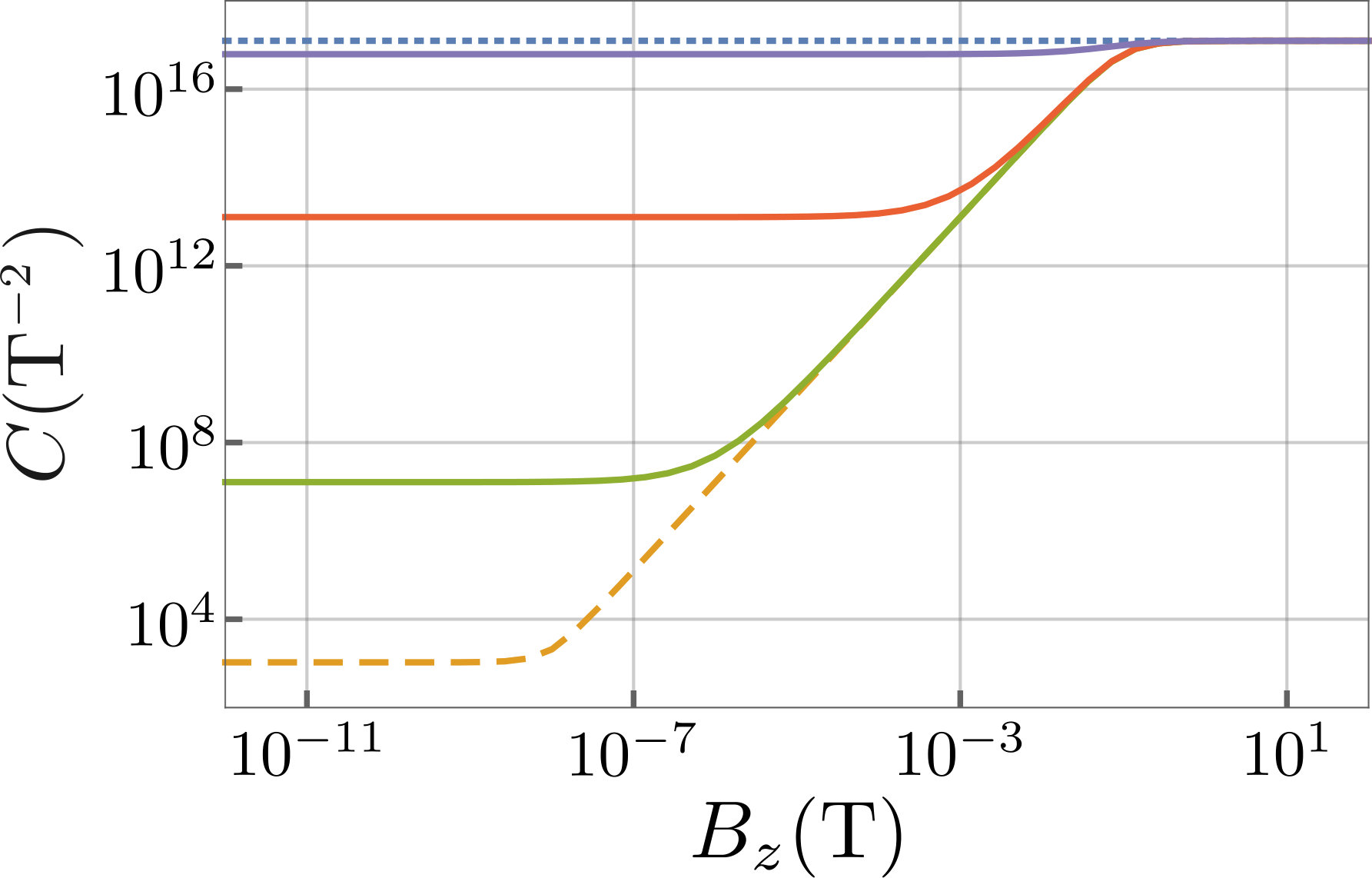 Figure 1
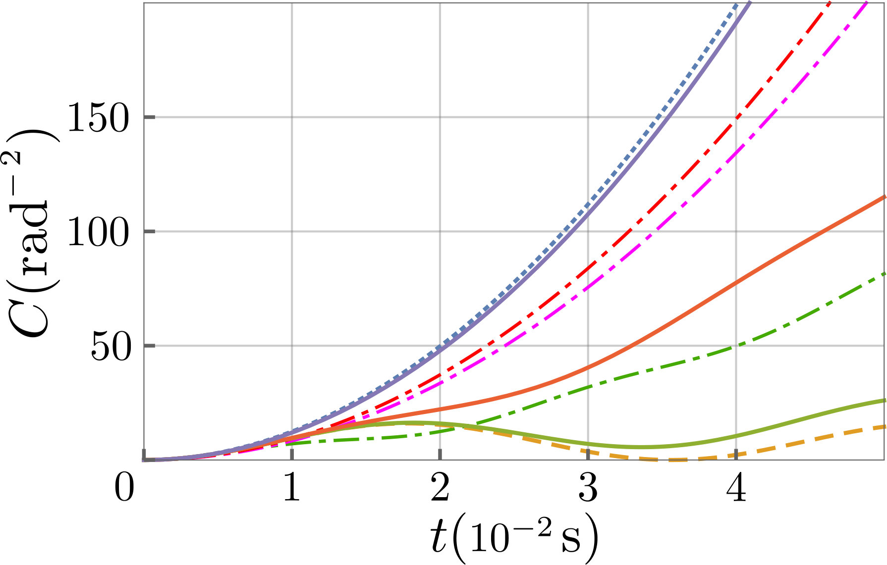 Figure 2
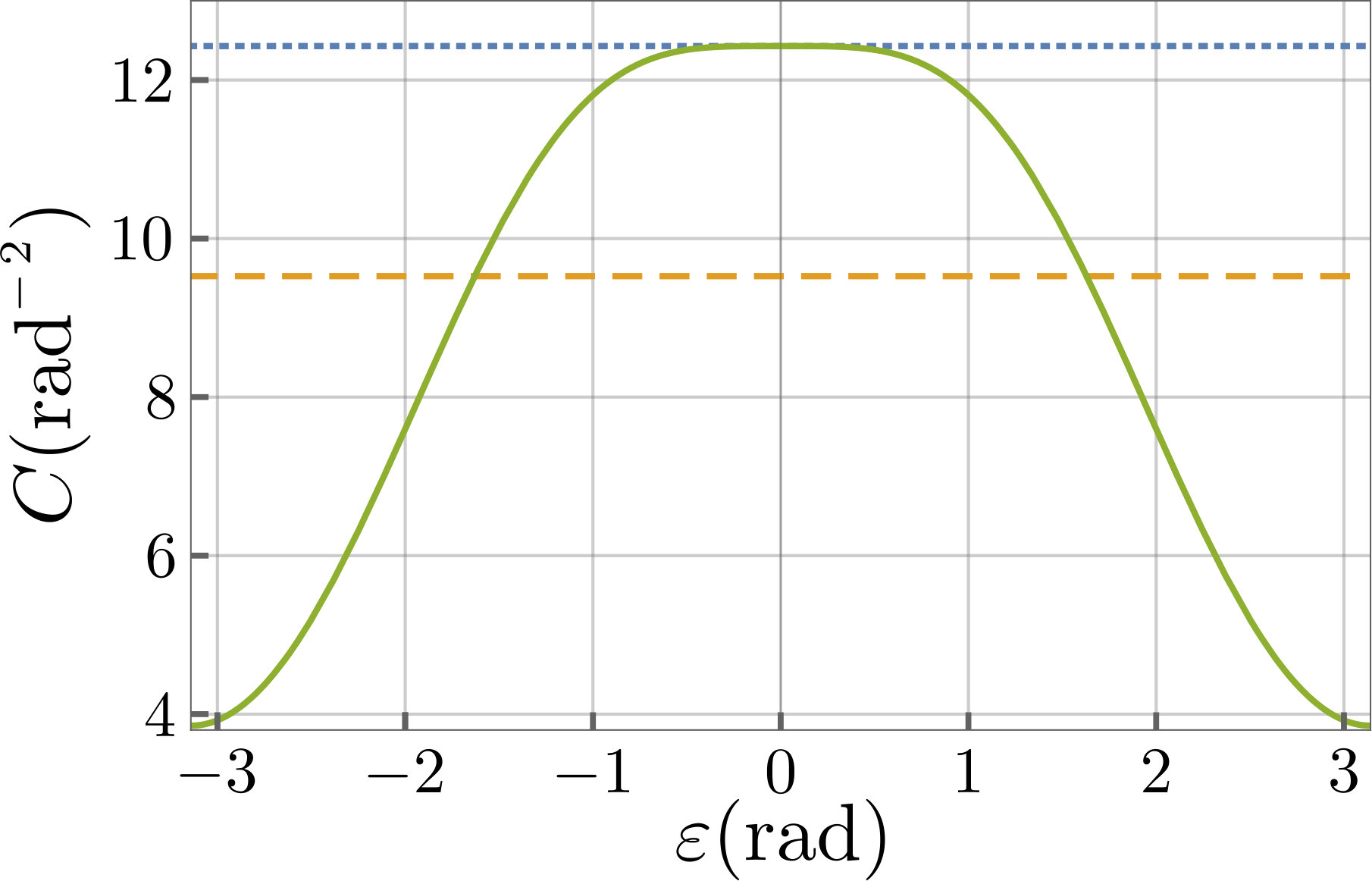 Figure 3
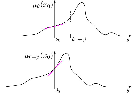 Figure 4
Peer Reviews
No public reviews on file for this paper yet. If you reviewed it on a platform where reviews are public (OpenReview, ICLR, NeurIPS, ICML), you can paste yours below so the community can read it here.
Videos
No videos yet. Explain this paper in a talk, walkthrough, or lecture? Add one.
Enhancing sensitivity in quantum metrology by
Hamiltonian extensions
Julien Mathieu Elias Fraïsse1 and Daniel Braun1
1 Eberhard-Karls-Universität Tübingen, Institut für Theoretische Physik, 72076 Tübingen, Germany
Abstract
A well-studied scenario in quantum parameter estimation theory arises when the parameter to be estimated is imprinted on the initial state by a Hamiltonian of the form . For such “phase shift Hamiltonians” it has been shown that one cannot improve the channel quantum Fisher information by adding ancillas and letting the system interact with them. Here we investigate the general case, where the Hamiltonian is not necessarily a phase shift, and show that in this case in general it is possible to increase the quantum channel information and to reach an upper bound. This can be done by adding a term proportional to the derivative of the Hamiltonian, or by subtracting a term to the original Hamiltonian. Neither method makes use of any ancillas which shows that for quantum channel estimation with arbitrary parameter-dependent Hamiltonian, entanglement with an ancillary system is not necessary to reach the best possible sensitivity. By adding an operator to the Hamiltonian we can also modify the time scaling of the channel quantum Fisher information. We illustrate our techniques with NV-center magnetometry and the estimation of the direction of a magnetic field in a given plane using a single spin-1 as probe.
I Introduction
With the increasing ability of controlling quantum systems, quantum metrology has become a major and lively field. One important task in quantum metrology is the parameter estimation of quantum channels, also known as quantum channel estimation. It is important for at least two reasons. Firstly, because to carry out experiments, it is crucial to know exactly the processes applied to the system. Channel estimation is then used as quantum process tomography. Secondly, quantum channel estimation is useful for investigating the utility of a system for measuring some relevant physical quantity, and for increasing the sensitivity of sensors.
The field has attracted a lot of attention when it became clear that for a given number of probes using entanglement between the probes can increase the sensitivity compared to the classical case Vittorio Giovannetti, et al. (2004); Giovannetti et al. (2006). A second possibility of using entanglement is to introduce an ancillary system and to entangle it with the original system, while still applying the quantum channel only to the original system. It was shown that such channel extensions can sometimes enhance the sensitivity Fujiwara (2001); D’Ariano et al. (2001), in the sense of increasing the Quantum Fisher Information (QFI).
Among quantum channels, unitary channels play a particular role. In these, the time evolution is obtained through propagation with a unitary operator, obtained through the Hamiltonian that depends on the parameter to be estimated, and quantum channel estimation for unitary channels is therefore also known as Hamiltonian parameter estimation. Phase-shift Hamiltonians correspond to the special case where the parameter to be estimated multiplies a Hermitian generator. The corresponding parameter estimation problem is particularly relevant due to the importance of phase measurements in physics. A typical example of such a situation is the estimation of a phase in an interferometer. For unitary channels, we can go beyond channel extension by adding an arbitrary parameter-independent operator to the Hamiltonian, which may include even interactions with ancillary systems that can be initially entangled with the original system. Adding a parameter-independent Hamiltonian to the original Hamiltonian is known as “Hamiltonian extension” Fraïsse and Braun (2016). For phase shifts, Hamiltonian extension does not improve the best possible sensitivity. This was shown in Boixo et al. (2007); Fraïsse and Braun (2016) by calculating an upper bound for the QFI for unitary channels and showing that the bound is saturated for phase shift Hamiltonians.
Here we investigate the problem of saturating the upper bound calculated in Boixo et al. (2007); Fraïsse and Braun (2016) for general Hamiltonians, where it is typically not saturated yet, by extending the Hamiltonian. Indeed, from a pure metrological point of view it is interesting to check whether or not one can go beyond the optimization over initial state and POVM measurement by engineering also the Hamiltonian to increase the sensitivity, without introducing additional parameter dependence. In particular, one would like to know whether ancilla-assisted schemes can provide an advantage for general Hamiltonian parameter estimation. We find that for general parameter dependent Hamiltonians, the sensitivity can be increased by adding a part to the Hamiltonian given by its local derivative with respect to the parameter, multiplied with a large, parameter-independent prefactor. This can be understood intuitively as a “signal flooding”, i.e. the relative weight of the useful part of the Hamiltonian is enhanced. A second way to saturate the upper bound, is to subtract the Hamiltonian taken at a fixed value of the parameter from the original Hamiltonian. At this specific value of the parameter the new Hamiltonian saturates the upper bound. Neither scheme needs any ancillas.
A third opportunity for Hamiltonian extension exists if the eigenvalues of the Hamiltonian are independent of the parameter. This leads to a periodic time-dependence of the channel QFI. An addition to the Hamiltonian that breaks the parameter-independence of the eigenvalues can create a quadratic time scaling in the channel QFI and hence for large enough times strongly increase the sensitivity. While typically this method does not saturate the upper bound, it is still useful for metrology as it allows one to use time as a resource. The engineering of the time scaling to obtain the scaling was also shown in the context of metrology with feedback controls Yuan and Fung (2015); Yuan (2016).
We illustrate our results with NV-center magnetometry, where we find that optimal sensitivity can be reached by adding a strong external magnetic field in the direction of the field to be measured, i.e. flooding the signal with a strong known signal of the same kind. No ancillas are required to reach optimal sensitivity. We also study the qualitatively different estimation of a direction of a magnetic field with a single spin-1 as a probe which allows us to compare the three different methods.
II Quantum metrology
II.1 Channel QFI
In parameter estimation theory, the goal is to infer the value of a parameter given the realization of an -sample of a random variable whose distribution depends on . This is done by an estimator . A common property required for estimators is to be unbiased, meaning that in an infinitesimal interval about the true value of the parameter , on average the estimator should give that true value of the parameter, . A second desirable property is to have a variance as small as possible, such that the estimate fluctuates as little as possible about the true value of the parameter.
Parameter estimation theory applies naturally to the metrology of quantum systems. The most general measurements correspond to POVMs (Positive Operator Valued Measure), i.e. sets of positive semi-definite operators fulfilling the closure relation . Given a state , a POVM generates a probability distribution , mapping the problem of estimating a parameter of a quantum state to the problem of parameter estimation. This approach leads to a fundamental theorem, known as the quantum Cramér-Rao theorem Helstrom (1969); Braunstein and Caves (1994), which sets a bound on the variance of any unbiased estimator given a state ,
[TABLE]
with the Quantum Fisher Information (QFI), defined as . The so-called symmetric logarithmic derivative is defined implicitly by . The bound results from a double optimization: a first optimization over all unbiased estimators, and then a second optimization over all possible POVMs. When repeating the measurement times independently — which amounts to generating an -sample — the quantum Cramér-Rao theorem reads . The bound can always be saturated in the limit of large numbers of measurements by using the maximum likelihood estimator and building the POVM based on the eigenvectors of .
Often the parameter to be estimated characterizes a physical process, i.e. a quantum channel: One starts with an initial state of the probe that is independent of the parameter. Then we let the quantum channel act on the probe, giving as a result the state . A POVM measurement is then performed, whose outcome is fed into and provides us with an estimate of . We see that in this case we have a new degree of freedom in the QFI, the choice of the initial state. One thus introduces a new quantity, the channel QFI , which corresponds to the largest QFI reachable for a given channel,
[TABLE]
Importantly, due to the convexity of the QFI, it is enough to maximize over pure states, .
II.2 Channel extensions and Hamiltonian extensions
We now turn our attention to extensions for metrology. It has been shown that by adding an ancilla to the probe but still acting only with the channel on the probe, i.e. applying to the whole system, one can, for certain channels, improve the channel QFI D’Ariano et al. (2001); Fujiwara (2001). We call such extensions “channel extensions”, in contrast to “Hamiltonian extensions”, defined below. For unitary channels, channel extensions do not increase the channel QFI: (see section III.1 for a short proof).
But when extending the Hamiltonian by adding to it another parameter-independent Hamiltonian ,
[TABLE]
we are not anymore in the situation covered by channel extension. Eq.(3) is our formal definition of a “Hamiltonian extension”. can be a coupling between the original system and an ancilla, but can also refer to a Hamiltonian that acts non-trivially only on the Hilbert space of the original system or on the Hilbert space of the ancilla. Can such a Hamiltonian extension lead to an improvement in the channel QFI? It was shown in Fraïsse and Braun (2016) that for the specific case of phase shift Hamiltonians, i.e. Hamiltonians of the form , such Hamiltonian extensions cannot improve the channel QFI, a result that was already known in the context of many-body interaction metrology Boixo et al. (2007). Here we investigate the question more generally for arbitrary Hamiltonians .
III Metrology with unitary channels
III.1 Channel QFI and semi-norm
From now and for the rest of the article we will focus on unitary channels. These channels correspond to the unitary evolution of the state of a closed system described by the Schrödinger equation. Given the Hamiltonian , the effect of the channel on the initial state is given by with the evolution operator (we take throughout the paper apart from the section V). Since we only deal with unitary channels we adopt the notation for the channel QFI. In general, calculating the QFI is a difficult task as it requires one to diagonalize the density matrix. For pure states the expression is still simple and reads, , where here and throughout the article the dot stands for the derivative with respect to the parameter to be estimated, i.e. . Introducing the local generator
[TABLE]
we can write the QFI as
[TABLE]
with , and consequently the channel QFI as
[TABLE]
The maximization Giovannetti et al. (2006) can be done as follows: Using Popoviciu’s inequality Popoviciu (1935), which states that for a random variable , with minimal value and maximal value , the variance of is upper bounded by , and then noticing that in eq.(5) the variance saturates its upper bound for states of the form (where and correspond, respectively, to eigenvectors of with maximal eigenvalue () and minimal eigenvalue ()), we have
[TABLE]
In order to simplify the calculation of the channel QFI, and following the method in Boixo et al. (2007), we introduce the semi-norm
[TABLE]
with and the maximal and minimal eigenvalues of (we call such eigenvalues extremal eigenvalues, and their associated eigenvectors, extremal eigenvectors ; we also call maximal (resp. minimal) eigenvector an eigenvector corresponding to a maximal (resp. minimal) eigenvalue). We then have the simple expression for the channel QFI
[TABLE]
As it will be important in the following, let us show the triangle inequality for this semi-norm. Let . Then , with (resp. ) a maximal (resp. minimal) eigenvector of . By definition and with and the maximal and minimal eigenvalues of . In the same way we have and with and the maximal and minimal eigenvalues of . We thus get which is exactly the triangle inequality. When and have no degenerate extremal eigenvalues the equality is reached for and , meaning that both operators have to share the same extremal eigenvectors. For the degenerate case, the triangle inequality is saturated if and only if the intersection of the invariant subspaces of the maximal (resp. minimal) eigenvalue of and of is not empty 111Say is an operator acting on . Then a subspace is an invariant subspace of if and only if . We also say that is stable by . Stated otherwise, and should share (in the sense of proportionality) at least one maximal and one minimal eigenvector. Since the eigenvalues are preserved by similarity transformations, we also have for any unitary , regardless of whether depends on or not.
We can use eq.(9) to show that channel extension does not increase the channel QFI of unitary channels: For a unitary channel the extended channel can be written as . We furthermore have showing that , using eq.(9) plus the fact that has the same eigenvalues as .
III.2 Upper bound for the channel QFI
Lemma 1** (Upper bound for channel QFI Boixo et al. (2007)).**
For general Hamiltonians , with associated evolution operator , the channel QFI is upper bounded as
[TABLE]
Lemma 2** (Saturation of the bound).**
In the case where has no degenerate extremal eigenvalues, equality in (10) is reached if and only if the extremal eigenvectors of are also eigenvectors of .
In the degenerate case, equality in (10) is reached if and only if there exist and such that and for all with (resp. ) the invariant subspace of associated with its maximal (resp. minimal) eigenvalue, and where . A sufficient condition is that there exists an eigenvector of in and another one in .
The inequality is saturated by with and , i.e. a balanced superposition of a maximal eigenvector and a minimal eigenvector of .
Proof of Lemma 1Boixo et al. (2007).
In general Wilcox (1967); Snider (1964), for a matrix depending on the parameter , the derivative of its exponential with respect to is given by
[TABLE]
From this expression we can re-express the local generator of the translation,
[TABLE]
with , where . Applying the triangle inequality to the semi-norm of , and noticing that we obtain
[TABLE]
∎
Proof of Lemma 2.
Since is Hermitian, so is and we can then write it in its orthonormal eigenbasis as , with for all , where is the dimension of the invariant subspace of maximal eigenvalue and is the dimension of the invariant subspace with minimal eigenvalue. Since is related to by a similarity transformation, we can write it as with . The condition for equality in eq.(13) and hence in eq.(10) is that there exists a vector which is an eigenvector of with eigenvalue simultaneously for all values of , and a vector which is an eigenvector of with eigenvalue simultaneously for all values of .
Consider first the case where has no degenerate extremal eigenvalues, i.e. and . Then the condition for equality is equivalent to and being eigenvectors of for all . Let us see how we can re-express this condition so that it only involves eigenvectors of and . By expressing the Hamiltonian in its eigenbasis, , we can write . The eigenvectors of are also eigenvectors of but not the other way round: Indeed, may be equal to while . In such cases we can construct eigenvectors of which are not eigenvectors of by linearly combining and . Nevertheless this can happen only for a countable number of -values given , whereas in all other cases the eigenvectors of must also be eigenvectors of . Hence, the condition cannot be satisfied for all if , and therefore the condition for equality in (13) can be stated as: and should be eigenvectors of .
In the degenerate case the eigenspace of with eigenvalue is spanned by . The existence of a common eigenvector of for with eigenvalue means that there should exist a vector independent of that can be written as where the last equality defines . Since this is equivalent to say that there should exist a vector such that belongs to for . This is true especially for showing that also belongs to . A similar treatment for the lowest eigenvalue shows that the necessary and sufficient condition for equality in eq.(10) is equivalent to the existence of a vector such that for , and of a vector such that for . The sufficient condition is found by observing that the above condition is fulfilled if has an eigenvector in and an eigenvector in . ∎
In the case of phase shifts, the condition for equality in eq.(10) is fulfilled as and are simultaneously diagonalizable, showing that for phase shifts . The Hamiltonian extension of a phase shift is not a phase shift anymore. We thus have , showing that quantum metrology with phase shift Hamiltonians cannot profit from Hamiltonian extension, in addition to not being able to profit from channel extensions.
IV Saturating the bound
We have seen that Hamiltonian extension fails to provide an advantage in terms of channel QFI for phase shift Hamiltonians. Nevertheless the question of the order between and is still open for arbitrary Hamiltonians , where is the local generator of the extended Hamiltonian with . We only have the two inequalities
[TABLE]
where the second one follows from the fact that is independent of . The interesting question here is thus whether for a given that does not saturate (14) we can saturate the bound (15) by tuning the interaction Hamiltonian in , and therefore increase the sensitivity, i.e. have . To answer this question, we first look at the specific case of what we call “broken phase-shift” before treating the general case.
IV.1 Restoring a broken phase shift
Let us consider the Hamiltonian , along with the corresponding unitary operator and the corresponding local generator . For we have from eq.(10) . We assume that the conditions for equality in eq.(10) are not fulfilled and we therefore have . Our goal is to design a Hamiltonian extension for such that the channel QFI for saturates inequality (10), i.e.
[TABLE]
In order to saturate the bound two solutions appear directly. Loosely speaking, we can either cancel the part that spoils the Hamiltonian, , or increase the useful part of the Hamiltonian, . Both of them correspond to a Hamiltonian extension but without ancillas, just adding an extra part to the Hamiltonian. In the first case the extra Hamiltonian is , and the corresponding extended Hamiltonian becomes the phase shift , which saturates the bound (16). While this method may appear artificial, it clearly demonstrates the possibility of enhancing the sensitivity in the case where the parameter is not coded in a simple phase shift. In fact, it is not even necessary to add the full . Assuming for simplicity non-degenerate extremal eigenvalues of , we know from Lemma 2 that only the extremal eigenvectors of have to be eigenvectors of . With this one shows easily that a corrected saturates the upper bound if and only if for with and for with . I.e. loosely speaking, needs to be substracted only in the subspace of the extremal eigenvectors.
The second strategy is to add a Hamiltonian . The extended Hamiltonian in this case reads , i.e. we have . Hence, for large , the eigenvectors of become those of , i.e. and have then the same extremal eigenvectors and the bound (16) can be saturated. Importantly, this transformation does not correspond to just a re-parametrization: In a re-parametrization we keep the same probability distribution, and we only change what we consider to be the parameter of the probability distribution. In the present case we change the probability distribution, but we keep the original parameter, since it corresponds to the physical quantity in which we are interested.
Let us formalize this in terms of Fisher Information (FI). We consider the distribution . The FI of this distribution for the parameter at the point is . If we now consider a new parameter , then the FI for the same probability distribution at is given by
[TABLE]
In the case of a shift of the parameter, say we get and the FI is not changed. This corresponds to the intuitive picture that by just changing what we consider to be the parameter in the probability distribution we do not really gain more information.
Fundamentally different is the change of the probability distribution. Consider the new probability distribution . Then the FI of the new distribution, still for the same parameter , is given by
[TABLE]
In the specific case of a shift of the parameter in the probability distribution, we obtain
[TABLE]
This means that when we use the new distribution , the resulting FI at equals the FI of the original distribution at the point (see Figure 1).
If we now go back to physics, and if we consider to be a free parameter, then we can tune it to work at the most favorable position of the Hamiltonian in terms of . In the case of the broken phase shift, the most favorable values of are the large values of , where the effect of the term becomes negligible. Then, whatever is the original value of we can, by adding the Hamiltonian and taking arbitrarily large, approach arbitrarily the upper bound of the QFI.
IV.2 Maximum sensitivity by "Signal flooding"
We have seen that in order to saturate the upper bound of the channel QFI for the "broken phase shift", , we can add a Hamiltonian proportional to , the generator of the original phase shift. This generator corresponds to the first derivative of the total Hamiltonian . We show in this section that this is actually a general result: By adding a term proportional to the first derivative of the Hamiltonian, we can bring the channel QFI arbitrarily close to its upper bound. We denote the extended Hamiltonian obtained in this way as
[TABLE]
Instead of working directly with the channel QFI we first consider the QFI for an arbitrary pure state. Starting with an initial state the QFI is given by
[TABLE]
with the local generator and the evolution operator . The important part in this expression is the derivative of the evolution operator. Using eq.(11) we can write it as
[TABLE]
The derivative of the evolution operator with respect to is independent of the value of and equals
[TABLE]
and since , we have
[TABLE]
We thus have
[TABLE]
i.e. the QFI for at is equal to the QFI for at . In the limit of large we have . This Hamiltonian is, with respect to , a phase shift Hamiltonian which implies that . Since eq.(24) is true for all states , it is also true for the channel QFI, i.e. , showing in fine that “signal flooding” allows one to saturate the upper bound for the channel QFI,
[TABLE]
The interpretation of this result follows from Lemma 2: by adding a large term proportional to to , we bring the eigenvectors of close to those of . When the added part dominates completely the Hamiltonian the conditions for equality given in the Lemma 2 are fulfilled, and the bound is saturated. Of course, for applying this method, in general we need to know the value of already in order to be able to add the Hamiltonian . But the situation is not worse than what one encounters when optimizing the POVM, which through usually also depends on : The framework of the QFI and its operational meaning are local, but the QFI is still a useful quantity. One typically assumes that we know already "roughly" the value of and that knowledge can be used to find a near-optimal POVM. In the present context, we would also use this prior knowledge to determine the Hamiltonian to be added. Moreover, for the physically important case of a broken phase shift, is independent of , and hence no knowledge at all of is required for flooding the signal. We emphasize that the Hamiltonian we add does not depend on , but only on . Adding a Hamiltonian that depends on may for sure increase the channel QFI to values actually larger than the upper bound, but requires not only prior information, but also the need to design a way to add an extra dependence on the parameter. This would be comparable to adding an extra dependence on the parameter through a -dependent POVM Seveso et al. (2017).
IV.3 Subtracting the Hamiltonian
The first method discussed in section IV.1 in the context of a broken phase shift, namely subtracting the disturbing part from the Hamiltonian can be generalized further: We can subtract the entire Hamiltonian at from the Hamiltonian, leading to a new Hamiltonian
[TABLE]
This is a valid Hamiltonian extension in the sense that we added a -independent operator to the Hamiltonian while keeping its parametric derivative, . Moreover, at this Hamiltonian vanishes, , and therefore commutes with any operator, in particular with its own derivative, . This implies that we thus saturate the bound:
[TABLE]
In full generality we can subtract , with and still saturate the bound. Below we show for the example of the measurement of the direction of the magnetic field how a locally vanishing Hamiltonian can be realized.
We now check how stable the method is if one does not subtract exactly but rather . We define the extended Hamiltonian . To second order in we have
[TABLE]
To obtain the channel QFI we need the eigenvalues of , the local generator corresponding to . Using in eq.(11) and the fact that , we obtain, up to second order,
[TABLE]
where . We can now use perturbation theory to see how the eigenvalues of are affected by . In its eigenbasis, is written . We denote the eigenvalues of by . Assuming non-degenerate , we have to first order perturbation theory in
[TABLE]
Provided that is small enough, no new degeneracies will appear. If and are respectively the maximal and minimal eigenvalue of , then the channel QFI of the extended channel is given up to second order in by
[TABLE]
This shows that errors of the order in the value of lead to a channel QFI reaching the upper bound up to a correction of order .
It was shown in Yuan and Fung (2015) that one can also saturate the upper bound with a different method: by breaking the evolution operator in evolution operators with evolution time , and interspersing controls one can increase the channel QFI. An optimal choice of controls leads to the saturation of the upper bound. Neither of the three methods signal flooding, using additional interspersed controls, and Hamiltonian subtraction makes any use of ancillas. This shows that in all generality, ancillas are not necessary to achieve the maximal sensitivity when estimating a Hamiltonian parameter. While this result was already known for phase shift Hamiltonians Boixo et al. (2007); Fraïsse and Braun (2016), these methods show that it is the case for any Hamiltonian.
IV.4 Engineering the time dependence of the channel QFI
Hamiltonian extension can also be used to modify the behavior of the channel QFI with time or other relevant resources. It was shown in Pang and Brun (2014, 2016) that in case the eigenvalues of the Hamiltonian do not depend on the parameter to be estimated, the QFI behaves periodically in (this discussion on applies actually to any phase shift parameter). In general for (we assume for simplicity the Hamiltonian non-degenerate) the local generator is given Pang and Brun (2014) by
[TABLE]
clearly showing that if , i.e if the eigenvalues of are -independent, only the periodic term survives. The fact that the channel QFI (and more generally the QFI) behaves only periodically with the time prohibits the use of time as a resource: We cannot increase the sensitivity to arbitrarily large values by increasing the evolution time. This is particularly harmful since quantum metrology typically provides a quadratic scaling with time (for time-independent Hamiltonians), to be compared to the linear scaling obtained by classical averaging.
To show how Hamiltonian extension can help to engineer the time dependence we assume that the eigenvalues of the original Hamiltonian do not depend on : . We then consider the Hamiltonian extension
[TABLE]
where can be any operator. For small we can use the perturbation theory to first order to find the perturbed eigenvalues of . Assuming non-degenerate , we have
[TABLE]
We see that the introduction of in the Hamiltonian makes the eigenvalue depend on , as long as is not constant as function of . Under this condition this Hamiltonian extension introduces a quadratic scaling with time in the QFI. Despite the fact that for a general this Hamiltonian extension does typically not allow one to saturate the upper bound it offers the advantage that one does not need to know the exact value of the parameter to implement it.
The method of engineering the time dependence shows that in general, not only can be used to increase the channel QFI. One can check case by case if adding another operator helps to increase the best sensitivity. For example it was shown for a broken phase shift of the form that the channel QFI is not always a monotone function of De Pasquale et al. (2013). Thus, for certain values of the channel QFI can be increased by increasing , an effect that the authors call “dithering”.
V Example of applications
V.1 NV center magnetometry
The nitrogen-vacancy defects in diamonds, also known as NV centers, correspond to defects in a diamond crystal lattice, where a substitutional nitrogen atom comes with a vacancy in one of the neighbouring sites. Such NV centers exist in three forms, a neutral one, a positively charged one, and a negatively charged one. The latter provides a promising system for magnetometry, since it has a spin triplet which can be monitored efficiently through optical processes, and offers a coherence time that can be as high as a few ms (see Schirhagl et al. (2014); Rondin et al. (2014) for recent reviews).
Neglecting the interactions with the 14N nuclear spin as well as the bath of the 13C nuclear spins, the Hamiltonian for the triplet state of the NV center can be written Rondin et al. (2014)
[TABLE]
with the Landé factor, the Bohr magneton, and the zero field splitting parameters and and the dimensionless spin-1 matrices, fulfilling . The zero field splitting has two components, the axial one, with parameter (taken as GHz), and the off-axis one, with parameter (taken as MHz). The parameter that one seeks to estimate is , the magnetic field in the direction which is the direction of the axis from N to V. This Hamiltonian has the form of a "broken phase shift" with . The channel QFI is bounded by . Due to the part which does not commute with , i.e. the magnetic transverse field and the off-axis zero field splitting, the channel QFI decreases for small value of , while for high values of the channel QFI reaches the upper bound (see Figure 2).
As we have seen in section IV, by adding the derivative of the Hamiltonian to the original Hamiltonian we can saturate the upper bound. The shifted Hamiltonian is
[TABLE]
We represent in Figure 2 the effect of on the channel QFI. We see that by increasing the value of we can get arbitrarily close to the upper bound. As pointed out when discussing the "broken phase shift", the effect of amounts here to evaluating the QFI at shifted value of the parameter (at instead of at ). For magnetometry with NV-centers it is actually already known that adding an additional magnetic field can help to measure weak magnetic fields. In Rondin et al. (2014) this was discussed in the the context of reaching a linear Zeeman effect. In addition, adding a bias field makes already sense from the perspective of shifting the precession signal up to higher frequency, where it can be distinguished from noise more easily. Here we see that independently of such specific considerations, “flooding the signal” by adding the known parameter-derivative of the Hamiltonian with a large factor is a very general method that allows one to overcome pernicious effects of other parts of the Hamiltonian and reach maximal possible sensitivity.
The behaviour of the channel QFI for very low values of deserves some more comments. As it can be seen in Figure 2 when becomes very small the channel QFI reaches a plateau. This is a quite general feature for Hamiltonians of the form of a "broken phase shift" . The channel QFI at can be obtained by calculating which reads
[TABLE]
with , where the s and the s are respectively the eigenvalues (assumed non-degenerate here) and eigenvectors of , and , with . To get more insight into this expression notice that the channel QFI vanishes only when maximal and minimal eigenvalues of coincide, i.e. when is proportional to the identity operator. In general this will be the case if is an integer and . This condition is not necessary since can be sparse and therefore some may already be equal to zero. Still, this simple analysis shows that particular cases excepted, it is a quite general feature that the channel QFI for a broken phase shift does not vanish for small values of the parameter.
V.2 Estimation of a direction of a magnetic field
The estimation of a component of a magnetic field using a NV center studied in the previous section leads to a broken phase shift. We now consider the estimation of one of the spherical angles characterizing the direction of a magnetic field with a free spin-1 as a probe, a situation that does not correspond to a broken phase shift. The Hamiltonian is given by
[TABLE]
with and . We want to estimate the parameter in a scalar parameter setting (we consider and as known). The channel QFI for the corresponding channel is bounded as
[TABLE]
The eigenvalues of are [math] and , from which we get . The local generator of the translation in can be computed exactly and its eigenvalues are [math] and . This gives a channel QFI equal to
[TABLE]
We see that the channel QFI has a periodic time dependence since the eigenvalues of are -independent (see dashed line in Figure 3). However, the upper bound still scales quadratically with time. As a result, for large time, the discrepancy between the actual channel QFI and its upper bound increases. Notice that for this Hamiltonian the role of time in the channel QFI is the same as the role of the strength of the magnetic field.
V.2.1 Signal flooding
We now examine how "signal flooding" helps to increase the channel QFI. We consider the extended Hamiltonian
[TABLE]
We represent in the Figure 3 the effect of signal flooding by plotting the channel QFI of for different values of . In the same way as for the NV center Hamiltonian we see that increasing the value of allows one to get arbitrarily close to the upper bound. In contrast to the estimation of a broken phase shift (e.g. estimation of for the NV center), here signal flooding does not correspond to a shift of the value of .
V.2.2 Time engineering
Having eigenvalues independent of , leads to a channel QFI with a periodic time scaling. In line with section IV.4 we now show how we can restore the quadratic time scaling using a Hamiltonian extension. We consider the extended Hamiltonian
[TABLE]
which correspond to the original Hamiltonian with an additional magnetic field in the direction with a strength .
The eigenvalues of are [math] and , showing that the additional magnetic field makes the eigenvalues depend on , and therefore allow one to create a quadratic time scaling. We have represented in Figure 3 the channel QFI of the extended Hamiltonian for different values of . This clearly shows that the additional magnetic field introduces a quadratic scaling, but also that the larger , i.e. the strength of the additional field, the larger is the channel QFI. In contrast to signal flooding, for very large values of we do not reach the upper bound (compare the case and ): Indeed do not fulfil the condition of Lemma 2 and when it dominates completely the Hamiltonian we do still not reach the upper bound.
V.2.3 Hamiltonian subtraction
Finally, we show how we saturate the upper bound using Hamiltonian subtraction. Hamiltonian subtraction here amounts to adding a magnetic field of the same strength but in opposite direction to the original magnetic field. To see the effect of a slight deviation from the correct direction of the added field, we study the perturbed Hamiltonian
[TABLE]
We can calculate the channel QFI exactly,
[TABLE]
One verifies that for values of this saturates the upper bound (39). It is interesting to notice that the correction of second order in in the channel QFI vanishes exactly, and the leading order corrections are of order , demonstrating the stability of the method to perturbation in the direction of the subtracted magnetic field, as represented in Figure 4.
VI Conclusion
We investigated the problem of single Hamiltonian parameter estimation, and the effect of Hamiltonian extension on the precision with which one can estimate the parameter. It was already known that in the case of a phase shift, Hamiltonian extension does not lead to an increase of the channel QFI (QFI optimized over all input states) Fraïsse and Braun (2016); Boixo et al. (2007). But for more general Hamiltonians, Hamiltonian extension may increase the channel QFI. In particular, we found two ways of engineering the Hamiltonian to saturate the upper bound of the channel QFI: ()"Signal flooding" which consists of adding to the original Hamiltonian a large term proportional to its derivative; and "Hamiltonian subtraction" which consists in subtracting the Hamiltonian at a fixed value of the parameter from the original Hamiltonian.
Neither method makes use of any ancillas, showing that adding subsystems is in general not necessary for unitary parameter estimation to achieve the best precision. We applied "signal flooding" to the Hamiltonian of an NV center. Such systems are used to measure small magnetic fields. We showed how adding a magnetic field in the -direction helps to increase the maximal possible sensitivity of the measurement of the magnetic field’s component in the same direction. We also illustrated both methods with the estimation of a direction of a magnetic field.
Finally we showed that in cases where the eigenvalues of the original Hamiltonian are parameter-independent, adding almost any constant Hamiltonian can lead to a quadratic increase of the channel QFI with time, whereas for the original Hamiltonian it is bounded and periodic in time. Such is the situation for the measurement of the polar angle of the magnetic field, probed with a free spin. This will typically not enable saturation of the bound of the channel QFI, but can nevertheless be very advantageous for large measurement times, and relatively straight-forward to implement.
The scenario considered in this work is an ideal one. Our figure of merit, the channel QFI, constitutes a valid and achievable benchmark for quantum parameter estimation that is difficult to reach in practice. Even if the theory gives us the optimal POVM and the optimal state, they may be hard to implement. Therefore, it may be interesting to see to what extend Hamiltonian extensions also work in situations where the optimal POVM or the optimal state cannot be implemented. Acknowledgment We thank Fabienne Schneiter for useful discussions.
The reference list from the paper itself. Each links out to its DOI / PubMed record.
- 1Vittorio Giovannetti, et al. (2004) Vittorio Giovannetti,, Seth Lloyd, and Lorenzo Maccone, Science 306 , 1330 (2004).
- 2Giovannetti et al. (2006) V. Giovannetti, S. Lloyd, and L. Maccone, Phys. Rev. Lett. 96 , 010401 (2006) . · doi ↗
- 3Fujiwara (2001) A. Fujiwara, Phys. Rev. A 63 , 042304 (2001) . · doi ↗
- 4D’Ariano et al. (2001) G. M. D’Ariano, P. Lo Presti, and M. G. A. Paris, Phys. Rev. Lett. 87 , 270404 (2001) . · doi ↗
- 5Fraïsse and Braun (2016) J. M. E. Fraïsse and D. Braun, ar Xiv (2016), ar Xiv:1610.05974 [quant-ph] .
- 6Boixo et al. (2007) S. Boixo, S. T. Flammia, C. M. Caves, and J. Geremia, Phys. Rev. Lett. 98 , 090401 (2007) . · doi ↗
- 7Yuan and Fung (2015) H. Yuan and C.-H. F. Fung, Phys. Rev. Lett. 115 , 110401 (2015) . · doi ↗
- 8Yuan (2016) H. Yuan, Phys. Rev. Lett. 117 , 160801 (2016) . · doi ↗