Gravitational collapse to a Kerr-Newman black hole
Antonios Nathanail, Elias R. Most, Luciano Rezzolla

TL;DR
This paper systematically studies the collapse of rotating, magnetised neutron stars into Kerr-Newman black holes, revealing how initial rotation and magnetic fields influence the black hole's charge and properties.
Contribution
It presents the first detailed analysis of how rotating, magnetised neutron stars collapse into charged, rotating black holes under realistic astrophysical assumptions.
Findings
Rotating neutron stars acquire a net charge during collapse.
The resulting black hole is a Kerr-Newman black hole with trapped charge.
Without rotation or magnetic field, collapse results in Schwarzschild or Kerr black holes.
Abstract
We present the first systematic study of the gravitational collapse of rotating and magnetised neutron stars to charged and rotating (Kerr-Newman) black holes. In particular, we consider the collapse of magnetised and rotating neutron stars assuming that no pair-creation takes place and that the charge density in the magnetosphere is so low that the stellar exterior can be described as an electrovacuum. Under these assumptions, which are rather reasonable for a pulsar that has crossed the 'death line', we show that when the star is rotating, it acquires a net initial electrical charge, which is then trapped inside the apparent horizon of the newly formed back hole. We analyse a number of different quantities to validate that the black hole produced is indeed a Kerr-Newman one and show that, in the absence of rotation or magnetic field, the end result of the collapse is a Schwarzschild…
Click any figure to enlarge with its caption.
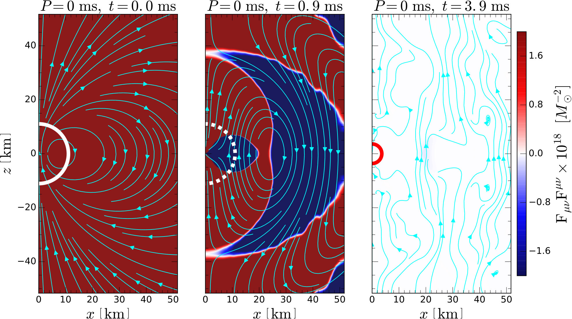 Figure 1
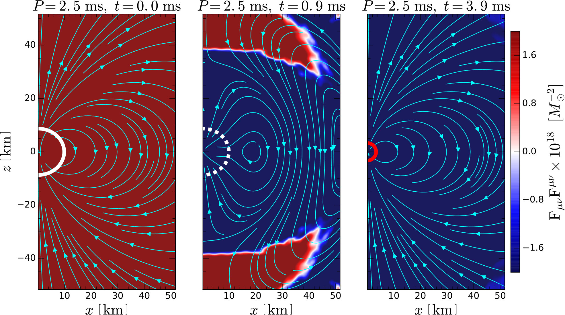 Figure 2
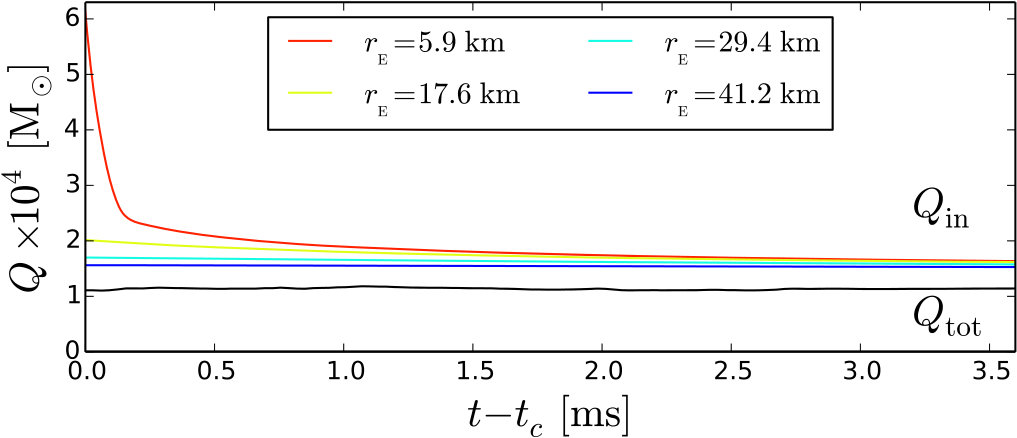 Figure 3
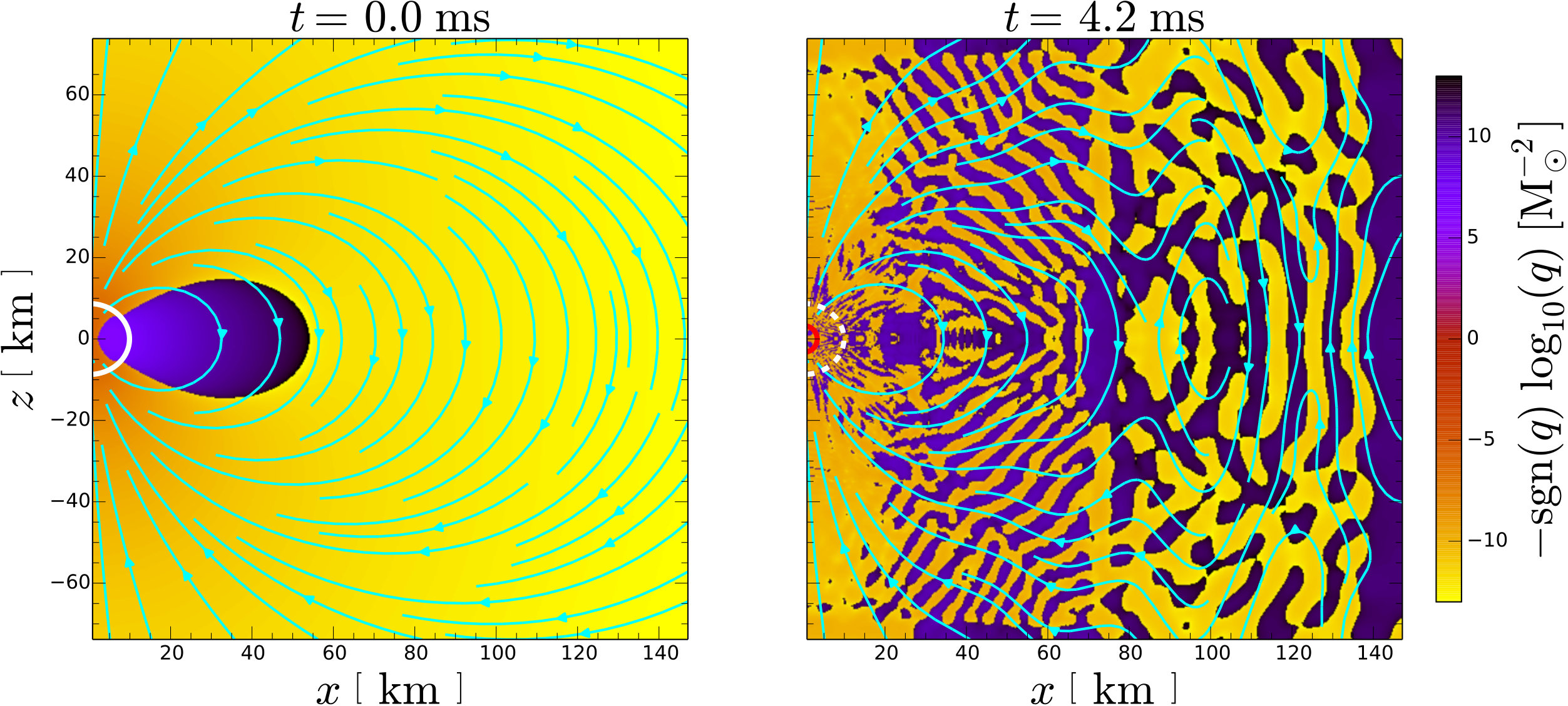 Figure 4
Peer Reviews
No public reviews on file for this paper yet. If you reviewed it on a platform where reviews are public (OpenReview, ICLR, NeurIPS, ICML), you can paste yours below so the community can read it here.
Videos
No videos yet. Explain this paper in a talk, walkthrough, or lecture? Add one.
Gravitational collapse to a
Kerr-Newman black hole
Antonios Nathanail1 , Elias R. Most1, Luciano Rezzolla1,2
1Institut für Theoretische Physik, Goethe Universität Frankfurt, Max-von-Laue-Str.1, 60438 Frankfurt am Main, Germany
2Frankfurt Institute for Advanced Studies, Ruth-Moufang-Str. 1, 60438 Frankfurt am Main, Germany E-mail: [email protected]
Abstract
We present the first systematic study of the gravitational collapse of rotating and magnetised neutron stars to charged and rotating (Kerr-Newman) black holes. In particular, we consider the collapse of magnetised and rotating neutron stars assuming that no pair-creation takes place and that the charge density in the magnetosphere is so low that the stellar exterior can be described as an electrovacuum. Under these assumptions, which are rather reasonable for a pulsar that has crossed the “death line”, we show that when the star is rotating, it acquires a net initial electrical charge, which is then trapped inside the apparent horizon of the newly formed back hole. We analyse a number of different quantities to validate that the black hole produced is indeed a Kerr-Newman one and show that, in the absence of rotation or magnetic field, the end result of the collapse is a Schwarzschild or Kerr black hole, respectively.
keywords:
neutron stars; numerical relativity; black holes; collapsing stars; Kerr-Newman;
††pubyear: 2016††pagerange: Gravitational collapse to a Kerr-Newman black hole–References
1 Introduction
The rotating black-hole (Kerr) solution of the Einstein equations in vacuum and axisymmetric spacetimes is a fundamental block in relativistic astrophysics and has been studied in an enormously vast literature for its mathematical and astrophysical properties. On the other hand, the rotating and electrically charged black hole (Kerr-Newman, KN hereafter) solution of the Einstein-Maxwell equations in axisymmetric spacetimes, while equally well studied for its mathematical properties, is also normally disregarded as astrophysically relevant. The rationale being that if such an object was indeed created in an astrophysical scenario, then the abundant free charges that accompany astrophysical plasmas would neutralise it very rapidly, yielding therefore a standard Kerr solution.
Yet, KN black holes continue to be considered within astrophysical scenarios to explain, for instance, potential electromagnetic counterparts to merging stellar-mass binary black-hole systems (Zhang, 2016; Liebling & Palenzuela, 2016; Liu et al., 2016). We here take a different view and do not explore the phenomenology of KN black holes when these are taken to be long-lived astrophysical solutions. Rather, we are interested to determine how such black holes are produced in the first place as, for instance, in the collapse of rotating and magnetised stars. We note that even if these solutions are short-lived astrophysically (Contopoulos et al., 2014; Punsly & Bini, 2016), the study of their genesis can provide useful information and shed light on some of the most puzzling astronomical phenomena of the last decade: fast radio bursts [FRBs; Lorimer et al. (2007); Thornton et al. (2013)]. FRBs are bright, highly dispersed millisecond radio single pulses that do not normally repeat and are not associated with a known pulsar or gamma-ray burst. Their high dispersion suggests they are produced by sources at cosmological distances and thus with an extremely high radio luminosity, far larger than the power of single pulses from a pulsar. The event rate is also estimated to be very high and of a few percent that of supernovae explosions, making them very common. Several theoretical models have been proposed over the last few years, but the “blitzar” model (Falcke & Rezzolla, 2014), is particularly relevant for our exploration of the formation of KN black holes.
We recall that if a neutron star exceeds a certain limit in mass and angular momentum, it will reach a state in which it cannot support itself against gravitational collapse to a black hole. It is also widely accepted that rotating magnetised neutron stars emitting pulsed radio emission, i.e., pulsars, spin down because of electromagnetic energy losses and could therefore reach the stability line against collapse to a black hole. During the collapse of such a pulsar, an apparent horizon is formed which will cover all the stellar matter, while the magnetic-field lines will snap violently launching an intense electromagnetic wave moving at the speed of light. Free electrons will be accelerated by the travelling magnetic shock, thus dissipating a significant fraction of the magnetosphere energy into coherent electromagnetic emission and hence produce a massive radio burst that could be observable out to cosmological distances (Falcke & Rezzolla, 2014).
One aspect of this scenario that has not yet been fully clarified is the following: does the gravitational collapse of a rotating magnetised neutron star lead to a KN black hole? The purpose of this paper is to provide an answer to this question and to determine, through numerical-relativity simulations, the conditions under which a collapsing pulsar will lead to the formation of a Kerr or a Kerr-Newman black hole. In particular, we show that when using self-consistent initial data representing an unstable rotating and magnetised neutron star in general relativity, the consequent collapse yields a black hole that has all the features expected from a KN black hole. In particular, the spacetime undergoes a transition from being magnetically dominated before the collapse, to being electrically dominated after black-hole formation, which is indeed a key feature of a KN black hole. We further provide evidence by carefully analysing the Weyl scalar and by showing that the black-hole spacetime possesses a net electric charge and a behaviour which is the one expected for a KN black hole. These results will be contrasted with those coming from the gravitational collapse of a nonrotating magnetised neutron star, where the outcome is an uncharged nonrotating (Schwarzschild) black hole.
The plan of the paper is the following one. In Sec. 2 we briefly review the numerical setup and how the initial data is computed, leaving the analysis of the numerical results in Sec. 3. Finally, the discussion of the astrophysical impact of the results and our conclusions are presented in Sec. 4
2 Numerical setup and Initial data
All simulations presented here have been performed employing the general-relativistic resistive magnetohydrodynamics (MHD) code WhiskyRMHD (Dionysopoulou et al., 2013; Dionysopoulou et al., 2015), which uses high-resolution shock capturing methods like the Harten-Lax-van Leer-Einfeldt (HLLE) approximate Riemann solver coupled with effectively second order piece-wise parabolic (PPM) reconstruction. Differently from the implementation reported in Refs. (Dionysopoulou et al., 2013; Dionysopoulou et al., 2015), we reconstruct our primitive variables at the cell interfaces using the enhanced piecewise parabolic reconstruction (ePPM) (Colella & Sekora, 2008; Reisswig et al., 2013), which does not reduce to first order at local maxima. Also, we opt for reconstructing the quantity , where is the Lorentz factor, instead of the 3-velocity ; this choice enforces subluminal velocities at the cell interface. Regarding the electric-field evolution, we choose not to evolve the electrical charge directly through an evolution equation, and instead compute at every timestep, as it has been done by Dionysopoulou et al. (2013) and Bucciantini & Del Zanna (2013). The WhiskyRMHD code exploits the Einstein Toolkit, with the evolution of the spacetime obtained using the McLachlan code (Löffler et al., 2012), while the adaptive mesh refinement is provided by Carpet (Schnetter et al., 2004).
The use of a resistive-MHD framework has the important advantage that it allows us to model the exterior of the neutron star as an electrovacuum, where the electrical conductivity is set to be negligibly small, so that electromagnetic fields essentially evolve according to the Maxwell equations in vacuum. These are the physical conditions that are expected for a pulsar that has passed its “death line”, that is, one for which either the slow rotation or a comparatively weak magnetic field are such that it is not possible to trigger pair creation and its magnetosphere can be well approximated as an electrovacuum (Chen & Ruderman, 1993)111We recall that the voltage drop along magnetic field lines needed for the creation of pairs scales with the magnetic field and rotation frequency simply as (Ruderman & Sutherland, 1975).. At the same time, the resistive framework also enables us to model the interior of the star as highly conducting fluid, so that our equations recover the ideal-MHD limit (i.e., infinite conductivity) in such regions. WhiskyRMHD achieves this by including a current that is valid both in the electrovacuum and in the ideal-MHD limit, where it becomes stiff, however. To accurately treat such a current, the code uses an implicit-explicit Runge-Kutta time stepping (RKIMEX) (Pareschi & Russo, 2005). For more details on the numerical setup we refer the interested reader to Dionysopoulou et al. (2013) and Dionysopoulou et al. (2015).
Our initial data is produced using the Magstar code of the LORENE library, which can compute self-consistent solutions of the Einstein-Maxwell equations relative to uniformly rotating stars with either purely poloidal (Bocquet et al., 1995) or toroidal magnetic fields (Frieben & Rezzolla, 2012); hereafter we will consider only poloidal magnetic fields of dipolar type. We have considered a number of different possible configurations for the electric field with the aim of minimising the amount of external electric charges. In practice, the smallest external charge has been achieved when prescribing a corotating interior electric field matched to a divergence-free electric field produced by a rotating magnetised sphere. More precisely, we set the electric field in the stellar interior using the ideal-MHD condition, i.e., where is the corotation velocity, the 3-metric determinant and the totally antisymmetric permutation symbol. This field is then matched to an exterior electrovacuum solution for a magnetised and rotating uncharged sphere in general-relativity (Rezzolla et al., 2001, 2003). Note that because the analytic solution is obtained in the slow-rotation approximation, which assumes a spherical star, a small mismatch in the electric field is present near the pole. Furthermore, monopolar and a quadrupolar terms are added to the solution so as to match the charge produced by the corotating interior electric field following Ruffini & Treves (1973).
Also, as customary in this type of simulations, the stellar exterior is filled with a very low-density fluid, or “atmosphere”, whose velocity is set to be zero (Dionysopoulou et al., 2013); at the same time, and from an electrodynamical point of view, we treat such a region as an electrovacuum, so that the electrical conductivity is set to zero. This has the important consequence that the magnetic fields are no longer frozen in the atmosphere and are therefore free to rotate following the stellar rotation if one is present.
Our reference rotating model is represented by a neutron star with gravitational mass of , a period of (or ), and a central (and maximum) magnetic field of ; for such a model, the light cylinder is at about from the origin. The corresponding reference nonrotating model has instead a gravitational mass of and the same magnetic field of . Finally, we will also consider a model with the same properties as the rotating one, but with zero magnetic field. All models are constructed from a single polytrope with . The polytropic constant has been adjusted so that the maximum mass of a nonrotating star is limited to about . The evolution is however performed using an ideal-fluid equation of state , where is the specific internal energy. In spite of using a very simplified equation of state, we do not expect this to have any effect on the results of this paper since we are merely interested in a prompt collapse to a black hole.
An important issue to discuss at this point is whether or not the star possesses initially a net electrical charge. As it happens, the standard solution provided by Magstar does have a net charge, although we decided not to use such a solution as it is not the one leading to the smallest external charge. At the same time, it is reasonable to expect that the strong electromagnetic fields in a pulsar will not only generate a charge separation, but they will also lead naturally to a net charge. Assuming, that the rotating neutron star is endowed with a dipolar magnetic field aligned with the rotation axis and that it is surrounded by a ionised medium, it will induce a radial electric field (Cohen et al., 1975; Michel & Li, 1999).
[TABLE]
where is the equatorial value of the dipole magnetic field as measured by a nonrotating observer, while and are the angular velocity and the radius of the star, respectively. As a result, the net electric charge can be computed as
[TABLE]
In the stellar interior this charge is distributed so as to satisfy the infinite-conductivity condition everywhere. Stated differently, having a net charge is not necessarily unrealistic, at least in this simplified model [see also Pétri (2012) and Pétri (2016)]; for our choice of initial stellar model, Eq. (2) would yield .
We should also remark that the values we have chosen above for the magnetic field and spin frequency are untypically high for a pulsar past the death line. However, they are chosen to maximise the initial charge in order to stabilise the numerical evolution and aid the final determination of the charge from numerical noise. It is also simple to check that a neutron star with such magnetic field and rapid rotation is far from electrovacuum in its magnetosphere. However, we, believe that this does not affect the general outcome of our simulations, which should be viewed as a proof of concept. Finally, our numerical grid consists of seven refinement levels extending to about , with a finest resolution of . Additional runs with resolutions of , have been performed to test the consistency of the results, but we here discuss only the results of the high-resolution runs.
3 Numerical results and Analysis
Overall, the gravitational collapse of our stellar models follows the dynamics already discussed in detail by Dionysopoulou et al. (2013) [see also Baumgarte & Shapiro (2003) and Lehner et al. (2012) for different but similar approaches], and the corresponding electromagnetic emission under a variety of conditions will be presented by Most et al. (2017). We here focus our attention on comparing and contrasting the collapse of the magnetised rotating and nonrotating models. Both stars are magnetised, but only the rotating model possesses also an electric field induced by the rotation; as a consequence of the presence/absence of this initial electric field, the rotating/nonrotating star is initially charged/uncharged.
Since the dynamics is rather similar in the two cases (the magnetic fields and rotation speeds are still a small portion of the binding energy), the differences between the two collapses is best tracked by the electromagnetic energy invariant
[TABLE]
where is the Faraday tensor, while and are respectively the magnetic and electric field three-vectors measured by a normal observer. Being an invariant, the quantity (3) is coordinate independent and can provide a sharp signature of the properties of the resulting black hole. We recall that (3) is identically zero for a Schwarzschild or a Kerr black hole, while it is negative in the case of a KN black hole (Misner et al., 1973).
Figure 1 summarises the dynamics and outcome of the gravitational collapse by showing as colorcode the values of the energy invariant at three representative times (the initial one, the final one and an intermediate stage). The top row, in particular, refers to the nonrotating (but magnetised) stellar model, while the bottom row shows the evolution in the case of the model rotating at ; also shown are the magnetic field lines.
What is simple to recognise in Fig. 1 is that the rotating and nonrotating stars both start being magnetically dominated, i.e., with (top and bottom left panels). However, while the collapse of the magnetised nonrotating star leads to a Schwarzschild black hole for which (top right panel), the collapse of the magnetised rotating star yields an electrically dominated black hole, i.e., with (bottom right panel). Furthermore, while electrically dominated regions are produced in both collapses, these are radiated away in the case of a nonrotating star [see also Dionysopoulou et al. (2013)], in contrast with what happens for the rotating star (cf., blue regions in Fig. 1). Also worth remarking in Fig. 1 is that the magnetic field at the end of the simulation becomes essentially uniform and extremely weak [not shown, but see Most et al. (2017)] in the case of the nonrotating model, while it asymptotes to a dipolar magnetic-field configuration in the rotating case. Note that this field does not seem to have a neutral point. This is consistent with the magnetic-field geometry of a KN black hole (Pekeris & Frankowski, 1987), where it can be imagined that the dipolar field is generated by a ring-like current at the location of the ring singularity of the corresponding Kerr black hole; our time and spatial gauges prevent the appearance of such singularity and push it to the origin of the coordinates.
As discussed in the previous section, the initial data contains a charge density also in the stellar exterior, so that the overall charge in the computational domain is given by the sum of the stellar charge and of the exterior one; hereafter we refer to this charge as to . Shown in the two panels of Fig. 2 is the electrical charge distribution at the initial time (left panel) and at the end of the simulation (right panel), together with the magnetic-field lines, the location of the stellar surface (white solid and dashed lines in the left and right panels, respectively) and of the apparent horizon (red solid line in the right panel). Note that the initial charge density falls off very rapidly with distance from the stellar surface and that after a black hole has been formed, the charge is mostly dominated by very small values with alternating signs; this behaviour is very similar to the one observed when collapsing a nonrotating (uncharged) star and hence indicates that the charge distribution in the right panel is very close to the discretization error.
The presence of an external charge complicates the calculation of the charge of the final black hole. In fact, when computing the total electric charge as a surface integral of the normal electric field, we inevitably include the contribution from the external charges. At the same time, close to the horizon the calculation of the surface integral is affected by numerical fluctuations, which deteriorate the accuracy of the charge estimate. Hence, we measure the “internal” charge, by computing the integrals on successive 2-spheres of radius and exploit the corresponding smooth behaviour to extrapolate the value of the charge at the horizon. This is shown in Fig. 3, where we report the evolution of the interior charge as a function of the time from the formation of an apparent horizon , together with the total charge computed over the whole domain. Note that the latter is essentially constant over time, thus indicating a good conservation of the total charge of the system. Also, soon after the apparent horizon has formed a large portion of the external charges, most of which are the result of the initial mismatch in the electric field near the pole, is accreted onto the black hole, leading to the rapid decrease of in Fig. 3 (red solid line).
Using the values of the interior charges from surfaces with a coordinate radius down to , we obtain an extrapolated value of the charge at the horizon as the limit of for . A simple quartic fit then yields . This is a very large electrical charge, which is the result of our initial data and probably not what should be expected from a pulsar that has passed its death line. However, determining such a charge under realistic conditions also requires an accurate magnetospheric model, which still represents an open problem despite the recent progress.
At this point it is not difficult to estimate the “external” charge by subtracting the electrical charge trapped inside the event horizon from the total one, i.e., . Note that is smaller than , but not much smaller and while is mostly positive, is mostly negative and present across the computational domain.
While the precise value we obtain for depends sensitively on the initial electric field, the overall order of magnitude of the charge is robust, as we discuss below. We can in fact validate that the spacetime produced by the collapse of the rotating and magnetised star is indeed a KN spacetime by considering a completely different gauge-invariant quantity that is not directly related to electromagnetic fields, but is instead a pure measure of curvature. More specifically, for a KN black hole of mass , the only nonvanishing Weyl scalar is given by (Newman & Adamo, 2014)
[TABLE]
This expression simplifies considerably on the equatorial plane (i.e., for ), where it becomes purely real and is
[TABLE]
Because expression (4) holds true only in a pure KN spacetime, which is not our case since our spacetime also contains a small but nonnegligible external charge, we expect (5) to be more a consistency check than an accurate measurement.
In practice, to distinguish the contribution in due to the mass term from one due to the black-hole charge we compare the Weyl scalar (5) in two black holes produced respectively by a rotating magnetised star and by a rotating non-magnetised star. Bearing in mind that the magnetic field provides only a small contribution to the energy budget, so that to a very good precision, we then obtain
[TABLE]
In principle, this quantity should be a constant in a pure KN solution, despite being a function of position. In practice, in our calculations this quantity has an oscillatory behavior around a constant value in a region with , while higher deviations appear near the apparent horizon [where the spatial gauge conditions are very different from those considered by Newman & Adamo (2014)] and at very large distances (where the imperfect Sommerfeld boundary conditions spoil the solution locally). Averaging around the constant value we read-off an estimate of the spacetime charge from (6) which is . Given the uncertainties in the measurement, this estimate is to be taken mostly as an order-of-magnitude validation of the charge of the black hole measured as a surface integral. We expect the precision of the geometrical measurement of the black-hole charge to improve when increasing the resolution for the outer regions of the computational domain and considerig longer evolutions that would lead to a more stationary solution. In summary, by using a rather different measurement based on curvature rather than on electromagnetic fields, we converge on the conclusion that the collapse of the rotating magnetised star leads to a KN black hole with a charge that is of a few parts in of its mass for the initial data considered here.
4 Conclusion
We have carried out a systematic analysis of the gravitational collapse of rotating and nonrotating magnetised neutron stars as a way to model the fate of pulsars that have passed their death line but that are too massive to be in stable equilibrium. The initial magnetised models are the self-consistent solution of the Einstein-Maxwell equations and when a rotation is present, they possess a magnetosphere and an initial electrical net charge, as expected in the case of ordinary pulsars. By using a resistive-MHD framework we can model the exterior of the neutron star as an electrovacuum, so that electromagnetic fields essentially evolve according to the Maxwell equations in vacuum. This is not a fully consistent description of the magnetosphere, but it has the advantage of simplicity and we expect it to be reasonable if the charge is sufficiently small as for a pulsar that has crossed the death line.
The gravitational collapse, which is smoothly triggered by a progressive reduction of the pressure, will lead to a burst of electromagnetic radiation as explored in a number of works (Baumgarte & Shapiro, 2003; Lehner et al., 2012; Dionysopoulou et al., 2013) and could serve as the basic mechanism to explain the phenomenology of fast radio bursts (Falcke & Rezzolla, 2014). The end product of the collapse is either a Schwarzschild black hole, if no rotation is present, or a KN black hole if the star is initially rotating. For this latter case, we have provided multiple evidence that the solution found is of KN type by considering either electromagnetic and curvature invariants, or by measuring the charge contained inside the apparent horizon. Hence, we conclude that the production of a KN black hole from the collapse of a rotating and magnetised neutron star is a robust process unless the star has zero initial charge.
At the same time, a number of caveats should be made about our approach. Our simulations have a simplistic treatment of the stellar exterior and no microphysical description is attempted. It is expected, however, that a distribution of electrons and positrons could be produced during the collapse through pair production, leading to a different evolution (Lyutikov & McKinney, 2011). These charges could reduce the charge of the black hole and even discharge it completely, possibly leading to a radio signal that could be associated with fast radio bursts (Punsly & Bini, 2016; Liu et al., 2016). Furthermore, in the case of a force-free magnetosphere filled with charges, the outcome of the collapse will likely be different, although still yielding a KN black hole. Also, if present magnetic reconnection in the exterior could change the evolution of the electromagnetic fields and have an impact on the evolution of the charge density. As a final remark we note that the dynamical production of a KN black hole should not be taken as evidence for the astrophysical existence of such objects. We still hold the expectation that stray charges will rapidly neutralise the black-hole charge, so that a KN solution should only be regarded as an intermediate and temporary stage between the collapse of a rotating and magnetised star, e.g., a pulsar that has crossed the death line, and the final Kerr solution.
Acknowledgements
We thank the referee, I. Contopoulos, for his constructive criticism that has improved the presentation and the content of this paper. It is a pleasure to thank K. Dionysopoulou and B. Mundim for help with the WhiskyRMHD code, and B. Ahmedov and O. Porth for useful discussions. Partial support comes from the ERC Synergy Grant “BlackHoleCam” (Grant 610058), from “NewCompStar”, COST Action MP1304, from the LOEWE-Program in HIC for FAIR, from the European Union’s Horizon 2020 Research and Innovation Programme (Grant 671698) (call FETHPC-1-2014, project ExaHyPE). AN is supported by an Alexander von Humboldt Fellowship. The simulations were performed on SuperMUC at LRZ-Munich, on LOEWE at CSC-Frankfurt and on Hazelhen at HLRS in Stuttgart.
The reference list from the paper itself. Each links out to its DOI / PubMed record.
- 1Baumgarte & Shapiro (2003) Baumgarte T. W., Shapiro S. L., 2003, Astrophys. J. , 585, 930 · doi ↗
- 2Bocquet et al. (1995) Bocquet M., Bonazzola S., Gourgoulhon E., Novak J., 1995, Astron. and Astrophys., 301, 757
- 3Bucciantini & Del Zanna (2013) Bucciantini N., Del Zanna L., 2013, Mon. Not. R. Astron. Soc. , 428, 71 · doi ↗
- 4Chen & Ruderman (1993) Chen K., Ruderman M., 1993, Astrophys. J. , 402, 264 · doi ↗
- 5Cohen et al. (1975) Cohen J. M., Kegeles L. S., Rosenblum A., 1975, Astrophys. J. , 201, 783 · doi ↗
- 6Colella & Sekora (2008) Colella P., Sekora M. D., 2008, Journal of Computational Physics , 227, 7069 · doi ↗
- 7Contopoulos et al. (2014) Contopoulos I., Nathanail A., Pugliese D., 2014, Astrophys. J.l , 780, L 5 · doi ↗
- 8Dionysopoulou et al. (2013) Dionysopoulou K., Alic D., Palenzuela C., Rezzolla L., Giacomazzo B., 2013, Phys. Rev. D , 88, 044020 · doi ↗