New approximation for GARCH parameters estimate
Yakoub Boularouk, Nasr-eddine Hamri

TL;DR
This paper introduces a novel optimization method for GARCH parameter estimation that uses local likelihood approximation and polynomial projections to improve maximum localization.
Contribution
It proposes a new approach combining maximum localization and polynomial approximation for GARCH parameter estimation.
Findings
Enhanced accuracy in GARCH parameter estimation
Effective local likelihood approximation method
Potential for improved financial time series modeling
Abstract
This paper presents a new approach for the optimization of GARCH parameters estimation. Firstly, we propose a method for the localization of the maximum. Thereafter, using the methods of least squares, we make a local approximation for the projection of the likelihood function curve on two dimensional planes by a polynomial of order two which will be used to calculate an estimation of the maximum.
Click any figure to enlarge with its caption.
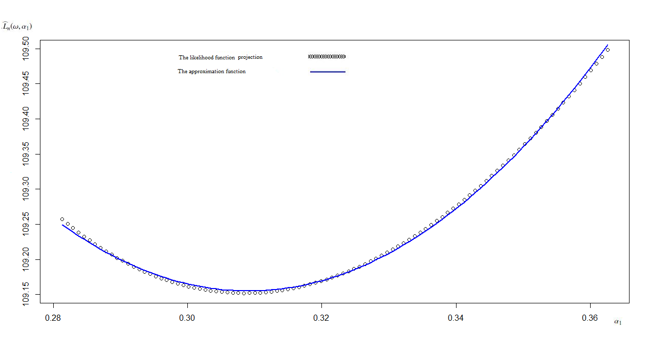 Figure 1
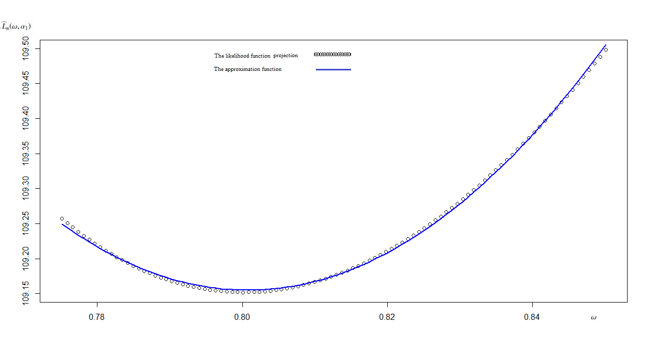 Figure 2
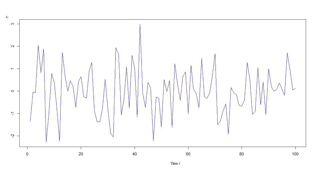 Figure 3
| Time | 1 | 2 | 3 | 4 | 5 | 6 | 7 | 8 | 9 | 10 |
|---|---|---|---|---|---|---|---|---|---|---|
| -1.348 | -0.05 | -0.063 | 2.055 | 0.815 | 1.893 | -2.277 | -1 | 0.782 | 0.351 | |
| Time | 11 | 12 | 13 | 14 | 15 | 16 | 17 | 18 | 19 | 20 |
| -0.791 | -2.24 | 1.723 | 0.667 | -0.015 | 0.464 | 0.22 | -0.737 | 0.434 | 0.643 | |
| Time | 21 | 22 | 23 | 24 | 25 | 26 | 27 | 28 | 29 | 30 |
| -0.259 | -0.313 | 0.907 | 1.268 | -0.888 | -1.376 | -1.367 | -0.805 | 0.528 | -0.813 | |
| Time | 31 | 32 | 33 | 34 | 35 | 36 | 37 | 38 | 39 | 40 |
| -1.89 | -2.051 | 1.94 | 1.643 | -1.071 | -0.336 | 1.085 | -0.766 | 1.59 | 0.993 | |
| Time | 41 | 42 | 43 | 44 | 45 | 46 | 47 | 48 | 49 | 50 |
| -1.162 | 2.985 | -0.1 | -0.732 | 0.391 | 0.132 | -2.224 | -0.271 | -0.336 | -1.606 | |
| Time | 51 | 52 | 53 | 54 | 55 | 56 | 57 | 58 | 59 | 60 |
| 0.509 | -0.026 | 0.468 | -1.626 | 1.219 | 0.315 | -0.416 | 0.636 | 0.848 | -1.011 | |
| Time | 61 | 62 | 63 | 64 | 65 | 66 | 67 | 68 | 69 | 70 |
| 1.152 | 0.085 | -0.114 | -0.744 | 1.456 | -0.243 | -0.332 | -0.078 | 0.678 | 1.668 | |
| Time | 71 | 72 | 73 | 74 | 75 | 76 | 77 | 78 | 79 | 80 |
| -1.499 | -1.347 | -0.886 | -0.578 | -1.94 | 0.156 | -0.082 | -0.173 | -0.63 | -0.677 | |
| Time | 81 | 82 | 83 | 84 | 85 | 86 | 87 | 88 | 89 | 90 |
| -0.397 | 1.283 | 0.479 | -1.035 | -0.917 | 1.054 | -0.605 | 0.412 | -1.055 | 0.994 | |
| Time | 91 | 92 | 93 | 94 | 95 | 96 | 97 | 98 | 99 | 100 |
| -0.259 | -0.313 | 0.907 | 1.268 | -0.888 | -1.376 | -1.367 | -0.805 | 0.528 | -0.813 |
| 0.0001 | 0.2001 | 0.4001 | 0.6001 | 0.8001 | |
| -7613853 | -455.4789 | -93.72643 | -19.2947 | 5.967303 |
| 0.7751 | 0.7759 | 0.7766 | 0.7774 | 0.7781 | 0.7789 | 0.7796 | 0.7804 | 0.7812 | 0.7819 | |
| 0.2813 | 0.2821 | 0.283 | 0.2838 | 0.2846 | 0.2854 | 0.2862 | 0.2871 | 0.2879 | 0.2887 | |
| 109.257 | 109.251 | 109.245 | 109.239 | 109.233 | 109.227 | 109.222 | 109.217 | 109.212 | 109.207 | |
| 0.7827 | 0.7834 | 0.7842 | 0.7849 | 0.7857 | 0.7865 | 0.7872 | 0.788 | 0.7887 | 0.7895 | |
| 0.2895 | 0.2903 | 0.2912 | 0.292 | 0.2928 | 0.2936 | 0.2945 | 0.2953 | 0.2961 | 0.2969 | |
| 109.202 | 109.198 | 109.194 | 109.19 | 109.186 | 109.182 | 109.179 | 109.176 | 109.173 | 109.17 | |
| 0.7903 | 0.791 | 0.7918 | 0.7925 | 0.7933 | 0.794 | 0.7948 | 0.7956 | 0.7963 | 0.7971 | |
| 0.2977 | 0.2986 | 0.2994 | 0.3002 | 0.301 | 0.3018 | 0.3027 | 0.3035 | 0.3043 | 0.3051 | |
| 109.168 | 109.165 | 109.163 | 109.161 | 109.159 | 109.158 | 109.156 | 109.155 | 109.154 | 109.153 | |
| 0.7978 | 0.7986 | 0.7993 | 0.8001 | 0.8009 | 0.8016 | 0.8024 | 0.8031 | 0.8039 | 0.8046 | |
| 0.3059 | 0.3068 | 0.3076 | 0.3084 | 0.3092 | 0.3100 | 0.3109 | 0.3117 | 0.3125 | 0.3133 | |
| 109.153 | 109.152 | 109.152 | 109.152 | 109.152 | 109.152 | 109.153 | 109.153 | 109.154 | 109.155 | |
| 0.8054 | 0.8062 | 0.8069 | 0.8077 | 0.8084 | 0.8092 | 0.8099 | 0.8107 | 0.8115 | 0.8122 | |
| 0.3141 | 0.315 | 0.3158 | 0.3166 | 0.3174 | 0.3183 | 0.3191 | 0.3199 | 0.3207 | 0.3215 | |
| 109.156 | 109.157 | 109.159 | 109.161 | 109.162 | 109.164 | 109.167 | 109.169 | 109.171 | 109.174 | |
| 0.813 | 0.8137 | 0.8145 | 0.8153 | 0.816 | 0.8168 | 0.8175 | 0.8183 | 0.819 | 0.8198 | |
| 0.3224 | 0.3232 | 0.324 | 0.3248 | 0.3256 | 0.3265 | 0.3273 | 0.3281 | 0.3289 | 0.3297 | |
| 109.177 | 109.18 | 109.183 | 109.186 | 109.19 | 109.193 | 109.197 | 109.201 | 109.205 | 109.21 | |
| 0.8206 | 0.8213 | 0.8221 | 0.8228 | 0.8236 | 0.8243 | 0.8251 | 0.8259 | 0.8266 | 0.8274 | |
| 0.3306 | 0.3314 | 0.3322 | 0.333 | 0.3338 | 0.3347 | 0.3355 | 0.3363 | 0.3371 | 0.3379 | |
| 109.214 | 109.218 | 109.223 | 109.228 | 109.233 | 109.238 | 109.244 | 109.249 | 109.255 | 109.26 | |
| 0.8281 | 0.8289 | 0.8296 | 0.8304 | 0.8312 | 0.8319 | 0.8327 | 0.8334 | 0.8342 | 0.8349 | |
| 0.3388 | 0.3396 | 0.3404 | 0.3412 | 0.3421 | 0.3429 | 0.3437 | 0.3445 | 0.3453 | 0.3462 | |
| 109.266 | 109.272 | 109.279 | 109.285 | 109.291 | 109.298 | 109.305 | 109.312 | 109.319 | 109.326 | |
| 0.8357 | 0.8365 | 0.8372 | 0.838 | 0.8387 | 0.8395 | 0.8403 | 0.841 | 0.8418 | 0.8425 | |
| 0.347 | 0.3478 | 0.3486 | 0.3494 | 0.3503 | 0.3511 | 0.3519 | 0.3527 | 0.3535 | 0.3544 | |
| 109.333 | 109.341 | 109.349 | 109.356 | 109.364 | 109.372 | 109.38 | 109.389 | 109.397 | 109.406 | |
| 0.8433 | 0.844 | 0.8448 | 0.8456 | 0.8463 | 0.8471 | 0.8478 | 0.8486 | 0.8493 | 0.8501 | |
| 0.3552 | 0.356 | 0.3568 | 0.3576 | 0.3585 | 0.3593 | 0.3601 | 0.3609 | 0.3617 | 0.3626 | |
| 109.414 | 109.423 | 109.432 | 109.441 | 109.45 | 109.46 | 109.469 | 109.479 | 109.488 | 109.498 |
| Sample size | Our Method | BGFS | Simplex | OPR | Our Method | BGFS | Simplex | OPR | |
|---|---|---|---|---|---|---|---|---|---|
| 100 | 0.485 | 0.607 | 0.609 | 0.609 | 0.798 | 0.804 | 0.807 | 0.807 | |
| 200 | 0.345 | 0.368 | 0.368 | 0.368 | 0.747 | 0.752 | 0.752 | 0.752 | |
| 300 | 0.292 | 0.300 | 0.300 | 0.300 | 0.742 | 0.743 | 0.743 | 0.743 | |
Peer Reviews
No public reviews on file for this paper yet. If you reviewed it on a platform where reviews are public (OpenReview, ICLR, NeurIPS, ICML), you can paste yours below so the community can read it here.
Videos
No videos yet. Explain this paper in a talk, walkthrough, or lecture? Add one.
Taxonomy
TopicsImage and Signal Denoising Methods · Financial Risk and Volatility Modeling · Hydrology and Drought Analysis
New approximation for GARCH parameters estimate
Yakoub BOULAROUK1 , Nasr-eddine HAMRI1
1 Institute of Science and Technology, Melilab laboratory, University Center of Mila, Algeria
Abstract: This paper presents a new approach for the optimization of GARCH parameters estimation. Firstly, we propose a method for the localization of the maximum. Thereafter, using the methods of least squares, we make a local approximation for the projection of the likelihood function curve on two dimensional planes by a polynomial of order two which will be used to calculate an estimation of the maximum.
Keyword GARCH Process, Likelihood function, Least squares.
1 Introduction
The modeling of time series is applied today in fields as diverse (econometrics, medicine or demographics….). As it is a crucial step in the study of time series, it has undergone a great evolution during the last fifty years and several models of representation have been proposed.
In 1982, Engle [4] proposed the conditionally heteroskedastic autoregressive (ARCH) model, which allowed the conditional variance to change as a function of past errors over time, while leaving the variance unconditional constant. This model has already proved useful in the modeling of several phenomenas. In Engle [4, 5] and Engle and Kraft [6], models for the inflation rate are constructed recognizing that the uncertainty of inflation tends to change over time. In 1984, Weiss [14] considered the ARMA models with ARCH errors. He used these models for the modeling of sixteen US microeconomic time series.
In 1986, Bollerslev [1] proposed a generalization of these ARCH models to the Generalized AutoRegressive Conditional Heteroskedasticity (GARCH) models, whose the variance in the present depends on its past and the process past. As it studied the conditions of stationarity and the structure of the autocorrelations for this class of models.
The GARCH family contains a number of parameters which must be estimated on actual data for empirical applications. The estimation of the parameters returns to calculate the maximum of the log-likelihood function which is non-linear, this leads to the use of non-linear optimization methods. Several optimization methods are used, including The Nelder-Mead method, BGFS method and others :
- •
Nelder and Mead [11] introduced their method using only
the likelihood function values. Altough their method is relatively slow, it’s robust and leads to results for the non differentiable functions. In their turn Fletcher and Reeves [9] have introduced the method of the conjugate gradient which does not store matrix.
- •
In 1970 Broyden [3], Fletcher [8], Goldfarb [10] and Shanno [12] have published simultaneously the method entitled quasi-Newton (noted BFGS), which uses the values and the gradients of function to construct an image of the surface to optimize.
- •
In 1990 David M. Gay [7] have published a technical report in which he proposed a method intitiled optimization using PORT routines (noted OPR).
It is common knowledge among practitioners that the GARCH parameters are numerically difficult to estimate in empirical applications. The existant numerical algorithm can easily fail, or converge to erratic solutions. Therefore, the resulting fitted parameters must be examined with a healthy dose of scepticism. In this work, we propose a new algorithm in which we exploit the asymptotic convexity of the likelihood function. We will develop a method to locate the maximum value instead of using the confidence intervals resulting from asymptotic normality of the estimated parameters thereafter and as in [2], we approach the likelihood function by a quadratic form that we use to calculate an approximation of the maximum.
2 The GARCH model and its likelihood function
The GARCH process was introduced by Bollerslev [1] as solution for the system of equations:
[TABLE]
Let’s note the vector of unknown parameters, with , for , for , strictly positive. The is a sequence of normal random independent and identically distributed satisfying the standard assumptions and . The ARCH is an GARCH
The conditional likelihood of expresses as, up to an additional constant,
[TABLE]
The quasi-likelihood is obtained by plugging in the approximations , where is different of zero only for finitely many ,
[TABLE]
Remark that unobserved values have to be fixed a priori equal to in the quasi-likelihood . In the next proposition, we give a necessary and sufficient condition for the process stationarity.
Proposition 2.1**.**
The GARCH( ) process as defined in (2.1) is wide-sense stationary with , and for if and only if
[TABLE]
Proof 1**.**
This result is proved by Bollerslev in [1].
The condition (2.2) implies that and .
Else, we define the stationarity set
[TABLE]
3 Necessary tools
3.1 Convexity
W.C. Ip and al. [13] have proved the convexity of the negative likelihood function in the asymptotic sense for GARCH models. This property allows us the local approximation of this function in the Neighborhood of its minimum by a polynomial of degree two.
Proposition 3.1**.**
Suppose is an arbitrary compact, convex subset of and the second derivative of . Then there exist a constant and a set with satisfying that for each and , there is a positive integer such that
[TABLE]
3.2 Localisation method
In this part, we propose a method to search for a block of the form containing the maximum sought-after. The method is based on the principle of dichotomy applied for projections of the likelihood function on a plane with dimension two, we follow the steps
We search a point that verifie , where is the order derivative of the likelihood function with respect to . 2. 2.
We put and 3. 3.
- •
if \widehat{L^{{}^{\prime}}_{i,n}}\big{(}\underline{\theta_{1}},...,\underline{\theta_{i}},....,\underline{\theta}_{p+q+1}\big{)}\widehat{L_{i,n}}^{{}^{\prime}}\big{(}\underline{\theta_{1}},....,(\underline{\theta}_{i}+\overline{\theta}_{i})/2,....,\underline{\theta}_{p+q+1}\big{)}<0 then we replace by
- •
else if \widehat{L^{{}^{\prime}}_{i,n}}\big{(}\underline{\theta_{1}},...,\underline{\theta_{i}},....,\underline{\theta_{p+q+1}}\big{)}\widehat{L_{i,n}}^{{}^{\prime}}\big{(}\underline{\theta_{1}},....,(\underline{\theta}_{i}+\overline{\theta}_{i})/2,....,\underline{\theta}_{p+q+1}\big{)}>0 we replace by
We repeat the step until .
4 Calculation procedure
To calculate the maximum likelihood, one passes by the following steps
Calculate confidence intervals for the unknown parameters using the localisation method. 2. 2.
Make a subdivision of elements for all the confidence intervals . 3. 3.
Calculate the function values \big{[}l_{n}(\theta_{j})\big{]}_{j=1,m} where , Which is a cut for the curve of the likelihood function on the diagonal plane of the confidence region. 4. 4.
Numerical approximation for the orthogonal projection of the log likelihood function cut by polynomials of order two taking the form : we use the least squares method. 5. 5.
Calculate these maximum.
5 Example of application ARCH(1)
The process is presented as solution of the system
[TABLE]
where and .
Let be the simulated first order conditionally heteroskedastic autoregressive time series with ( and ) presented by the table 3.
We plot this time series as function of time
The log likelihood of an process is given by
[TABLE]
to obtain we replace by zero.
Now, we proceed to the calculation of the maximum likelihood using our method
We remark that , therefore .
Using the localisation procedure, we find that the region contains the maximum. 3. 3.
We calculate the function values on the diagonal plane of the confidence region, which give the table 3.
Using the least squares method, we calculate approximations of \big{(}\omega_{i},\widehat{L}_{n}(\omega_{i},\alpha_{1i})\big{)}_{i=1,100} and \big{(}\alpha_{1i},\widehat{L}_{n}(\omega_{i},\alpha_{1i})\big{)}_{i=1,100} the orthogonal projections of the likelihood function curve cut \big{(}\omega_{i},\alpha_{1i},\widehat{L}_{n}(\omega_{i},\alpha_{1i})\big{)}_{i=1,100} on the planes , respectively.
- •
The approximation function for the likelihood function Curve cut projection on the plane is
;
the maximum of this function is .
In the Figure 2, we represent the projection of the cut of the likelihood function on the plane and its approximation
- •
The approximation function for the likelihood function curve cut projection on the plane is
;
the maximum value of this function is .
The Figure 3 illustrates the projection of the cut of the likelihood function on the plane and its approximation
6 Numerical comparaison study
To illustrate the performance of the proposed method, we compare it with some popular methods (BGFS, Simplex and OPR) usually used in the Time series parameters calculation. We applied these methods to independent replications of two ARCH process (one with , end the other with , for different sample size , and , thereafter we compute the root-mean-square error (RMSE) of the resulting estimation, the results are presented in Table 4.
Conclusion of the numerical comparaison results: On the one hand, it is clear that the RMSE decreases as the sample size increases, which validates the theoretical results (consistency of the estimators). On the other hand, Table 4 show that our method provides more accurate estimation than the BGFS, Simplex and OPR methods.
The reference list from the paper itself. Each links out to its DOI / PubMed record.
- 1[1] Bollerslev, T. (1986), Generalised autoregressive conditional heteroscedasticity, Journal of Econometrics, 31, 307-327.
- 2[2] Y. Boularouk and K. Djeddour (2015), New approximation for ARMA parameters estimate, Mathematics and Computers in Simulation, 118,116-122.
- 3[3] Broyden, C. G. (1970), The convergence of a class of double-rank minimization algorithms, Journal of the Institute of Mathematics and Its Applications, 6, 76-90.
- 4[4] Engle, R.F. (1982), Autoregressive conditional heteroskedasticity with estimates of the variance of U.K. inflation, Econometrica 50, 987-1008.
- 5[5] Engle, R.F. (1983), Estimates of the variance of U.S. inflation based on the ARCH model, Journal of Money Credit and Banking 15, 286-301.
- 6[6] Engle, R.F. and D. Kraft (1983), Multiperiod forecast error variances of inflation estimated from ARCH models, in: A. Ze Uner, ed., Applied time series analysis of economic data (Bureau of the Census, Washington, DC) 293-302.
- 7[7] David M. Gay (1990), Usage summary for selected optimization routines. Computing Science Technical Report 153, AT and T Bell Laboratories, Murray Hill.
- 8[8] Fletcher, R. (1970), A New Approach to Variable Metric Algorithms, Computer Journal, 13, 3, 317-322