Stability analysis of LPV systems with piecewise differentiable parameters
Corentin Briat, Mustafa Khammash

TL;DR
This paper introduces a hybrid systems approach to analyze the stability of LPV systems with piecewise differentiable parameters, unifying existing criteria and providing tractable conditions via sum of squares programming.
Contribution
It proposes a novel hybrid systems framework for LPV stability analysis, generalizing quadratic and robust criteria with finite-dimensional relaxations.
Findings
Unified stability conditions for LPV systems with piecewise differentiable parameters.
Relaxation via sum of squares programming yields practical stability tests.
Illustrated effectiveness on literature examples.
Abstract
Linear Parameter-Varying (LPV) systems with piecewise differentiable parameters is a class of LPV systems for which no proper analysis conditions have been obtained so far. To fill this gap, we propose an approach based on the theory of hybrid systems. The underlying idea is to reformulate the considered LPV system as an equivalent hybrid system that will incorporate, through a suitable state augmentation, information on both the dynamics of the state of the system and the considered class of parameter trajectories. Then, using a result pertaining on the stability of hybrid systems, two stability conditions are established and shown to naturally generalize and unify the well-known quadratic and robust stability criteria together. The obtained conditions being infinite-dimensional, a relaxation approach based on sum of squares programming is used in order to obtain tractable…
Click any figure to enlarge with its caption.
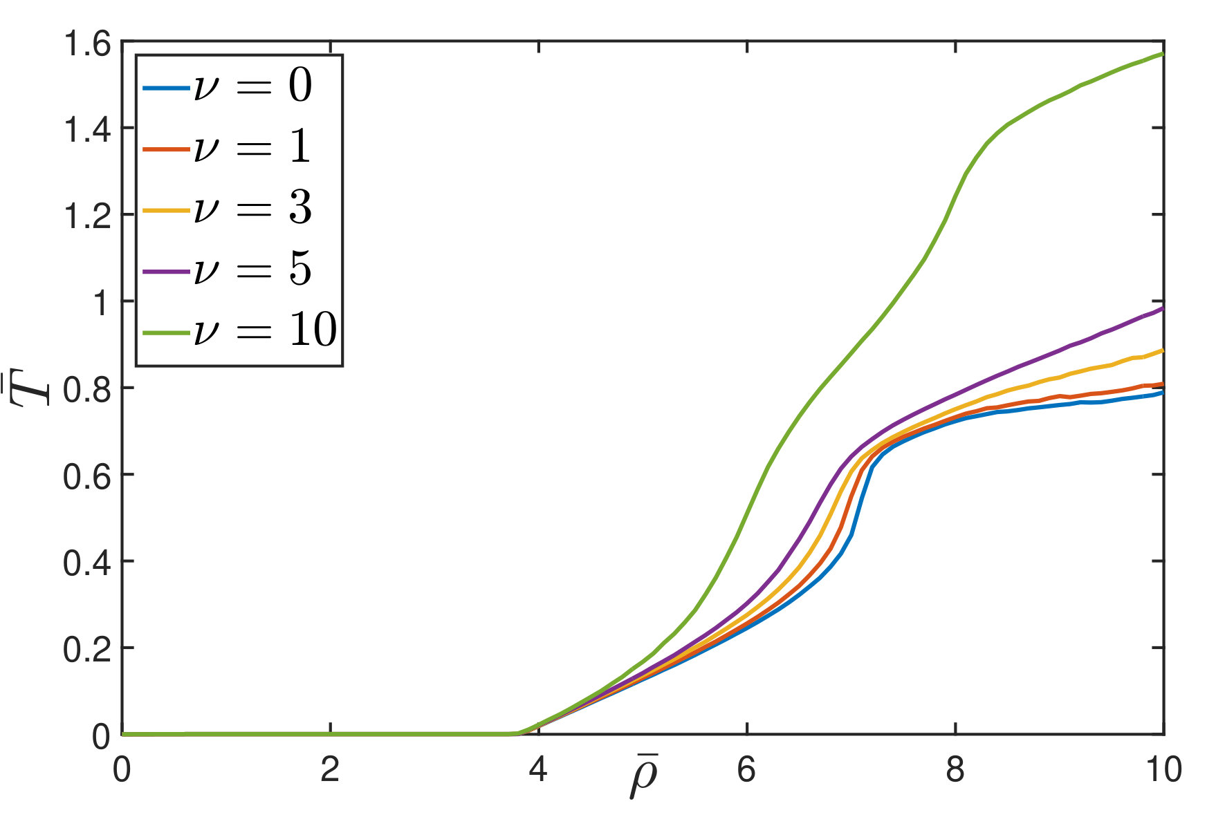 Figure 1
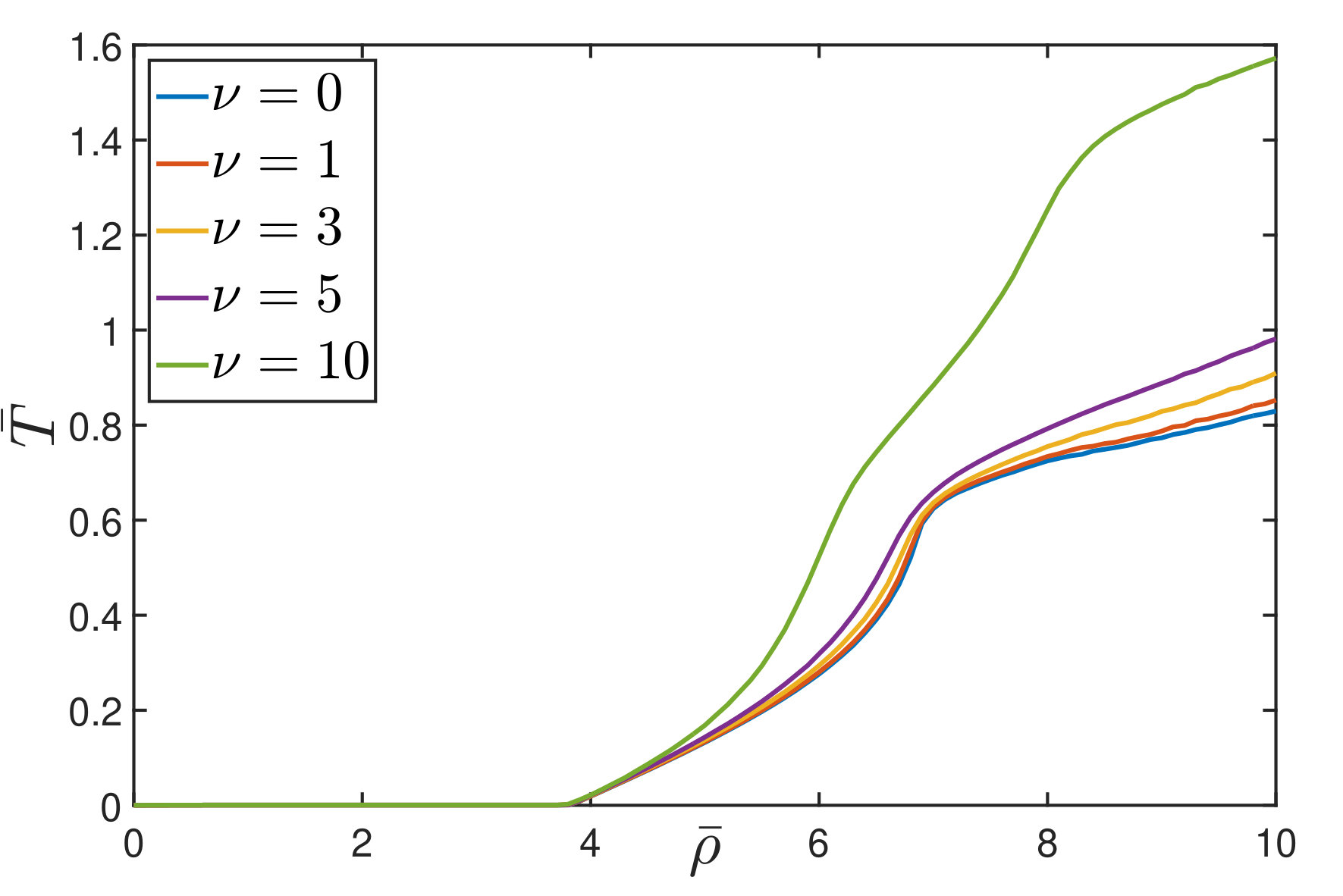 Figure 2
| primal/dual vars. | time (sec) | |||||||
|---|---|---|---|---|---|---|---|---|
| 2.7282 | 2.9494 | 3.5578 | 4.6317 | 11.6859 | 26.1883 | 9820/1850 | 20/27 | |
| 1.7605 | 1.8881 | 2.2561 | 2.9466 | 6.4539 | num. err. | 43300/4620 | 212/935 |
Peer Reviews
No public reviews on file for this paper yet. If you reviewed it on a platform where reviews are public (OpenReview, ICLR, NeurIPS, ICML), you can paste yours below so the community can read it here.
Videos
No videos yet. Explain this paper in a talk, walkthrough, or lecture? Add one.
Stability analysis of LPV systems with piecewise differentiable parameters
Corentin Briat and Mustafa Khammash Corentin Briat and Mustafa Khammash are with the Department of Biosystems Science and Engineering, ETH-Zürich, Switzerland; email: [email protected], [email protected], [email protected]; url: https://www.bsse.ethz.ch/ctsb/, http://www.briat.info.
Abstract
Linear Parameter-Varying (LPV) systems with piecewise differentiable parameters is a class of LPV systems for which no proper analysis conditions have been obtained so far. To fill this gap, we propose an approach based on the theory of hybrid systems. The underlying idea is to reformulate the considered LPV system as an equivalent hybrid system that will incorporate, through a suitable state augmentation, information on both the dynamics of the state of the system and the considered class of parameter trajectories. Then, using a result pertaining on the stability of hybrid systems, two stability conditions are established and shown to naturally generalize and unify the well-known quadratic and robust stability criteria together. The obtained conditions being infinite-dimensional, a relaxation approach based on sum of squares programming is used in order to obtain tractable finite-dimensional conditions. The approach is finally illustrated on two examples from the literature.
1 Introduction
Linear Parameter-Varying (LPV) systems [1, 2, 3] are an important class of linear systems that can be used to model linear systems that intrinsically depend on parameters [4] or to approximate nonlinear systems in the objective of designing gain-scheduled controllers [5, 6]; see [3] for a classification attempt. They have been, since then, successfully applied to a wide variety of real-world systems such as automotive suspensions systems [7, 8], robotics [9], aperiodic sampled-data systems [10], aircrafts [11, 12, 13], etc. The field has also been enriched with very broad theoretical results and numerical tools [14, 15, 16, 17, 18, 19, 20, 21, 22, 23, 3, 24, 25, 26, 27].
The objective of the paper is to extend the stability results in [24] for LPV systems with piecewise constant parameters to the case of piecewise differentiable parameters. Such parameter trajectories may arise whenever an (impulsive) LPV system is used to approximate a nonlinear impulsive system or in linear systems where parameters naturally have such a behavior. Finally, they can also be used to approximate parameter trajectories that exhibit intermittent very fast, yet differentiable, variations. Despite being similar to the case of piecewise constant parameters, the fact that the parameters are time-varying between discontinuities leads to additional difficulties which prevent from straightforwardly extending the approach developed in [24]. To overcome this, we propose a different, more general, approach based on hybrid systems theory [28]. Firstly, we equivalently reformulate the considered LPV system into a hybrid system that captures in its formulation both the dynamics of the state of the system and the considered class of parameter trajectories. Recent results from hybrid systems theory [28] combined with the use of quadratic Lyapunov functions are then applied in order to derive sufficient stability conditions for the considered hybrid systems and, hence, for the associated LPV system and class of parameter trajectories. We then prove that the obtained stability conditions generalize and unify the well-known quadratic stability and robust stability conditions, which can be recovered as extremal/particular cases. The obtained infinite-dimensional stability conditions are reminiscent of those obtained in [29, 30, 31], a fact that strongly confirms the connection between the approaches. To make these conditions computationally verifiable, we propose a relaxation approach based on sum of squares [32, 33, 34] and semidefinite programming [35]. The approach is finally validated through two examples.
Outline. The structure of the paper is as follows: in Section 2 preliminary definitions and results are given. Section 3 develops the main results of the paper. Examples are finally given in Section 4.
Notations. The set of nonnegative integers is denoted by . The set of symmetric matrices of dimension is denoted by while the cone of positive (semi)definite matrices of dimension is denoted by () . For some , the notation that means that is positive (semi)definite. The maximum and the minimum eigenvalue of a symmetric matrix are denoted by and , respectively. A function is of class (i.e. ), if it is continuous, zero at zero, increasing and unbounded. A function is positive definite if for all and . Given a vector and a closed set , the distance of to the set is denoted by and is defined by . For any differentiable function , the partial derivatives with respect to the first and second argument evaluated at are denoted by and , respectively.
2 Preliminaries
2.1 LPV systems
LPV systems are dynamical systems that can be described as
[TABLE]
where are the state of the system and the initial condition, respectively. The matrix-valued function is assumed to be bounded and continuous. The parameter vector trajectory , compact and connected, is assumed to be piecewise differentiable with derivative in , where is also compact and connected. When the parameters are independent of each other, then we can assume that is a box and that the following decompositions hold where , and where , . We also define the set of vertices of as ; i.e. .
2.2 Hybrid systems
Let us consider here the following hybrid system
[TABLE]
where , is open, is compact and . The flow map and the jump map are the set-valued maps and , respectively. Note that the trajectories of the above system are left-continuous and the right-handed limit is given denoted by . It is often convenient to define a solution (or hybrid arc) to the above system over a hybrid time domain where the first component denotes the usual continuous-time while the second one counts the number of jumps111See [28] for more details about the solutions of (2).. We also assume for simplicity that the solutions are complete (i.e. is unbounded). We then have the following stability result:
Theorem 1** ([28])**
Let be closed. Assume that there exist a function that is continuously differentiable on an open set containing (i.e. the closure of ), functions and a continuous positive definite function such that
- (a)
* for all ;* 2. (b)
* for all and ;* 3. (c)
* for all and .*
Assume further that for each , there exists a and an such that for every solution to the system (2), we have that , , imply , then is uniformly globally asymptotically stable for the system (2).
The above stability result only requires the flow part of the system to be stabilizing while the jump part is only required to be non-expansive. This result is fully adapted to the analysis of LPV systems with piecewise differentiable parameters since discontinuous changes in the values of the parameters can not have any stabilizing effect – quite the opposite. In this regard, the asymptotic stability of the system can only be ensured by the flow part of the system where parameters are smoothly varying.
3 Main results
The objective of this section is to present the main results on the paper: the stability problem in the case of periodic parameter discontinuities is addressed in Section 3.1 and extended to the aperiodic case in Section 3.2. The results are connected to existing ones in Section 3.3. Finally, some computational discussions are provided in Section 3.4.
3.1 Stability under constant dwell-time
In this section, we will consider the family of piecewise differentiable parameter trajectories given by
[TABLE]
where , , and with
[TABLE]
In other words, the trajectories contained in this family can only exhibit jumps at the times , (we assume that no discontinuity occurs at ) and hence the distance between two potential successive discontinuities – the so-called dwell-time – is given by and is constant, whence the name constant dwell-time. The associated hybrid system is given by
[TABLE]
where
[TABLE]
The initial condition for this system is chosen such that . Note, moreover, that , and . Hence, starting from the above initial condition, the solution of the hybrid system (5) is complete (i.e. it is defined for all ) and it is confined in .
The above hybrid system interestingly incorporates both the dynamics of the state of the system and the considered class of parameter trajectories. In addition to that, the state is also augmented to contain a clock that will measure the time elapsed since the last jump in the parameter trajectories. Indeed, starting from the chosen initial condition, the system will smoothly flow until the clock reaches the value upon which the jump map is activated. The jump map changes the value of the parameter (thereby introducing a discontinuity in the parameter trajectories) and resets the clock, which places back the system in flow-mode. In this regard, we can easily observe that this formulation incorporates all the necessary information about the system and the parameter trajectories in order to provide accurate stability results. Such a result based on the use of a quadratic Lyapunov function is given below:
Theorem 2** (Constant dwell-time)**
Let be given and assume that there exist a bounded continuously differentiable matrix-valued function and a scalar such that the conditions
[TABLE]
and
[TABLE]
hold for all , all and all .
Then the LPV system (1) with parameter trajectories in is asymptotically stable.
*Proof : * Let and note that the LPV system (1) with parameter trajectories in is asymptotically stable if and only if is asymptotically stable for the system (5). We prove now that for the choice of the Lyapunov function with for all and all , the feasibility of the conditions of Theorem 2 implies the feasibility of those in Theorem 1.
Since for all and all , then if and only if and, hence, the conditions of statement (a) of Theorem 1 are verified with the functions
[TABLE]
which are both functions.
To prove that the feasibility of the condition (7) implies that of statement (b) of Theorem 1, let be the matrix on the left-hand side of (7) when . Using the linearity in , it is immediate to get that for all if and only if for all . Hence, (7) is equivalent to saying that
[TABLE]
for all . Therefore, we have that the feasibility of the condition (7) implies that of statement (b) of Theorem 1 with , which is positive definite.
Finally, the condition of statement (c) reads
[TABLE]
and must hold for all . This is equivalent to the condition (8). Finally, we need to check the time-domain condition. First, note that
[TABLE]
which, together with for some , implies that since for all . Hence, and, as a result, the set is asymptotically stable for the system (5) and the result follows.
3.2 Stability under minimum dwell-time
Let us consider now the family of piecewise differentiable parameter trajectories given by
[TABLE]
where , (we again assume that no discontinuity can occur at ). The corresponding hybrid system is given by
[TABLE]
where
[TABLE]
The initial condition for this system is chosen such that . This system contains an additional state compared to the system considered in Section 3.1 in order to avoid the use of a time-dependent jump set (a purely technical requirement that can be relaxed). Using the current formulation, the current dwell-time is drawn each time the system jumps and the jumping condition is satisfied when . This leads to the following result:
Theorem 3** (Minimum dwell-time)**
Let be given and assume that there exist a bounded continuously differentiable matrix-valued function and a scalar such that the conditions
[TABLE]
[TABLE]
and
[TABLE]
hold for all , and all . Then, the LPV system (1) with parameter trajectories in is asymptotically stable.
*Proof : * Assume that the full trajectory of is known and such that for all . Note that this is possible since is independent of the rest of the state of the hybrid system (14). Then, there exists a such that for all and define the set . Let us consider here the following Lyapunov function
[TABLE]
The rest of the proof is analogous to that of Theorem 2 and it thus omitted.
3.3 Connection with quadratic and robust stability
Interestingly, it can be shown that the minimum dwell-time result stated in Theorem 3 naturally generalizes and unifies the quadratic and robust stability conditions through the concept of minimum dwell-time. This is further explained in the results below:
Proposition 4** (Quadratic stability)**
When and as , then the conditions of Theorem 3 are equivalent to saying that there exists a matrix such that
[TABLE]
for all .
*Proof : * First note that since and as , then the solution of the hybrid system is complete. Let , then we have that
[TABLE]
where it is assumed that and where is the little-o notation. From (18), we get that the first equation implies that . Therefore, for the second expression to be negative semidefinite for any arbitrarily small , we need that be negative semidefinite. However, this contradicts the last one and hence we need that ; i.e. is independent of . Finally, since is arbitrarily small, then both (16)-(17) can be satisfied with a matrix-valued function that is independent of . Hence, we need that and substituting it in (16)-(17) yield the quadratic stability condition (20).
Proposition 5** (Robust stability)**
When , then the conditions of Theorem 3 are equivalent to saying that there exists a differentiable matrix-valued function such that
[TABLE]
for all and all .
*Proof : * Clearly, when , then there are no jumps anymore and hence we can remove the condition (18) as it never occurs. Consequently, we can choose and the conditions (16)-(17) immediately reduce to (22).
3.4 Computational considerations
The conditions formulated in Theorem 2 and Theorem 3 are infinite-dimensional semidefinite programs that are intractable per se. To make them tractable, we propose to consider an approach based on sum of squares programming [33] that will result in a approximate finite-dimensional semidefinite program that can be solved using standard semidefinite programming solvers such as SeDuMi [35]. The relaxation procedure can be performed with the help of the package SOSTOOLS [34] This conversion to an SOS program is described below.
Assuming that is a compact semialgebraic set, then it can defined as
[TABLE]
where the functions , are polynomial. We further have that
[TABLE]
In what follows, we say that a symmetric matrix-valued function is a sum of squares matrix (SOS matrix) if there exists a matrix such that . The following result provides the sum of squares formulation of Theorem 2:
Proposition 6
Let be given and assume that the sum of squares program
Find polynomial matrices
\begin{array}[]{rcl}S,\Gamma_{1},\Gamma_{2},\Gamma_{1}^{i},\Gamma_{2}^{i}&:&[0,\bar{T}]\times\mathcal{P}\mapsto\mathbb{S}^{n},\\ \Gamma_{3}^{i},\Gamma_{4}^{i}&:&\mathcal{P}\times\mathcal{P}\mapsto\mathbb{S}^{n},\\ \Upsilon_{1}^{i},\Upsilon_{2}^{i}&:&\mathcal{D}^{v}\times[0,\bar{T}]\times\mathcal{P}\mapsto\mathbb{S}^{n}\end{array}
where and such that
•
, , are SOS matrices for all ,
•
* is an SOS matrix*
•
**
* is an SOS matrix for all *
•
* is an SOS matrix.*
**
is feasible. Then, the conditions of Theorem 2 hold with the computed polynomial matrix and the system (1) is asymptotically stable for all .
Remark 7
The conditions of Theorem 3 can be checked by simply adding to the SOS program of Proposition 6 the constraints
- •
, , are SOS matrices for all
- •
* is an SOS matrix for all *
where , , are additional polynomial variables.
Remark 8
When the parameter set is also defined by equality constraints , , these constraints can be simply added in the sum of squares programs in the same way as the inequality constraints, but with the particularity that the corresponding multiplier matrices be simply symmetric instead of being symmetric SOS.
4 Examples
We consider now two examples. The first one is a 2-dimensional toy example considered in [36] whereas the second one is a 4-dimensional system considered in [4] and inspired from an automatic flight control design problem.
4.1 Example 1
Let us consider the system (1) with the matrix [36, 24]
[TABLE]
where the time-varying parameter takes values in , . It is known [36] that this system is quadratically stable if and only if but it is was later proven in the context of piecewise constant parameters [24] that this bound can be improved provided that discontinuities do not occur too often. We now apply the conditions of Theorem 2 and Theorem 3 in order to characterize the impact of parameter variations between discontinuities. To this aim, we consider that with and that . For each value for the upper-bound in that set, we solve for the conditions Theorem 2 and Theorem 3 to get estimates (i.e. upper-bounds) for the minimum stability-preserving constant and minimum dwell-time. We use here and polynomials of degree 4 in the sum of squares programs. Note that we have, in this case, , and . The complexity of the approach can be evaluated here through the number of primal/dual variables of the semidefinite program which is 2209/273 in the constant dwell-time case and 2409/315 in the minimum dwell-time case. Time-wise, the average preprocessing/solving time is given by 4.83/0.89 sec in the constant dwell-time case and 6.04/1.25 sec in the minimum dwell-time case. The results are depicted in Fig. 1 and Fig. 2 where we can see that the obtained minimum values for the dwell-times increase with the rate of variation of the parameter, which is an indicator of the fact that increasing the rate of variation of the parameter destabilizes the system and, consequently, the dwell-time needs to increase in order to preserve the overall stability of the system. For this example, it is interesting to note that the constant and minimum dwell-time curves seem to converge to each other when increases which could indicate that when the parameter is fast-varying between jumps then the aperiodicity of jumps do not affect much the stability of the system.
4.2 Example 2
Let us consider now the system (1) with the matrix considered in [4, p. 55]:
[TABLE]
where and . It has been shown in [4] that this system is not quadratically stable but was proven to be stable under minimum dwell-time equal to 1.7605 when the parameter trajectories are piecewise constant [24]. We propose now to quantify the effects of smooth parameter variations between discontinuities. Note, however, that the set is not a box as considered along the paper but the next calculations show that this is not a problem since a proper set for the values of the derivative of the parameters can be defined. To this aim, let us define the parametrization and where is piecewise differentiable. Differentiating these equalities yields and where , , at all times where is differentiable. In this regard, we can consider as an additional parameter that enters linearly in the stability conditions and hence the conditions can be checked at the vertices of the interval, that is, for all . Note that, in this case, we have , and .
We now consider the conditions of Theorem 3 and we get the results gathered in Table 1 where we can see that, as expected, when increases then the minimum dwell-time has to increase to preserve stability. Using polynomials of higher degree allows to improve the numerical results at the expense of an increase of the computational complexity. As a final comment, it seems important to point out the failure of the semidefinite solver due to too important numerical errors when and .
5 Conclusion
Reformulating LPV systems into hybrid systems enabled the derivation of tractable conditions for establishing the stability of LPV systems with piecewise differentiable parameters. These results extend those obtained in [24] for piecewise constant parameters through the use of a different, yet connected, approach. It is shown that the obtained stability conditions generalize and unify the well-known quadratic and robust stability conditions in a single formulation. Possible extensions include controller/filter/observer design and performance analysis.
The reference list from the paper itself. Each links out to its DOI / PubMed record.
- 1[1] R. Tóth. Modeling and Identification of Linear Parameter-Varying Systems . Springer, Germany, 2010.
- 2[2] J. Mohammadpour and C. W. Scherer, editors. Control of Linear Parameter Varying Systems with Applications . Springer, New York, USA, 2012.
- 3[3] C. Briat. Linear Parameter-Varying and Time-Delay Systems – Analysis, Observation, Filtering & Control , volume 3 of Advances on Delays and Dynamics . Springer-Verlag, Heidelberg, Germany, 2015.
- 4[4] F. Wu. Control of linear parameter varying systems . Ph D thesis, University of California Berkeley, 1995.
- 5[5] J. S. Shamma. Analysis and design of gain-scheduled control systems . Ph D thesis, Laboratory for Information and decision systems - Massachusetts Institute of Technology, 1988.
- 6[6] J. S. Shamma and M. Athans. Gain scheduling: potential hazards and possible remedies. IEEE Contr. Syst. Magazine , 12(3):101–107, 1992.
- 7[7] C. Poussot-Vassal, O. Sename, L. Dugard, P. Gáspár, Z. Szabó, and J. Bokor. New semi-active suspension control strategy through LPV technique. Control Engineering Practice , 2008.
- 8[8] S. M. Savaresi, C. Poussot-Vassal, C. Spelta, O. Sename, and L. Dugard. Semi-Active Suspension Control Design for Vehicles . Butterworth Heinemann, 2010.