Polynomial Profits in Renewable Resources Management
Rinaldo M. Colombo, Mauro Garavello

TL;DR
This paper develops a mathematical framework using renewal equations on graphs to optimize biological resource exploitation, proving the existence of optimal controls and characterizing their structure, including conditions for bang-bang solutions.
Contribution
It introduces a novel polynomial cost function approach in renewable resource management and provides conditions for optimal control structures, including bang-bang controls.
Findings
Optimal control exists for the resource exploitation model.
Under certain conditions, the optimal control is bang-bang.
The polynomial dependence simplifies the computation of optimal controls.
Abstract
A system of renewal equations on a graph provides a framework to describe the exploitation of a biological resource. In this context, we formulate an optimal control problem, prove the existence of an optimal control and ensure that the target cost function is polynomial in the control. In specific situations, further information about the form of this dependence is obtained. As a consequence, in some cases the optimal control is proved to be necessarily bang--bang, in other cases the computations necessary to find the optimal control are significantly reduced.
Click any figure to enlarge with its caption.
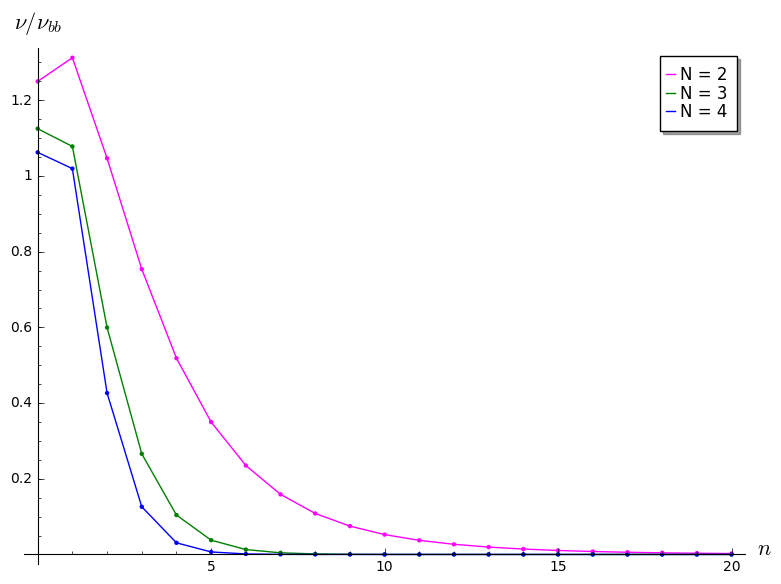 Figure 1
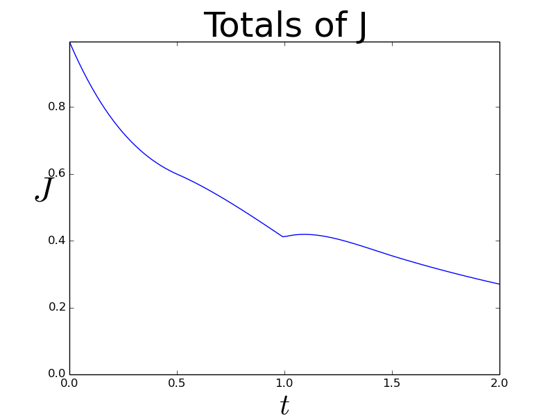 Figure 2
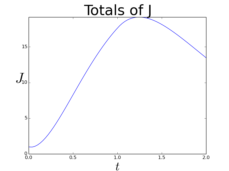 Figure 3
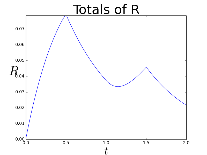 Figure 4
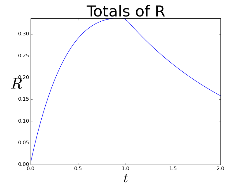 Figure 5
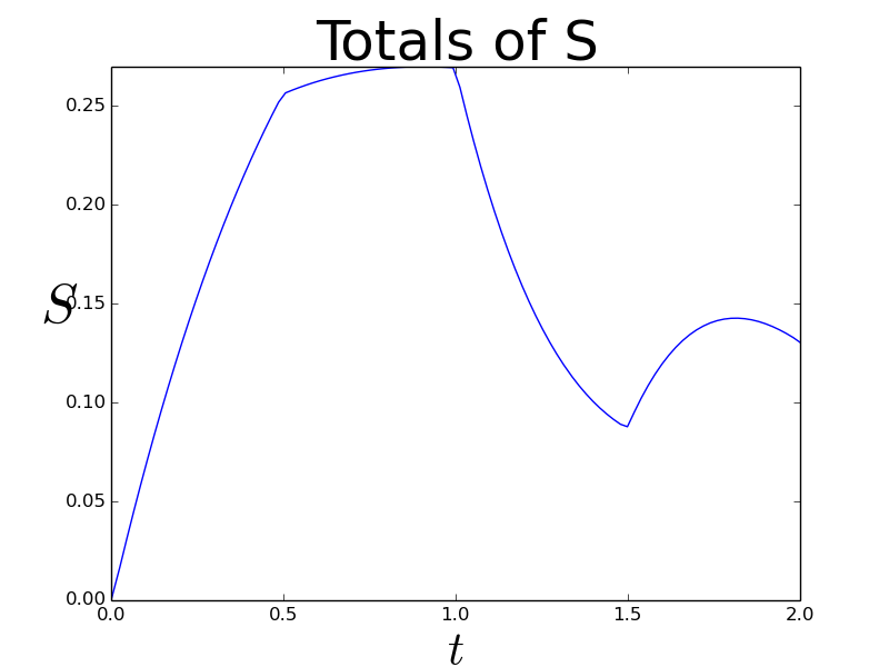 Figure 6
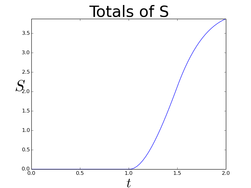 Figure 7
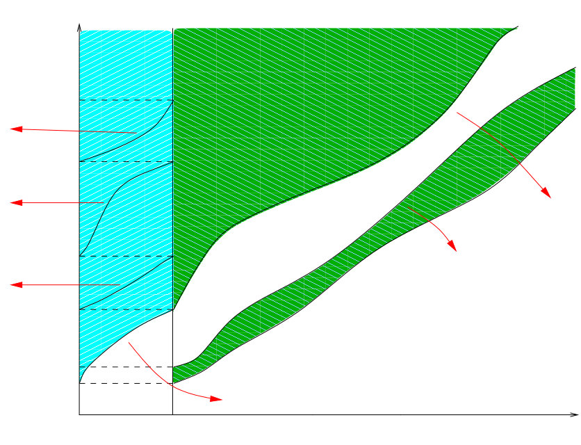 Figure 8
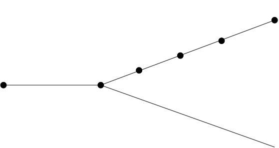 Figure 9
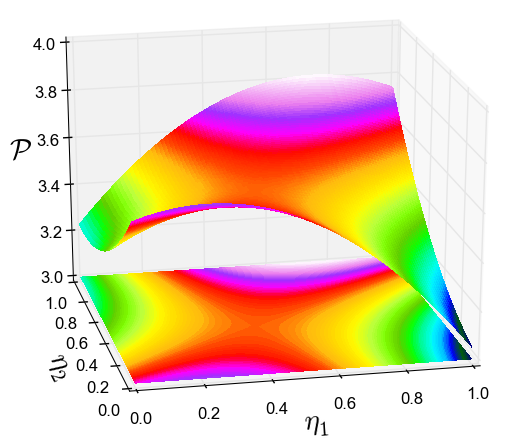 Figure 10
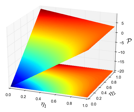 Figure 11
Peer Reviews
No public reviews on file for this paper yet. If you reviewed it on a platform where reviews are public (OpenReview, ICLR, NeurIPS, ICML), you can paste yours below so the community can read it here.
Videos
No videos yet. Explain this paper in a talk, walkthrough, or lecture? Add one.
Taxonomy
TopicsEvolution and Genetic Dynamics · Advanced Thermodynamics and Statistical Mechanics · Mathematical Biology Tumor Growth
11footnotetext: INDAM Unit, University of Brescia22footnotetext: Department of Mathematics and Applications, University of Milano Bicocca
Polynomial Profits in Renewable Resources Management
Rinaldo M. Colombo1
Mauro Garavello2
Abstract
A system of renewal equations on a graph provides a framework to describe the exploitation of a biological resource. In this context, we formulate an optimal control problem, prove the existence of an optimal control and ensure that the target cost function is polynomial in the control. In specific situations, further information about the form of this dependence is obtained. As a consequence, in some cases the optimal control is proved to be necessarily bang–bang, in other cases the computations necessary to find the optimal control are significantly reduced.
Keywords: Management of Biological Resources; Optimal Control of Conservation Laws; Renewal Equations.
2010 MSC: 35L50, 92D25
1 Introduction
A biological resource is grown to provide an economical profit. Up to a fixed age , this population consists of juveniles whose density at time and age satisfies the usual renewal equation [12, Chapter 3]
[TABLE]
and being, respectively, the usual growth and mortality functions, see also [5, 6, 11]. For further structured population models, we refer for instance to [3, 4, 8, 9, 13].
At age , each individual of the population is selected and directed either to the market to be sold or to provide new juveniles through reproduction. Correspondingly, we are thus lead to consider the and the populations whose evolution is described by the renewal equations
[TABLE]
with obvious meaning for the functions . Here, the selection procedure is described by a parameter , varying in , which quantifies the percentage of the population directed to the market, so that
[TABLE]
The overall dynamics is completed by the description of reproduction, which we obtain here through the usual age dependent fertility function using the following nonlocal boundary condition
[TABLE]
In this connection, we recall the related results [1, 2, 7] in structured populations that take into consideration a juvenile–adult dynamics.
Once the biological evolution is defined, we introduce the income and cost functionals as follows. The income is related to the withdrawal of portions of the population at given stages of its development. More precisely, we assume there are fixed ages , with , where the fractions of the population are kept, while the portions are sold. A very natural choice is to set , meaning that nothing is left unsold after age . The dynamics of the whole system has then to be completed introducing the selection
[TABLE]
that takes place at the age , for .
Summarizing, the dynamics of the structured population is thus described by the following nonlocal system of balance laws, see also Figure 1:
[TABLE]
where we inserted the initial data .
Our key result is the proof that for all and all , the quantities , and are polynomial in the values attained by the control parameters and .
We now pass to the introduction of the expressions of cost and income. To this aim, we first fix a time horizon , with . Then, a reasonable expression for the income is
[TABLE]
The latter term above is the sum of the incomes due to the selling of the individuals at the ages . Typically, each value function can be chosen linear in its second argument, but the present framework applies also to the more general polynomial case. The former term in the right hand side of (1.2), namely , accounts for the total amount of the population at time and it can also be seen as the capital consisting of the biological resource at time . Neglecting this term obviously leads to optimal strategies that leave no juveniles at the final time . The value function is also assumed to be polynomial, see Section 3.3.
To model the various costs, we use a general integral functional of the form
[TABLE]
The cost functions , for , are assumed to be polynomial in , for all and . In the simplest case of linear cost and income, (1.2) and (1.3) reduce to
[TABLE]
Here, is the unit value of juveniles of age , while is the price at time per each individual of the population sold at maturity . Similarly, the quantity , for , is the unit cost related to the keeping of individuals of the population , of age , at time .
Below, we provide the essential tools to establish effective numerical procedures able to actually compute the profit
[TABLE]
as a function of the (open loop) control parameters and . In particular, this also allows to find choices of the time dependent control parameters and that allow to maximize . Moreover, the procedures presented below provide an alternative to the use of bang-bang controls. For a comparison between the two techniques we refer to Section 3.3.
The next section presents the main results of this note, while specific examples are deferred to paragraphs 3.1, 3.2 and 3.3. All analytic proofs are in Section 4.
2 Main Results
Throughout we denote , while is the usual characteristic function of the set , so that if and only if , whereas vanishes outside . The positive integers and are fixed throughout, as also the positive strictly increasing real numbers , . It is also of use to introduce the real intervals , , and .
Below, for a real valued function defined on an interval , we call its total variation, while is the set of real valued functions with finite total variation, namely:
[TABLE]
We posit the following assumptions:
(A)
For , the growth rate and mortality rate satisfy
[TABLE]
for a suitable , while the fertility function satisfies .
(ID)
, and .
(P)
and for . Moreover, the map , respectively for , is a polynomial of degree at most in for all , respectively in for .
(C)
and the map is a polynomial of degree at most in , for .
Above, the restriction to of the initial data is not necessary from the analytic point of view, but it is justified by the biological meaning of the variables. Clearly, the extension to the case of polynomials with different degrees is essentially a mere problem of notation.
Recall, as in [6, 11], the strictly increasing sequence of generation times recursively defined for , by
[TABLE]
the characteristic functions and being defined in (4.3) for . If satisfies (A), then the sequence is well defined and as . The interval is the time period when the juveniles of the -th generation are born.
The following results apply to the case of a constant and a constant , when system (1.1) fits into [5, Theorem 2.4] and turns out to be well posed in .
Lemma 2.1** ([5, Corollary 3.4]).**
Let (A) hold. For every , and every initial data as in (ID), system (1.1) admits a unique solution such that
[TABLE]
and the stability estimates in [5, Theorem 2.4 and Theorem 2.5] hold.
In order to exhibit the existence and to actually find a value of and that maximizes as defined in (1.6), we first investigate the regularity of and , defined in (1.2) and (1.3), as functions of the control parameters and .
Lemma 2.2** ([11, Theorem 2.2]).**
Let (A) hold. Let satisfy (C) and the functions and satisfy (P). For every , every , every and every initial data as in (ID),
the maps , , , and are all polynomials in ; 2. 2.
the maps , , are affine in each component of , separately, while the map is polynomial in each component of .
Hence, all the maps , , and are continuously differentiable in both and .
When the control parameters are time dependent, the well posedness of (1.1) follows from [6, Theorem 2.1], which we recall here for completeness.
Theorem 2.3** ([6, Theorem 2.1]).**
Pose conditions (A), (ID). For any and , system (1.1) admits a unique solution. Moreover,
[TABLE]
and there exists a function , with , dependent only on , , , , , and such that for all initial data and and for all controls , , and , the corresponding solutions and to (1.1) satisfy, for every , the following stability estimate:
[TABLE]
Recall the following definition, which allows us to describe the form of the cost, income, and profit as functions of the controls.
Definition 2.4** ([10, Definition 4.1.2]).**
A map is multiaffine if is affine as a function of each , for , (keeping all other fixed).
The elementary property below of multiaffine functions plays a key role in selecting those situations where a bang–bang control may yield the optimal profit. Its proof is deferred to Section 4.
Lemma 2.5**.**
Let and be multiaffine and not constant. Then, admits neither points of strict local minimum, nor points of strict local maximum. Hence, is attained on a vertex of .
The two theorems below constitute the main results of the present work.
Theorem 2.6**.**
Pose conditions (A), (ID). Introduce times such that
[TABLE]
and control parameters for . Let be the solution to (1.1) corresponding to the control
[TABLE]
Then, for all and , the quantities , and are multiaffine in .
Remark that the latter condition in (2.2) can always be met, through a suitable splitting of the intervals .
Theorem 2.7**.**
Pose conditions (A), (ID). Introduce times such that
[TABLE]
and control parameters for and . Let be the solution to (1.1) corresponding to the controls
[TABLE]
Then, for all , if , the quantity is multiaffine in the variables .
Corollary 2.8**.**
Pose conditions (A), with constant in time, (ID), (P) and (C). Choose controls as in (2.2)–(2.3) and as in (2.4). Then, the net profit defined in (1.6) is polynomial in and of degree at most in each of the (scalar) variables separately. Moreover, globally, it is a polynomial of degree at most in and of degree at most in .
Thanks to the form of the costs and of the gains ensured by (P) and (C), the proof is an immediate consequence of Theorem 2.6 and Theorem 2.7.
Remark 2.9**.**
A direct consequence of Corollary 2.8 in the case (1.4)–(1.5) of linear gains and costs, thanks to Lemma 2.5, is that optimal controls , among those of the form (2.4), can be found restricting the search to only bang–bang controls, i.e., to those assuming only the values [math] and . Nevertheless, in [6, Theorem 1.8], it is proved that bang-bang controls well approximate the optimal ones, found in the class of for and of for , provided the cost and income are linear, i.e. in the form (1.4)-(1.5).
3 Examples
The examples in paragraphs 3.1 and 3.2 rely on several numerical integrations of (1.1). They were accomplished using the explicit formula (4.2). To compute the gains and the costs (1.2)–(1.3), we used the standard trapezoidal rule.
For simplicity, we assume throughout that at age all the population is sold; this corresponds to the case .
3.1 A Generational Control
We particularize Theorem 2.3 to the case of as in (2.2)–(2.3) with , so that is constant on each generation. On the other hand, we keep constant.
Corollary 3.1**.**
Pose conditions (A), (ID), (P) and (C). Choose linear gains and costs as in (1.4)–(1.5). Let be as in (2.1). Set
[TABLE]
and let be constant. Then, the net profit defined in (1.6) is multiaffine in . Therefore, the optimal profit can be obtained through a bang–bang control.
In the present case (3.1) there are distinct bang–bang controls: Corollary 3.1 ensures that one of them yields the maximum profit. At the same time, the profit is a multiaffine function in , so that it contains at most terms. Therefore, the integration of suitable instances of (1.1) permits to obtain all the coefficients in the expression of as a function of and, hence, to compute for all (i.e., not necessarily bang–bang) possible controls (3.1).
Consider the situation corresponding to the time interval , we have
[TABLE]
and Corollary 3.1 ensures that the profit defined at (1.4)–(1.5)–(1.6) is actually a multiaffine function of , so that
[TABLE]
In other words, thanks to the qualitative information provided by Corollary 3.1, computing only times allows to obtain the expression of valid for all .
As an example, we consider the setting (1.1)–(1.4)–(1.5) defined by the choices:
[TABLE]
Using the expression (4.2) of the exact solution to (1.1) we obtain (up to the second decimal digit)
[TABLE]
so that
[TABLE]
Coherently with the results above, the maximum of is attained at the bang–bang control , see Figure 2. This strategy amounts to first keep all juveniles for reproduction and then sell them all.
3.2 A Periodic Control
We now consider the case of a growth function independent of time. Then, with reference to (2.1), we have for all . It is then natural to consider a piecewise constant control which is periodic and with period :
[TABLE]
Corollary 3.2**.**
Pose conditions (A), (ID), (P) and (C). Assume that the growth function is independent of time. Choose as in (3.3) with for a given and let be constant. Then, the net profit defined in (1.4)–(1.5)–(1.6) is a polynomial of degree at most in .
The proof is a direct consequence of Theorem 2.6 and is hence omitted. Observe that a polynomial of degree in variables contains at most \nu=\left(\begin{array}[]{@{\,}c@{\,}}n+m\\ n\end{array}\right) terms. Therefore, Corollary 3.2 reduces the problem of maximizing (1.6) along the solutions to (1.1) to:
the computation of solutions to (1.1), 2. 2.
the solution to a linear system of equations in variables, 3. 3.
the maximization of a polynomial.
Consider the following example. In the case in (3.3), choosing the time interval , i.e., , we set
[TABLE]
corresponding to , and . Corollary 3.2 ensures that is a polynomial of degree at most separately in and , so that
[TABLE]
and numerical integrations of (1.1) with the consequent evaluation of (1.6) allow to obtain the coefficients and, hence, the full knowledge of the profit as a function of the control parameters.
We consider now the setting (1.1)–(1.4)–(1.5) defined by the choices:
[TABLE]
Using the expression of the exact solution to (1.1) we obtain (up to the second decimal digit)
[TABLE]
The resulting profit is plotted in Figure 3 as a function of . Remark that the resulting optimal control is not bang–bang. At the times the sharp changes in the graphs of and are due to the sharp changes in the control, as prescribed in (3.4).
3.3 A Stabilizing Strategy
As a further example, we consider the case of a nonlinear profit. A justification for this choice can be the necessity to stabilize the juvenile population to reduce the running costs caused by the population.
Therefore, we consider system (1.1), with an income function of the type (1.2) and a nonlinear cost for the population given by
[TABLE]
Here, the fixed parameter can be seen as the juvenile density that, say, minimizes the running costs. We are thus lead to the maximization of the profit (1.6), with linear income (1.4) and cost (3.7). Let be as in (2.1) and consider a generational control as in (3.1), and piecewise constant controls () as
[TABLE]
where for every and . Then, by the analysis in Section 2, we can assert that the profit (1.6) is a second order polynomial in whose first and zeroth order terms are multiaffine in :
[TABLE]
which is a polynomial defined by
[TABLE]
real coefficients.
Thus, solving times the renewal equations (1.1), computing the corresponding profits (3.9), solving a linear system to get the coefficients allows to obtain an expression for valid for all possible control parameters , . As a comparison, we remark that the total number of bang–bang controls in the present case is and there is no guarantee that the optimal control is of bang–bang type. For a comparison between and , refer to Figure 4.
4 Technical Details
As in [5, 6, 12], we recall that the initial – boundary value problem for the renewal equation
[TABLE]
admits a unique solution that can be explicitly computed integrating along characteristics as
[TABLE]
where the maps and , with and , are defined as
[TABLE]
while the map is given by
[TABLE]
Clearly, the knowledge of the maps , and does not require knowledge of the solution to (4.1) but relies only on the solution to the ordinary differential equation (4.3).
Proof of Lemma 2.5. The proof is by induction on . If , then and the proof follows by basic calculus. Let now . Assume that is a point of strict local maximum or minimum for the multiaffine function . Then, one can write
[TABLE]
for suitable multiaffine functions . Since has a point of strict local maximum or minimum at , by the inductive assumption the map is constant. Since, the map may not attain a strict local maximum or minimum at , the proof is completed.
Proof of Theorem 2.6 and Proof of Theorem 2.7. Fix an arbitrary time . Lengthy but elementary computations based on Figure 5 show that the component of the solution to (1.1) admits the following representation, for and where we used (4.2)–(4.3)–(4.4) for :
[TABLE]
The population is given by
[TABLE]
and, finally, the population for is
[TABLE]
The expression of for directly follows. Note that the right hand side in the explicit expression above depends only on the values attained by at .
Fix now an index . Clearly, , and are all independent of for . Consider the time interval . By (4.5), see also Figure 5, it is clear that is independent of for
[TABLE]
Clearly, , respectively , is independent of whenever , respectively .
On the strip , the quantity is linear in by (4.7). Similarly, on , by (4.6) is linear in . Again by (4.6) and (4.7), , respectively , is independent of for and , respectively and . Finally, the above considerations and (4.5) ensure that is affine in for and . The proof is thus completed for .
On the basis of (4.5)–(4.6)–(4.7), a straightforward iterative procedure allows to complete the proof related to the dependence of on .
The proof concerning the dependence of on directly follows from (1.1).
Proof of Corollary 3.1. Apply Corollary 2.8 with , use the assumption (3.1) and Lemma 2.5 to complete the proof.
Acknowledgment: This work was partially supported by the 2015–INDAM–GNAMPA project Balance Laws in the Modeling of Physical, Biological and Industrial Processes.
The reference list from the paper itself. Each links out to its DOI / PubMed record.
- 1[1] A. S. Ackleh and K. Deng. A nonautonomous juvenile-adult model: well-posedness and long-time behavior via a comparison principle. SIAM J. Appl. Math. , 69(6):1644–1661, 2009.
- 2[2] A. S. Ackleh, K. Deng, and X. Yang. Sensitivity analysis for a structured juvenile–adult model. Comput. Math. Appl. , 64(3):190–200, 2012.
- 3[3] À. Calsina and J. Saldaña. Global dynamics and optimal life history of a structured population model. SIAM J. Appl. Math. , 59(5):1667–1685, 1999.
- 4[4] À. Calsina and J. Saldaña. Basic theory for a class of models of hierarchically structured population dynamics with distributed states in the recruitment. Math. Models Methods Appl. Sci. , 16(10):1695–1722, 2006.
- 5[5] R. M. Colombo and M. Garavello. Stability and optimization in structured population models on graphs. Mathematical Biosciences and Engineering , 12(2):311–335, 2015.
- 6[6] R. M. Colombo and M. Garavello. Control of biological resources on graphs. ESAIM: COCV, to appear , 2016.
- 7[7] J. M. Cushing. A juvenile-adult model with periodic vital rates. J. Math. Biol. , 53(4):520–539, 2006.
- 8[8] O. Diekmann, M. Gyllenberg, J. A. J. Metz, and H. R. Thieme. On the formulation and analysis of general deterministic structured population models. I. Linear theory. J. Math. Biol. , 36(4):349–388, 1998.