Pairs of nodal solutions for a Minkowski-curvature boundary value problem in a ball
Alberto Boscaggin, Maurizio Garrione

TL;DR
This paper proves the existence of multiple pairs of nodal solutions for a Minkowski-curvature boundary value problem in a ball, using a shooting technique and analyzing related one-dimensional problems.
Contribution
It introduces a novel application of shooting methods to establish multiple solutions for a nonlinear Minkowski-curvature PDE in a ball.
Findings
Number of solutions increases with parameter λ
Existence of solutions for radial Neumann problem
Existence of solutions for periodic problem
Abstract
By using a shooting technique, we prove that the quasilinear boundary value problem where is a ball and , has more and more pairs of nodal solutions on growing of the parameter . The radial Neumann problem and the periodic problem for the corresponding one-dimensional equation are considered, as well.
Click any figure to enlarge with its caption.
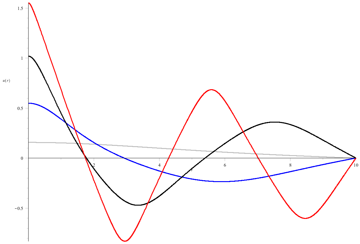 Figure 1
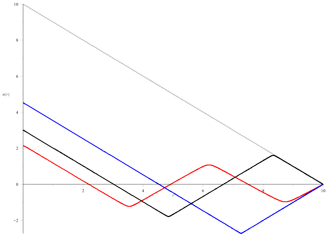 Figure 2
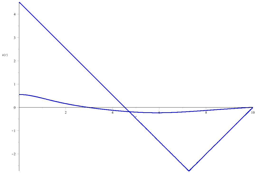 Figure 3
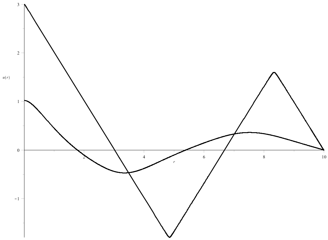 Figure 4
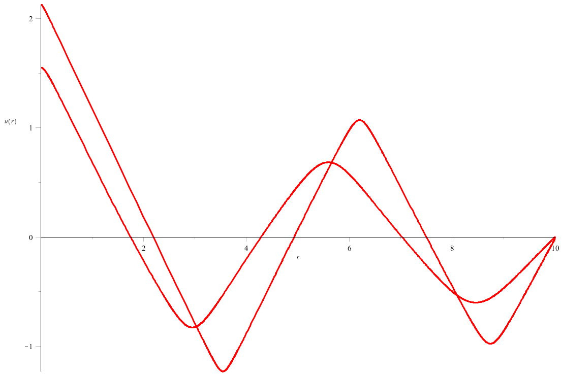 Figure 5
Peer Reviews
No public reviews on file for this paper yet. If you reviewed it on a platform where reviews are public (OpenReview, ICLR, NeurIPS, ICML), you can paste yours below so the community can read it here.
Videos
No videos yet. Explain this paper in a talk, walkthrough, or lecture? Add one.
Taxonomy
TopicsNonlinear Partial Differential Equations · Advanced Mathematical Modeling in Engineering · Differential Equations and Boundary Problems
Pairs of nodal solutions for a Minkowski-curvature boundary value problem in a ball
Alberto Boscaggin
*Dipartimento di Matematica, Università di Torino
via Carlo Alberto 10*, *10123 Torino, Italy
e-mail: [email protected]
*Maurizio Garrione
*Dipartimento di Matematica e Applicazioni, Università di Milano-Bicocca
via Cozzi 55*, *20125 Milano, Italy
e-mail: [email protected]
Abstract
By using a shooting technique, we prove that the quasilinear boundary value problem
[TABLE]
where is a ball and , has more and more pairs of nodal solutions on growing of the parameter . The radial Neumann problem and the periodic problem for the corresponding one-dimensional equation are considered, as well. ††AMS Subject Classification: 35J25, 35J62, 35A24. ††Keywords: radial solutions, Minkowski curvature operator, pairs of solutions, shooting method.
1 Introduction
In this paper, we study existence and multiplicity of radial solutions of the quasilinear equation
[TABLE]
where is the ball of radius , for .
As well known, the above differential equation can be meant as a prescribed mean curvature equation in the Minkowski space [3, 14, 15]; in recent years, the solvability of the associated boundary value problems - even in the non-radial setting - has gained a lot of interest among researchers in the field of Nonlinear Analysis (see, for instance, [4, 5] and the references therein).
The model case for our investigation will be the Dirichlet boundary value problem
[TABLE]
where is a continuous function, and is a positive parameter. As shown in [6, 11], the role of is crucial for the existence of positive solutions of (1.2). In particular, it was proved therein that, when and is large enough, two positive (and two negative) solutions appear, while in general nonexistence holds for (see also [10] for a previous achievement in a one-dimensional setting). Later on, such a result has been extended to the genuine PDE setting in [5, 12].
The aim of this paper is to show that more and more nodal (i.e., sign-changing) solutions of (1.2) appear as well, on growing of the parameter . More precisely, as a corollary of our main result, we can state the following theorem.
Theorem 1.1**.**
Let and let be a continuous function such that for some . Then, for any integer , there exists such that, for every , problem (1.2) has at least nodal radial solutions.
We anticipate that the above solutions will be distinguished according to their number of nodal regions; we refer to Theorem 3.1 for a precise description, in a more general setting.
The underlying idea of the high-multiplicity scheme in Theorem 1.1 can be traced back to a paper by Rabinowitz [18], dealing however with a semilinear second order equation like , with for large. Recently, this pattern has been shown to emerge in several different situations, both for ordinary [8] and partial differential equations [16], always requiring a sublinear behavior for at infinity, i.e., . Theorem 1.1 can thus be seen as a further step in this line of research; it is remarkable, however, that the sublinearity of at infinity is not needed, due to the peculiar properties of the Minkowski-curvature operator.
As for the proof of Theorem 1.1, we adopt a shooting approach for the equivalent ODE formulation
[TABLE]
that is, we consider the associated singular Cauchy problem
[TABLE]
on varying of the initial datum , looking for values such that . A careful study shows that small (i.e., ) and large (i.e., ) solutions do not rotate around the origin in the phase-plane , while intermediate ones rotate more and more on growing of . As a consequence, similarly as in [8], a “double-gap” picture for the winding number is created and multiple pairs of solutions with precise nodal characterization can be provided.
It is worth noticing that the above argument also allows us to easily recover the existence of four one-signed radial solutions (two positive ones and two negative ones) already proved in [6, 11] with topological and variational techniques, respectively, see Remark 4.1. Incidentally, we mention that a shooting approach has been recently exploited to investigate the existence of radial ground-state solutions, as well [1, 2].
The plan of the paper is the following. In Section 2 we present a preliminary technical result, providing solutions rotating around the origin for a general planar Hamiltonian system. In Section 3 we state and prove our main result, dealing with a nonlinearity of the type , under minimal assumptions on . We then show some numerical simulations in order to ease the reader’s comprehension of the statement. Finally, Section 4 is devoted to several remarks about possible extensions and related results. In particular, we deal with the periodic problem for the one-dimensional counterpart of (1.1), namely
[TABLE]
often used to model the relativistic version of Newton’s law (see [17] and its rich bibliography).
2 An auxiliary result
In this section, we are going to present an auxiliary result dealing with a planar Hamiltonian system of the type
[TABLE]
where are locally Lipschitz continuous functions. Roughly speaking, we are going to prove that, whenever suitable (local) sign-conditions are assumed, the number of rotations around the origin of the planar path becomes arbitrarily large on growing of the width of the interval .
To this end, we will write (whenever possible, namely for ) solutions of (2.1) in (clockwise) polar coordinates as
[TABLE]
with . Notice that, of course, the angular coordinate is defined up to integer multiples of ; however, the expression , for any , is uniquely determined, depending on the path only.
With this in mind, we state and prove the following result, which is a slight variant of [8, Lemma 3.2].
Proposition 2.1**.**
Let , with , be locally Lipschitz continuous functions such that
[TABLE]
Then, for every positive integer , there exist and such that, for every interval with and for every locally Lipschitz continuous functions satisfying
[TABLE]
and
[TABLE]
it holds that any solution of (2.1), defined on and satisfying , fulfills for every and
[TABLE]
Sketch of the proof.
We are going to give a sketch of the proof, following the arguments in [8, Lemma 3.2]. The crucial point is to construct two spiraling planar curves controlling (from below and from above) the rotations of the planar path ; this can be done be gluing together pieces of level curves of suitable energy functions. Precisely, after having extended and to the whole real line in such a way that (2.3) still holds and that the primitives
[TABLE]
are coercive, one defines the energies
[TABLE]
Straightforward computations show that, along a solution of (2.1), it holds
[TABLE]
and
[TABLE]
Therefore, the aforementioned parameterized spirals
[TABLE]
can be obtained solving the differential equations
[TABLE]
where
[TABLE]
and
[TABLE]
The remaining part of the proof follows exactly as in [8, Lemma 3.2]. ∎
3 Statement and proof of the main result
In this section, we state and prove our main result concerning the problem
[TABLE]
where is the ball of radius , for , and .
Theorem 3.1**.**
Let be a continuous function such that for some and let be a locally Lipschitz continuous function satisfying
there exists such that
[TABLE]
and
[TABLE]
Then, for any integer , there exists such that, for every , problem (3.1) has at least sign-changing radial solutions. More precisely, for every integer there exist four radial solutions , , , of (3.1) satisfying
[TABLE]
and having exactly nodal domains.
Theorem 1.1 in the Introduction is a direct consequence of this statement for , which satisfies assumption as long as . Notice however that in Theorem 3.1 only a local condition on at zero is required. We also observe that the solutions found are distinguished through their nodal properties; precisely, for any , we find four solutions, two of them with positive value in the center of the ball (a small one and a large one ) and two with negative value therein (a small one and a large one ); see Section 3.2 for a more accurate discussion.
3.1 Proof of Theorem 3.1
Setting
[TABLE]
and writing with the usual abuse of notation, we convert the radial problem associated with (3.1) into
[TABLE]
Remark 3.1**.**
Let us recall that a solution of (3.2) is meant as a function such that for every , and the differential equation in (3.2) is satisfied pointwise, together with the boundary conditions. Actually, by an easy regularity argument (see [11, Remark 3.3]) one can see that , finally implying .**
As a first step, we are going to introduce an equivalent formulation of this problem, obtained from a suitable modification of both the differential operator and the nonlinear term (cf. [11, Proposition 2.1]). Precisely, on one hand we choose a locally Lipschitz continuous function such that
[TABLE]
and we set . On the other hand, we set and define the -function as
[TABLE]
We then introduce the modified problem
[TABLE]
meaning its solutions as in Remark 3.1 (up to the requirement ), and state the following lemma.
Lemma 3.1**.**
Let ; then, is a solution of (3.2) if and only if is a solution of (3.3).
Proof.
Let be a solution of (3.3); integrating the equation and using , we obtain
[TABLE]
implying
[TABLE]
Hence, on one hand for every ; on the other hand, using we have that
[TABLE]
so that , as well. Summing up, solves (3.2).
The converse (which will not be used for our purposes) follows from similar arguments and we omit the proof. ∎
According to Lemma 3.1, from now on we deal with problem (3.3). Having in mind the shooting approach presented in the Introduction, we first state a global existence and continuous dependence result for the associated Cauchy problems.
Lemma 3.2**.**
For any , the Cauchy problem
[TABLE]
has a unique solution defined on . Moreover, if , then
[TABLE]
uniformly on .
Proof.
We first observe that is a solution of (3.6), defined on , if and only if it is a fixed point of the operator defined by
[TABLE]
incidentally, we explicitly notice that is well-defined, despite the presence of the singular term . We are going to establish existence and uniqueness of a fixed point by proving that a suitable iterate of is a contraction with respect to the standard sup-norm . Precisely, denoting by and the Lipschitz constants of and respectively, and setting
[TABLE]
we show by induction that, for every and for every , , it holds
[TABLE]
from which the thesis easily follows for large enough.
For , the estimate (3.8) is trivial. Assuming it for , we have
[TABLE]
thus implying that (3.8) holds true.
The first convergence in (3.7) is a direct consequence of the above argument, while the second one now follows directly by integrating the differential equation in (3.6). ∎
Henceforth, we set
[TABLE]
and we pass to (clockwise) polar-like coordinates, by writing
[TABLE]
where for and for . Notice that this change of variables is admissible for , since
[TABLE]
this being a consequence of the uniqueness of the Cauchy problems (indeed, on the differential equation in (3.3) can be written as a first order planar system satisfying the assumption of Cauchy-Lipschitz theorem). Moreover, by standard results on path liftings, the continuity of the path with respect to ensures that depends continuously on , as well.
We also highlight the following property of the function , which will be used in the proofs.
Lemma 3.3**.**
For every such that , it holds that
[TABLE]
Proof.
The result follows easily from the fact that
[TABLE]
whence if , namely if and (see also [8, Lemma 3.1]). ∎
From now on, we consider the case when and show how to find the solutions for . A symmetric argument yields the other pairs of solutions.
According to the general strategy described in the Introduction, we first focus on the behavior of the small solutions; without loss of generality, we take the constant appearing in assumption strictly less than .
Lemma 3.4**.**
For every , there exists such that, for any , it holds that
[TABLE]
Proof.
Let us fix and choose such that
[TABLE]
By assumption , there exists such that
[TABLE]
By Lemma 3.2, we finally find such that, if , it holds
[TABLE]
With these positions, we are going to prove that the planar path , for , cannot reach the negative -semiaxis, which clearly implies the conclusion.
By contradiction, suppose that this is not the case. Then, there exists such that the path satisfies
[TABLE]
Of course, also the path
[TABLE]
satisfies (3.12); as a consequence, passing to clockwise polar coordinates as in (2.2), we find
[TABLE]
that is, in view of the differential equation in (3.3),
[TABLE]
Recalling that for every and using (3.10)-(3.11), together with the inequality , we finally obtain
[TABLE]
contradicting (3.9). ∎
Second, we prove our key lemma; roughly speaking, we make larger solutions rotate as desired by enlarging the parameter .
Lemma 3.5**.**
For every integer , there exists such that for every there exists such that
[TABLE]
Proof.
We first choose such that for and state the following.
Claim. There exist and such that, for every , every solution of (3.3) satisfying fulfills
[TABLE]
Proof of the claim. We set
[TABLE]
for . It is easily seen that solves the differential system
[TABLE]
In view of the choice of , we have that, for every and , it holds that
[TABLE]
On the other hand, since
[TABLE]
we find that, for every and ,
[TABLE]
Taking into account that, denoting by the angular coordinate associated with the planar path as in (2.2), it holds that
[TABLE]
Proposition 2.1 can be applied with the choice , providing
[TABLE]
∎
We can now easily draw the conclusion: indeed, it holds that and , since for . Accordingly, recalling that , there exists such that
[TABLE]
Since
[TABLE]
from the previous Claim and Lemma 3.3 the statement follows. ∎
We are now in a position to conclude. Given , we fix (where is given by Lemma 3.5) and we consider the continuous function
[TABLE]
Of course, ; moreover, from Lemmas 3.4 and 3.5 we infer that and that
[TABLE]
Then, the Intermediate Value theorem gives, for any integer , two positive values , with
[TABLE]
such that
[TABLE]
The solutions
[TABLE]
are therefore distinct solutions of (3.2); moreover, from (3.14), together with the fact that whenever (compare with the proof of Lemma 3.3), it follows that and have exactly zeros on (see also [8, Lemma 3.8]).
A similar argument works when , giving the other pair of solutions.
3.2 Some numerical simulations
To give a better insight into the statement of Theorem 1.1, we collect here below some numerical simulations obtained with MAPLE*©* software (see Figures 1, 2 and 3 below) for the equation
[TABLE]
choosing and . The Dirichlet solutions shown are found for ; for completeness, we also depict the one-signed solutions already found in [6, 11] (see Remark 4.1).
The reader will certainly notice how the large solutions found above appear almost sharp-cornered, with slope approximately equal to ; we remark that, in principle, this is not a drawback of numerics but rather a consequence of the peculiar properties of the Minkowski curvature operator, as an elementary singular perturbation analysis shows. For simplicity, we assume that for every and for every and we discuss the case when is a family of positive solutions of (3.1). Passing to the radial formulation, it is immediate to see that is decreasing; moreover, using the arguments in the proof of Lemma 3.1, we obtain that is bounded in the -norm. By the sequential version of the Banach-Alaoglu theorem, there exists such that, up to subsequences, in the weak∗-topology of . Notice that is nonnegative and nonincreasing. Of course, it may be that (indeed, this is the case for the family of small positive solutions); however, assume that on , for some . Setting and recalling that , we have
[TABLE]
By Fatou Lemma, for any , so that for any . By Lebesgue theorem, strongly in for every , so that (notice that, a posteriori, ) and strongly in for every . Notice that this convergence is sharp: indeed, since and , if the convergence were it should be (while ). The same argument works for negative solutions and, with some more care, is extendable to nodal solutions as well, showing that the graph of the singular limit is a polygonal line with slopes and .
4 Final remarks
We conclude the paper with some final remarks about possible extensions of Theorem 1.1 and related results.
Remark 4.1**.**
One-signed solutions. The choice in (3.14) is admissible, as well. In this way, the existence of four one-signed (two positive and two negative) radial solutions directly follows (compare with [6, 11]).
Remark 4.2**.**
The Neumann problem. With similar arguments, we can deal as well with the Neumann problem
[TABLE]
Indeed, when passing to the ODE formulation, one is led to the Neumann problem
[TABLE]
and it is possible to find solutions by imposing, instead of (3.14), the condition , for any integer . It has to be noticed, however, that an analogue of Lemma 3.1 can still be established only due to the fact that we deal with nodal solutions (ensuring the validity of (3.5)). Incidentally, we observe that in fact one-signed solutions of the Neumann problem typically do not exist (choose and integrate the equation).
Remark 4.3**.**
Solutions on annuli. The same result as in Theorem 3.1 holds true if the ball is replaced by the annular domain . Here, the radial formulation reads as the Dirichlet problem
[TABLE]
and an analogue of Lemma 3.1 holds true also in this case, since both and vanish at least once in (ensuring the validity of formulas (3.4) and (3.5)). One can thus set, for the truncated equivalent problem, the shooting scheme
[TABLE]
and look for solutions satisfying , for . The previous procedure of proof can still be followed, but unexpectedly some extra work is needed. Summarizing the main steps, it should be proved that:
* for small enough, as can be shown using arguments on the lines of the ones in Lemma 3.4;*
- -
* for large enough, this being a consequence of the so-called elastic property (i.e., uniformly when , see [19, Lemma 2] and notice that the differential equation in (4.1) is not anymore singular) and of the fact that for ;*
- -
* for , this being provable as in Lemma 3.5 using the elastic property once more to prove that (3.13) holds true.*
We refer the reader to [8] for a detailed proof following this scheme, even if in a different setting. Combining with the previous Remark 4.2, one deduces the validity of Theorem 3.1 for the Neumann problem on an annulus, as well.
Remark 4.4**.**
The periodic problem. When is a continuous and -periodic function (), a version of Theorem 3.1 can also be stated for the -periodic problem associated with the differential equation
[TABLE]
In this case, instead of using the above shooting procedure, one has to apply the Poincaré-Birkhoff fixed point theorem. We briefly illustrate here below the steps of the proof, referring again the reader to [8]:
we pass to the truncated problem ; the analogue of Lemma 3.1 holds true since both and vanish at least once in (see the corresponding discussions in Remarks 4.2 and 4.3);
- -
we write the truncated equation as the planar Hamiltonian system
[TABLE]
and we denote by the solution satisfying the initial conditions ;
- -
we pass to polar-like coordinates
[TABLE]
- -
we prove that both when is small enough and when it is large enough. This can be done again similarly as in the corresponding steps of Remark 4.3;
- -
we prove that there exists such that, for every , there exists with if . This can be shown as in Lemma 3.5 (without loss of generality, we can assume so that the argument therein can be made slightly simpler).
The conclusion then follows from the Poincaré-Birkhoff fixed point theorem. We also mention that, combining the arguments in the present paper with the ones in [13, Section 3] it should be possible to prove the existence of pairs of subharmonic solutions (namely, -periodic solutions for ) for the equation
[TABLE]
In this case, the largeness of is replaced by the width of the periodicity interval (this requiring, however, that for every ). For the sake of briefness, we omit the details.
Remark 4.5**.**
Some complementary situations. We finally observe that the superlinearity assumption in , namely , is used only to ensure the validity of Lemma 3.4. Accordingly, a “double gap” for the winding number can be established, thus producing solutions in pairs. If no asymptotic hypothesis at zero is required (keeping, however, the validity of the local sign assumption for ), then solutions are still preserved for , thanks to the gap between intermediate and large solutions. Of course, depending on the growth condition at zero, a more precise picture may be displayed. For instance, combining the arguments of the present paper with the ones in [9], it is possible to find, for every (and assuming ), infinitely many nodal radial solutions of the equation
[TABLE]
having any arbitrary integer number of nodal regions. For completeness, we also mention [7] for the case when is linear at zero, in the context of the one-dimensional periodic problem.
Acknowledgement. The authors were supported by the INDAM-GNAMPA Project 2016 “Problemi differenziali non lineari: esistenza, molteplicità e proprietà qualitative delle soluzioni”. The first author also acknowledges the support of the project ERC Advanced Grant 2013 n. 339958 “Complex Patterns for Strongly Interacting Dynamical Systems - COMPAT”.
The reference list from the paper itself. Each links out to its DOI / PubMed record.
- 1[1] A. Azzollini, Ground state solution for a problem with mean curvature operator in Minkowski space , J. Funct. Anal. 266 (2014), 2086–2095.
- 2[2] A. Azzollini, On a prescribed mean curvature equation in Lorentz-Minkowski space , J. Math. Pures Appl. (9) 106 (2016), 1122–1140.
- 3[3] R. Bartnik and L. Simon, Spacelike hypersurfaces with prescribed boundary values and mean curvature , Comm. Math. Phys. 87 (1982/83), 131–152.
- 4[4] C. Bereanu, P. Jebelean and J. Mawhin, Radial solutions for some nonlinear problems involving mean curvature operators in Euclidean and Minkowski spaces , Proc. Amer. Math. Soc. 137 (2009), 161–169.
- 5[5] C. Bereanu, P. Jebelean and J. Mawhin, The Dirichlet problem with mean curvature operator in Minkowski space - a variational approach. , Adv. Nonlinear Stud. 14 (2014), 315–326.
- 6[6] C. Bereanu, P. Jebelean and P.J. Torres, Multiple positive radial solutions for a Dirichlet problem involving the mean curvature operator in Minkowski space , J. Funct. Anal. 265 (2013), 644-659.
- 7[7] A. Boscaggin and M. Garrione, Sign-changing subharmonic solutions to unforced equations with singular ϕ italic-ϕ \phi -Laplacian , Differential and difference equations with applications, 321–329, Springer Proc. Math. Stat., 47 , Springer, New York, 2013.
- 8[8] A. Boscaggin and F. Zanolin, Pairs of nodal solutions for a class of nonlinear problems with one-sided growth conditions , Adv. Nonlinear Stud. 13 (2013), 13–53.