Mixtures of Generalized Hyperbolic Distributions and Mixtures of Skew-t Distributions for Model-Based Clustering with Incomplete Data
Yuhong Wei, Yang Tang, Paul D. McNicholas

TL;DR
This paper introduces flexible mixture models based on generalized hyperbolic and skew-t distributions for robust clustering of incomplete, heavy-tailed, and asymmetric data, with an EM algorithm for parameter estimation and missing data imputation.
Contribution
It develops an analytically feasible EM algorithm for mixture models with missing data, extending robust clustering methods to handle arbitrary missing patterns.
Findings
The proposed methods outperform mean imputation in clustering accuracy.
Simulation studies demonstrate robustness across various missing data proportions.
Real data application confirms practical effectiveness.
Abstract
Robust clustering from incomplete data is an important topic because, in many practical situations, real data sets are heavy-tailed, asymmetric, and/or have arbitrary patterns of missing observations. Flexible methods and algorithms for model-based clustering are presented via mixture of the generalized hyperbolic distributions and its limiting case, the mixture of multivariate skew-t distributions. An analytically feasible EM algorithm is formulated for parameter estimation and imputation of missing values for mixture models employing missing at random mechanisms. The proposed methodologies are investigated through a simulation study with varying proportions of synthetic missing values and illustrated using a real dataset. Comparisons are made with those obtained from the traditional mixture of generalized hyperbolic distribution counterparts by filling in the missing data using the…
Click any figure to enlarge with its caption.
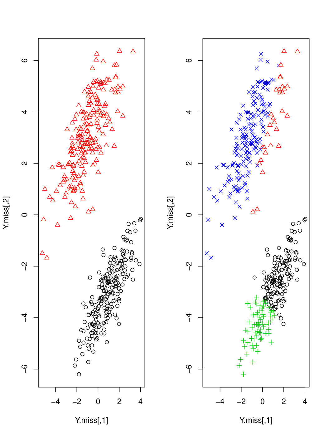 Figure 1
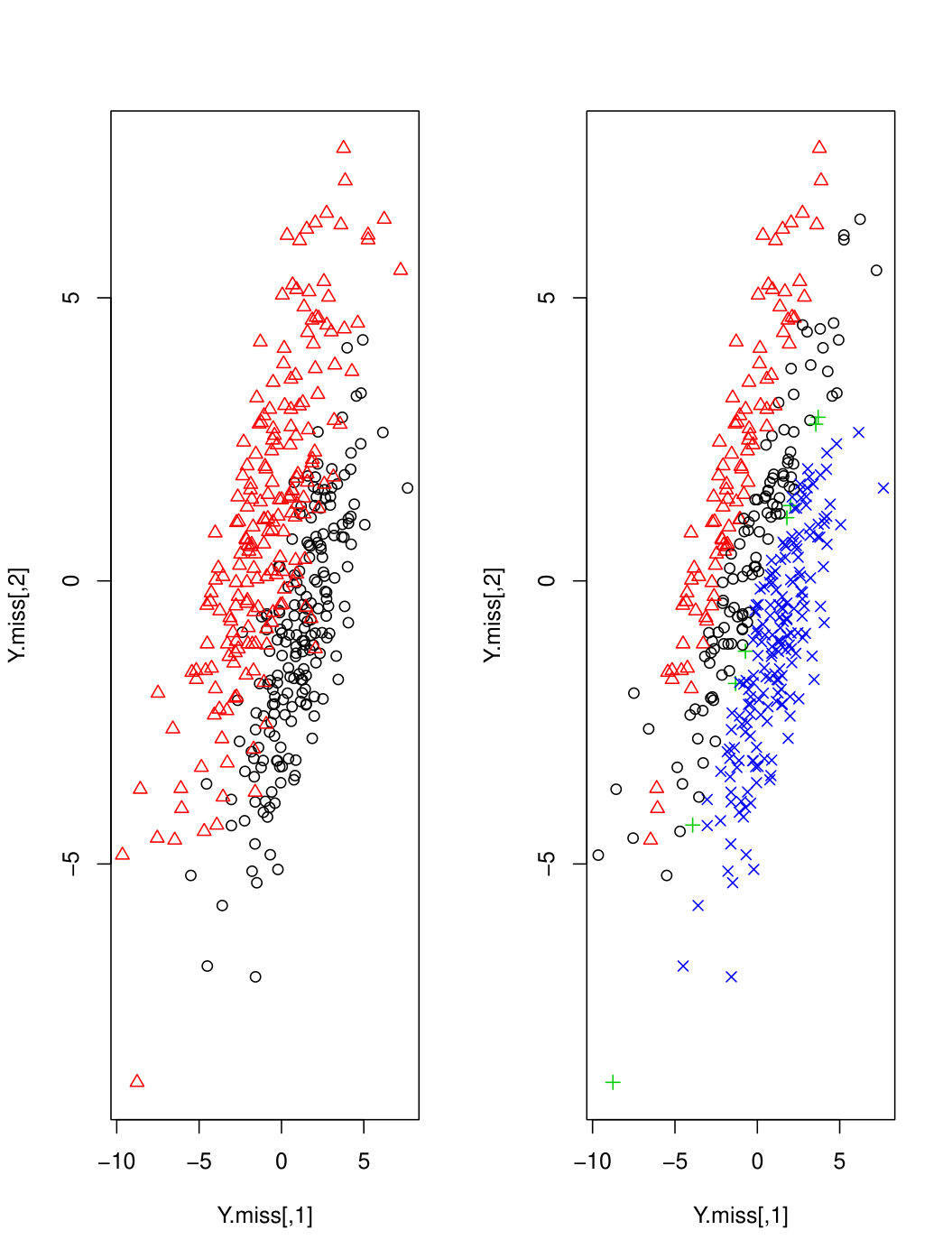 Figure 2
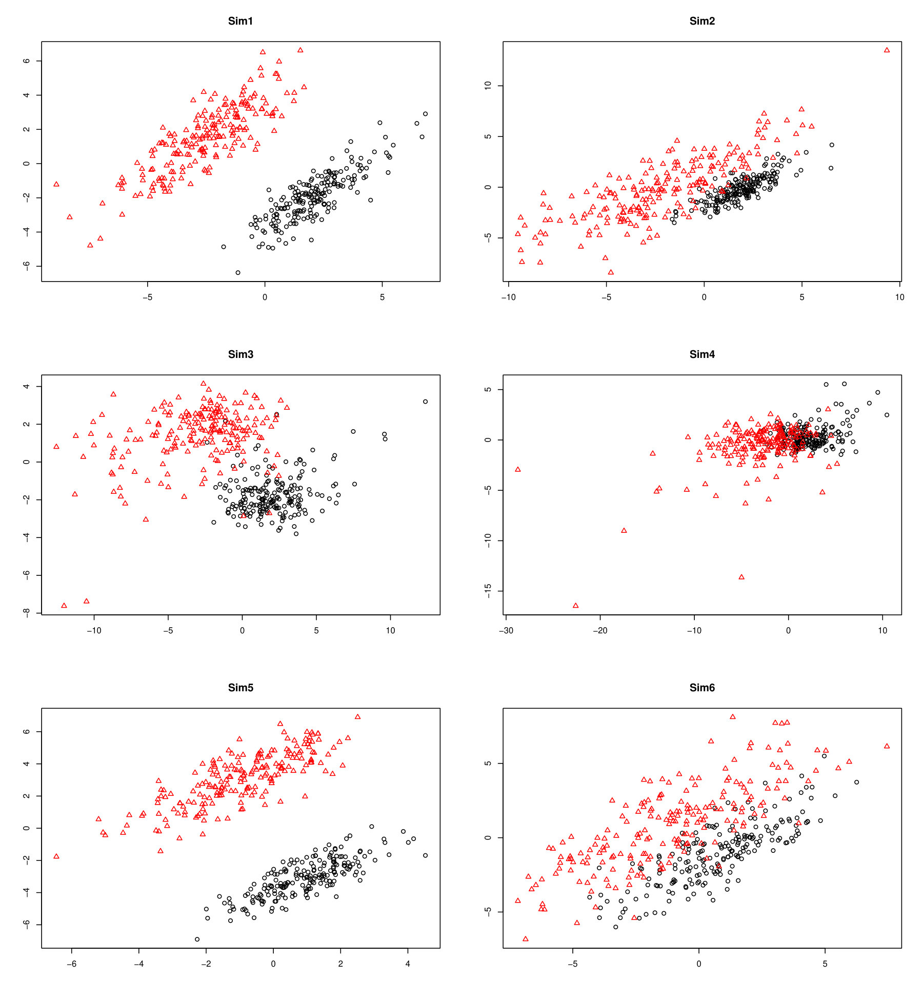 Figure 3
| Dataset | Distribution | Covariance structure | Separation between components |
|---|---|---|---|
| Sim1 | MGHD | VEE | Well-separated |
| Sim2 | MGHD | VEE | Overlapping |
| Sim3 | MST | VEI | Well-separated |
| Sim4 | MST | VEI | Overlapping |
| Sim5 | GMM | VEE | Well-separated |
| Sim6 | GMM | VEE | Overlapping |
| Pattern 1 | Pattern 2 | |
|---|---|---|
| (10,3,6,1) | (1,6,3,10) | |
| (30,9,18,3) | (3,18,9,30) | |
| (60,18,36,6) | (6,36,18,60) |
| Avg.BIC | Avg.ARI | nt | Avg.BIC | Avg.ARI | nt | |
|---|---|---|---|---|---|---|
| MGHD | ||||||
| MST | ||||||
| Mt | ||||||
| No. missing values | Sample mean | Sample std. dev. | |
|---|---|---|---|
| Number of times pregnant | 0 | 3.85 | 3.37 |
| Plasma glucose concentration | 5 | 120.89 | 31.97 |
| Diastolic blood pressure (mm Hg) | 35 | 69.11 | 19.36 |
| Triceps skin fold thickness (mm) | 227 | 20.54 | 15.95 |
| 2-hour serum insulin(mu U/mL) | 374 | 79.80 | 115.24 |
| Body mass index | 11 | 31.99 | 7.88 |
| Diabetes pedigree function | 0 | 0.47 | 0.33 |
| Age (years) | 0 | 33.24 | 11.76 |
| BIC | ICL | Accuracy | ||
|---|---|---|---|---|
| MGHD | EVE | 69.11% | ||
| MST | VVI | 62.37% |
| Parameter | ||
|---|---|---|
| (0.11) | 2.98 (1.78) | |
| (0.22) | 1.35 (4.01) | |
| (0.14) | 1.10 (2.65) | |
| 0.15 (0.08) | (4.59) | |
| (1.73) | 0.18 (0.25) | |
| (0.07) | 0.57 (0.78) | |
| (0.12) | (8.41) | |
| (0.31) | (2.04) | |
| 0.57 (0.05) | (1.79) | |
| 0.77 (0.47) | (0.25) | |
| 0.54 (0.40) | (1.18) | |
| 0.53 (0.31) | 0.58 (0.38) | |
| 0.11 (0.13) | 0.11 (0.32) | |
| 0.57 (0.16) | (0.51) | |
| 0.63 (0.18) | 1.27 (0.46) | |
| 0.87 (0.16) | 2.91 (1.85) | |
| 2.39 (1.81) | 14.18 (6.83) | |
| 0.02 (0.34) | (4.60) | |
| 0.71 (0.09) | 0.29 (0.10) |
| Nomenclature | Volume | Shape | Orientation | |
|---|---|---|---|---|
| EII | Equal | Spherical | ||
| VII | Variable | Spherical | ||
| EEI | Equal | Equal | Axis-Aligned | |
| VEI | Variable | Equal | Axis-Aligned | |
| EVI | Equal | Variable | Axis-Aligned | |
| VVI | Variable | Variable | Axis-Aligned | |
| EEE | Equal | Equal | Equal | |
| VEE | Variable | Equal | Equal | |
| EVE | Equal | Variable | Equal | |
| EEV | Equal | Equal | Variable | |
| VVE | Variable | Variable | Equal | |
| VEV | Variable | Equal | Variable | |
| EVV | Equal | Variable | Variable | |
| VVV | Variable | Variable | Variable |
| Sim1 using MGHD | |||||||||
| Pattern 1 | Pattern 2 | MCAR | |||||||
| Mean | Std. dev | Bias | Mean | Std. dev. | Bias | Mean | Std. dev. | Bias | |
| ARI | |||||||||
| Pattern 1 | Pattern 2 | MCAR | |||||||
| Mean | Std. dev | Bias | Mean | Std. dev. | Bias | Mean | Std. dev. | Bias | |
| ARI | |||||||||
| Pattern 1 | Pattern 2 | MCAR | |||||||
| Mean | Std. dev | Bias | Mean | Std. dev. | Bias | Mean | Std. dev. | Bias | |
| ARI | |||||||||
| Sim3 using MST | |||||||||
| Pattern 1 | Pattern 2 | MCAR | |||||||
| Mean | Std. dev | Bias | Mean | Std. dev. | Bias | Mean | Std. dev. | Bias | |
| ARI | |||||||||
| Pattern 1 | Pattern 2 | MCAR | |||||||
| Mean | Std. dev | Bias | Mean | Std. dev. | Bias | Mean | Std. dev. | Bias | |
| ARI | |||||||||
| Pattern 1 | Pattern 2 | MCAR | |||||||
| Mean | Std. dev | Bias | Mean | Std. dev. | Bias | Mean | Std. dev. | Bias | |
| ARI | |||||||||
| MGHD | MST | Mt | |||||
|---|---|---|---|---|---|---|---|
| BIC | ARI | BIC | ARI | BIC | ARI | ||
| Sim1 | 0.95 | 0.88 | 0.75 | ||||
| 0.87 | 0.82 | 0.69 | |||||
| 0.74 | 0.69 | 0.60 | |||||
| Sim2 | 0.73 | 0.64 | 0.59 | ||||
| 0.62 | 0.52 | 0.48 | |||||
| 0.46 | 0.36 | 0.36 | |||||
| Sim3 | 0.82 | 0.76 | 0.64 | ||||
| 0.76 | 0.66 | 0.63 | |||||
| 0.70 | 0.60 | 0.48 | |||||
| Sim4 | 0.72 | 0.41 | 0.33 | ||||
| 0.60 | 0.37 | 0.27 | |||||
| 0.12 | 0.23 | 0.20 | |||||
| Sim5 | 0.94 | 0.74 | 0.88 | ||||
| 0.85 | 0.66 | 0.78 | |||||
| 0.71 | 0.59 | 0.64 | |||||
| Sim6 | 0.68 | 0.40 | 0.38 | ||||
| 0.58 | 0.38 | 0.35 | |||||
| 0.40 | 0.28 | 0.29 | |||||
Peer Reviews
No public reviews on file for this paper yet. If you reviewed it on a platform where reviews are public (OpenReview, ICLR, NeurIPS, ICML), you can paste yours below so the community can read it here.
Videos
No videos yet. Explain this paper in a talk, walkthrough, or lecture? Add one.
Mixtures of Generalized Hyperbolic Distributions and Mixtures of Skew-t Distributions for Model-Based Clustering with Incomplete Data
Yuhong Wei, Yang Tang and Paul D. McNicholas
(Dept. of Mathematics & Statistics, McMaster University, Hamilton, Ontario, Canada.)
Abstract
Robust clustering from incomplete data is an important topic because, in many practical situations, real data sets are heavy-tailed, asymmetric, and/or have arbitrary patterns of missing observations. Flexible methods and algorithms for model-based clustering are presented via mixture of the generalized hyperbolic distributions and its limiting case, the mixture of multivariate skew-t distributions. An analytically feasible EM algorithm is formulated for parameter estimation and imputation of missing values for mixture models employing missing at random mechanisms. The proposed methodologies are investigated through a simulation study with varying proportions of synthetic missing values and illustrated using a real dataset. Comparisons are made with those obtained from the traditional mixture of generalized hyperbolic distribution counterparts by filling in the missing data using the mean imputation method.
Keywords: Clustering; generalized hyperbolic; missing data; mixture models; skew-t.
1 Introduction
Finite mixture models are powerful and flexible tools for discovering unobserved heterogeneity in multivariate datasets. Assuming no prior knowledge of class labels, the application of finite mixture models in this way is known as model-based clustering. As McNicholas (2016a) points out, the association between mixture models and clustering goes back at least as far as Tiedeman (1955), who uses the former as a means of defining the latter. Gaussian mixture models are historically the most popular tool for model-based clustering and dominated the literature for quite some time (e.g., Celeux and Govaert, 1995; Fraley and Raftery, 1998; McLachlan et al., 2003; Bouveyron et al., 2007; McNicholas and Murphy, 2008, 2010). The multivariate -distribution, being a heavy-tailed alternative to the multivariate Gaussian distribution, made (robust) mixture modelling based on mixtures of multivariate -distributions the most natural extension (e.g., Peel and McLachlan, 2000; Andrews and McNicholas, 2011, 2012; Steane et al., 2012; Lin et al., 2014). In many practical situations, however, real world datasets exhibit clusters that are not just heavy tailed but also asymmetric; furthermore, clusters can also be asymmetric yet not heavy tailed. Over the few past years, much attention has been paid to non-Gaussian approaches to model-based clustering and classification, including work on multivariate skew- distributions (e.g., Lin, 2010; Vrbik and McNicholas, 2012; Lee and McLachlan, 2014; Murray et al., 2014a, b, 2017b), shifted asymmetric Laplace distributions (Franczak et al., 2014), multivariate power exponential distributions (Dang et al., 2015), multivariate normal inverse Gaussian distributions (Karlis and Santourian, 2009; O’Hagan et al., 2016), generalized hyperbolic distributions (Browne and McNicholas, 2015; Morris and McNicholas, 2016; Tortora et al., 2016), and hidden truncation hyperbolic distributions (Murray et al., 2017a). A comprehensive review of model-based clustering work, up to and including some recent work on non-Gaussian mixtures, is given by McNicholas (2016b).
Unobserved or missing observations are frequently a hindrance in multivariate datasets and so developing mixture models that can accommodate incomplete data is an important issue in model-based clustering. The maximum likelihood and Bayesian approaches are two common imputation paradigms for analyzing data with incomplete observations. Herein, the missing data mechanism is assumed to be missing at random (MAR), as per Rubin (1976) and Little and Rubin (1987), meaning that the probability that a variable is missing for a particular individual depends only on the observed data and not on the value of the missing variable. Note that missing completely at random (MCAR) is a special case of MAR. Under MAR, the missing data mechanisms are ignorable for methods using the maximum likelihood approach.
The maximum likelihood approach to clustering incomplete data has been well studied and is often used, particularly for Gaussian mixture models (e.g., Ghahramani and Jordan, 1994; Lin et al., 2006; Browne et al., 2013). Wang et al. (2004) present a framework maximum likelihood estimation using an expectation-maximization (EM) algorithm (Dempster et al., 1977) to fit a mixture of multivariate -distributions with arbitrary missing data patterns, which was generalized by Lin et al. (2009) to efficient supervised learning via the parameter expanded (PX-EM) algorithm (Liu et al., 1998) through two auxiliary indicator matrices. Lin (2014) further develops a family of multivariate- mixture models with 14 eigen-decomposed scale matrices in the presence of missing data through a computationally flexible EM algorithm by incorporating two auxiliary indicator matrices. Wang and Lin (2015) uses a formulation of the mixture of skew-t distributions for model-based clustering with missing data.
We consider fitting mixtures of generalized hyperbolic distributions (MGHD) and mixtures of multivariate skew-t distributions (MST) with missing information. In each case, an EM algorithm is used for model selection. The chosen formulation of the (multivariate) generalized hyperbolic distribution (GHD) is that used by Browne and McNicholas (2015) and has formulations of several well-known distributions as special cases such as the multivariate skew-, normal inverse Gaussian, variance-gamma, Laplace, and Gaussian distributions (cf. McNeil et al., 2005). In addition to considering missing data, we develop families of MGHD and MST mixture models, each with 14 parsimonious eigen-decomposed scale matrices corresponding to the famous Gaussian parsimonious clustering models of (GPCMs; Banfield and Raftery, 1993; Celeux and Govaert, 1995); see Table 7 (Appendix A).
2 Background
2.1 Generalized Inverse Gaussian Distribution
A random variable is said to have a generalized inverse Gaussian (GIG) distribution, introduced by (Good, 1953), with parameters , , and if its probability density function is given by
[TABLE]
where , and is the modified Bessel function of the third kind with index . Herein, we write to indicate that a random variable has the GIG density as parameterized in (1). The GIG distribution has some attractive properties (Barndorff-Nielsen and Halgreen, 1977; Blæsild, 1978; Halgreen, 1979; Jørgensen, 1982), including the tractability of the expectations:
[TABLE]
for , and
[TABLE]
Specifically, for and , we have
[TABLE]
Browne and McNicholas (2015) introduce another parameterization of the GIG distribution by setting and . Write ; its density is given by
[TABLE]
for , where is a scale parameter and is a concentration parameter. These two parameterizations of the GIG distribution are important ingredients for building the generalized hyperbolic distribution presented later.
2.2 Generalized Hyperbolic Distribution
Several alternative parameterizations of the GHD have appeared in the literature, e.g., Barndorff-Nielsen and Blæsild (1981), McNeil et al. (2005), and Browne and McNicholas (2015). Barndorff-Nielsen (1977) introduces the generalized hyperbolic distribution (GHD) to model the distribution of the sand grain sizes and subsequent reports described its statistical properties (e.g., Barndorff-Nielsen, 1978; Barndorff-Nielsen and Blæsild, 1981). However, under this standard parameterization, the parameters of the mixing distribution are not invariant by affine transformations. An important innovation was made by McNeil et al. (2005), who gave a new parameterization of the GHD. Under this new parameterization, the linear transformation of GHD remains in the same sub-family characterized by the parameters of the mixing distribution. However, there is an identifiability issue arising under this parameterization. To solve this problem, Browne and McNicholas (2015) give an alternative parameterization.
Following McNeil et al. (2005), a random vector is said to follow a generalized hyperbolic distribution with index parameter , concentration parameters and , location vector , dispersion matrix , and skewness vector , denoted by \mathbf{X}\sim\text{GH}_{p}(\lambda,\chi,\psi,\mbox{\boldmath\mu},\mbox{\boldmath\Sigma},\mbox{\boldmath\alpha}), if it can be represented by
[TABLE]
where , , \mathbf{U}\sim\mathcal{N}(\mathbf{0},\mbox{\boldmath\Sigma}), and the symbol indicates independence. It follows that \mathbf{X}\mid w\sim\mathcal{N}(\mbox{\boldmath\mu}+w\mbox{\boldmath\alpha},w\mbox{\boldmath\Sigma}). So, the density of the generalized hyperbolic random vector is given by
[TABLE]
where \delta(\mathbf{x},\mbox{\boldmath\mu}\mid\mbox{\boldmath\Sigma})=(\mathbf{x}-\mbox{\boldmath\mu})^{\intercal}\mbox{\boldmath\Sigma}^{\raisebox{0.60275pt}{\scriptscriptstyle-1}}(\mathbf{x}-\mbox{\boldmath\mu}) is the squared Mahalanobis distance between and , is the modified Bessel function of the third kind with index , and \mbox{\boldmath\vartheta}=(\lambda,\chi,\psi,\mbox{\boldmath\mu},\mbox{\boldmath\Sigma},\mbox{\boldmath\alpha}) denotes the model parameters. The mean and covariance matrix of are
[TABLE]
respectively, where and are the mean and variance of the random variable , respectively.
Note that, in this parameterization, we need to hold |\mbox{\boldmath\Sigma}|=1 to ensure identifiability. Using |\mbox{\boldmath\Sigma}|=1 solves the identifiability problem but would be prohibitively restrictive for model-based clustering and classification applications. Hence, Browne and McNicholas (2015) develop a new parameterization of the GHD with index parameter , concentration parameter , location vector , dispersion matrix , and skewness vector \mbox{\boldmath\beta}=\eta\mbox{\boldmath\alpha}, denoted by \mathbf{X}\sim\text{GHD}_{p}(\lambda,\omega,\mbox{\boldmath\mu},\mbox{\boldmath\Sigma},\mbox{\boldmath\beta}). Note that . This formulation is given by
[TABLE]
where , , with , and \mathbf{U}\sim\mathcal{N}(\mathbf{0},\mbox{\boldmath\Sigma}). Under this parameterization, the density of the generalized hyperbolic random vector is
[TABLE]
where \delta(\mathbf{x},\mbox{\boldmath\mu}\mid\mbox{\boldmath\Sigma}) and are as described earlier. We use this parameterization when we describe parameter estimation (cf. Section 3).
The following result shows an appealing closure property of the generalized hyperbolic distribution under affine transformation and conditioning as well as the formation of marginal distributions, which is useful for developing new methods presented later. Suppose that is a -dimensional random vector having a generalized hyperbolic distribution as in (9), i.e., \mathbf{X}\sim\text{GHD}_{p}(\lambda,\omega,\mbox{\boldmath\mu},\mbox{\boldmath\Sigma},\mbox{\boldmath\beta}). Assume that is partitioned as , where takes values in and in , with
[TABLE]
where , , and have similar partitions. Furthermore, \mbox{\boldmath\Sigma}_{11} is and \mbox{\boldmath\Sigma}_{22} is .
Proposition 1**.**
Affine transformation of the generalized hyperbolic distribution. If \mathbf{X}\sim\text{GHD}_{p}(\lambda,\omega,\mbox{\boldmath\mu},\mbox{\boldmath\Sigma},\mbox{\boldmath\beta}) and where and , then
[TABLE]
Proof.
The result follows by substituting (8) into . ∎
Proposition 2**.**
The marginal distribution of is a generalized hyperbolic distribution as in (9) with index parameter , concentration parameter , location vector \mbox{\boldmath\mu}_{1}, dispersion matrix \mbox{\boldmath\Sigma}_{11}, and skewness vector \mbox{\boldmath\beta}_{1}, i.e., \mathbf{X}_{1}\sim\text{GHD}_{d_{1}}(\lambda,\omega,\mbox{\boldmath\mu}_{1},\mbox{\boldmath\Sigma}_{11},\mbox{\boldmath\beta}_{1}).
Proof.
The result follows by applying Proposition 1 and choosing ] and . The parameters inherited from the mixing distribution remain the same under the affine transformation and marginal distribution. ∎
Proposition 3**.**
The conditional distribution of given is a generalized hyperbolic distribution as in (6), i.e., \mathbf{X}_{2}\mid\mathbf{X}_{1}=\mathbf{x}_{1}\sim\text{GH}_{d_{2}}(\lambda_{2\mid 1},\chi_{2\mid 1},\psi_{2\mid 1},\mbox{\boldmath\mu}_{2\mid 1},\mbox{\boldmath\Sigma}_{2\mid 1},\mbox{\boldmath\beta}_{2\mid 1}), where
[TABLE]
The proof of Proposition 3 is given in Appendix B.
2.3 The Multivariate Skew- Distribution
There are several alternative formulations of multivariate skew-t distributions appearing in the literature (e.g., Branco and Dey, 2001; Sahu, Dey, and Branco, 2003; Murray, Browne, and McNicholas, 2014a; Lee and McLachlan, 2014). Lin and Lin (2011) develop a mixture of multivariate skew-t distributions incomplete data using the formulation of Sahu et al. (2003). Herein, the formulation of the multivariate skew- distribution arising from the generalized hyperbolic distribution is used. This formulation of the multivariate skew- distribution has been used by Murray et al. (2014a) to develop a mixture of skew- factor analyzers model.
Following McNeil et al. (2005), a x random vector is said to follow a multivariate skew-t distribution with degree of freedom parameter , location vector , dispersion matrix , and skewness vector , denoted by \mathbf{X}\sim\text{ST}_{p}(v,\mbox{\boldmath\mu},\mbox{\boldmath\Sigma},\mbox{\boldmath\beta}), if it can be represented by
[TABLE]
where , , \mathbf{U}\sim\mathcal{N}(\mathbf{0},\mbox{\boldmath\Sigma}), with denoting the inverse Gamma distribution. It follows that \mathbf{X}\mid w\sim\mathcal{N}(\mbox{\boldmath\mu}+w\mbox{\boldmath\beta},w\mbox{\boldmath\Sigma}) and the pdf of the multivariate skew-t random vector is given by
[TABLE]
This formulation of the multivariate skew-t distribution can be obtained as a special case of the generalized hyperbolic distribution by setting and , and letting . Similarly, this formulation of the multivariate skew-t distribution has a closed form under affine transformation and conditioning, and the formation of marginal distributions, which is useful for developing new methods presented later. Suppose that is a -dimensional random vector having the multivariate skew-t distribution as in (12), i.e., \mathbf{X}\sim\text{ST}_{p}(v,\mbox{\boldmath\mu},\mbox{\boldmath\Sigma},\mbox{\boldmath\beta}). Assume that is partitioned as , where takes values in and in , with
[TABLE]
where , , and have similar partitions. Furthermore, \mbox{\boldmath\Sigma}_{11} is and \mbox{\boldmath\Sigma}_{22} is .
Proposition 4**.**
Affine transformation of the multivariate skew-t distribution. If \mathbf{X}\sim\text{ST}_{p}(v,\mbox{\boldmath\mu},\mbox{\boldmath\Sigma},\mbox{\boldmath\beta}) and , where and , then
[TABLE]
Proof.
The proof follows easily by substituting (11) into . ∎
Proposition 5**.**
The marginal distribution of is a multivariate skew-t distribution as in (12) with degree of freedom parameter , location vector \mbox{\boldmath\mu}_{1}, dispersion matrix \mbox{\boldmath\Sigma}_{11}, and skewness vector \mbox{\boldmath\beta}_{1}, i.e., \mathbf{X}_{1}\sim\text{ST}_{d_{1}}(v,\mbox{\boldmath\mu}_{1},\mbox{\boldmath\Sigma}_{11},\mbox{\boldmath\beta}_{1}).
Proof.
The proof follows easily by applying Proposition 4 and choosing ] and . The degree of freedom parameter inherited from the mixing distribution remains invariant under affine transformation and marginal distribution. ∎
Proposition 6**.**
The conditional distribution of given is a generalized hyperbolic distribution as in (6), i.e., \mathbf{X}_{2}\mid\mathbf{x}_{1}\sim\text{GH}_{d_{2}}(\lambda_{2\mid 1},\chi_{2\mid 1},\psi_{2\mid 1},\mbox{\boldmath\mu}_{2\mid 1},\mbox{\boldmath\Sigma}_{2\mid 1},\mbox{\boldmath\beta}_{2\mid 1}), where
[TABLE]
The proof of Proposition 6 is similar to that for Proposition 3, hence is omitted. Similar results for Proposition 4, 5, and 6 have been obtained in Arellano-Valle and Genton (2010).
3 MGHD with Incomplete Data
Let be -dimensional random variables arising from a heterogeneous population with disjoint MGHD subpopulations. That is, each has the density
[TABLE]
where , such that , are the mixing proportions, denotes the model parameters, and f_{\text{GHD}}(\mathbf{X}_{i}\mid\lambda_{g},\omega_{g},\mbox{\boldmath\mu}_{g},\mbox{\boldmath\Sigma}_{g},\mbox{\boldmath\beta}_{g}) is the GHD density defined in (9).
To apply the MGHD model (14) in the clustering paradigm, introduce , where if observation is in component and otherwise. The corresponding random variable , i.e., follows a multinomial distribution with one trial and cell probabilities .
A three-level hierarchical representation of the MGHD model (14) can be expressed by
[TABLE]
The complete-data consist of the observed together with the missing group membership and the latent , for and , and the complete-data log-likelihood is given by
[TABLE]
Browne and McNicholas (2015) present an EM algorithm for parameter estimation with the MGHD when there is no missing data in . We are interested in parameter estimation for the MGHD model (14) when are partially observed with arbitrary missing patterns. The missing data mechanism is assumed to be MAR. Assume now that we split into two components, and that denote the observed and missing components of , respectively. In general, each data vector may have a different pattern of missing features, i.e., , but can be simplified for the sake of clarity.
For each , partition the vector mean \mbox{\boldmath\mu}_{g}=(\mbox{\boldmath\mu}_{g,i}^{\text{o}\intercal},\mbox{\boldmath\mu}_{g,i}^{\text{m}\intercal})^{\intercal}, where \mbox{\boldmath\mu}_{g,i}^{\text{o}} and \mbox{\boldmath\mu}_{g,i}^{\text{m}} denote the sub-vectors of \mbox{\boldmath\mu}_{g} matching the observed and missing components of , respectively. Similarly, the skewness vector is \mbox{\boldmath\beta}_{g}=(\mbox{\boldmath\beta}_{g,i}^{\text{o}\intercal},\mbox{\boldmath\beta}_{g,i}^{\text{m}\intercal})^{\intercal} and the covariance matrix \mbox{\boldmath\Sigma}_{g} as
[TABLE]
correspond to . As a result, in addition to the observed , the missing group membership , and the latent variable , the complete-data also include the missing data . In the framework of the EM algorithm, the missing data are considered to be random variables that are updated in each iteration. Hence, the complete-data log-likelihood (16) is rewritten as
[TABLE]
Given (15), we establish the following:
- •
The marginal distribution of given is
[TABLE]
where is the dimension corresponding to the observed component , which should be exactly written as but here is simplified.
- •
The conditional distribution of given and , according to Proposition 3, is
[TABLE]
where
[TABLE]
- •
The conditional distribution of given , and is
[TABLE]
- •
The conditional distribution of given and is
[TABLE]
After a little algebra, we get the complete data log-likelihood function is
[TABLE]
On the th iteration of the E-step, the expected value of the complete data log-likelihood is computed given the observed data and the current parameter updates \mbox{\boldmath\Theta}^{(k)}. That is, we need to compute \operatorname{\mathbb{E}}(Z_{ig}\mid\mathbf{x}_{i}^{\text{o}};\mbox{\boldmath\Theta}^{(k)}), \operatorname{\mathbb{E}}(W_{ig}\mid\mathbf{x}_{i}^{\text{o}},z_{ig}=1;\mbox{\boldmath\Theta}^{(k)}), \operatorname{\mathbb{E}}(\log W_{ig}\mid\mathbf{x}_{i}^{\text{o}},z_{ig}=1;\mbox{\boldmath\Theta}^{(k)}), \operatorname{\mathbb{E}}({1}/{W_{ig}}\mid\mathbf{x}_{i}^{\text{o}},z_{ig}=1;\mbox{\boldmath\Theta}^{(k)}), \operatorname{\mathbb{E}}(\mathbf{X}_{i}^{\text{m}}\mid\mathbf{x}_{i}^{\text{o}},z_{ig}=1,w_{i};\mbox{\boldmath\Theta}^{(k)}), and \operatorname{\mathbb{E}}(\mathbf{X}_{i}^{\text{m}}(\mathbf{X}_{i}^{\text{m}})^{\intercal}\mid\mathbf{x}_{i}^{\text{o}},z_{ig}=1,w_{i};\mbox{\boldmath\Theta}^{(k)}).
First, let denote the a posteriori probability that -th observation belongs to the -th component of the mixture, based on the observed data:
[TABLE]
Given (2), (3), and (20), we have the following expectations as to the latent variable :
[TABLE]
[TABLE]
For convenience, we use the following notation analogous to Browne and McNicholas (2015): , , , and . For the actual missing data , we will also need the following expectations:
[TABLE]
On the -th iteration of the M-step, the expected value of the complete data log-likelihood is maximized to get the updates for the parameter estimates as follows:
[TABLE]
where
[TABLE]
and
[TABLE]
Finally, the estimates of and are given as solutions to maximize the function
[TABLE]
and the associated updates are
[TABLE]
The family of MGHD mixture models, with 14 parsimonious eigen-decomposed scaled covariance matrices corresponding to the famous GPCM family of models is proposed (see Appendix A for a brief discussion, including nomenclature). Details on the MST with incomplete data are analogous to the MGHD with incomplete data and are provided in Appendix D.
4 Notes on Implementation
4.1 Initial values
It is well known that the EM algorithm can be heavily dependent on the initial values; indeed, good initial values of parameter estimates may speed up convergence. In this study, the following procedure for automatically generating initial values is used, unless otherwise specified.
- •
Fill in the missing values based on the mean imputation method.
- •
Perform -means clustering and use the resulting clustering membership to initialize the a posteriori probability . Accordingly, the initial values for the model parameters are then given by:
[TABLE]
- •
Set the skewness parameter \mbox{\boldmath\beta}_{g}^{(0)} to be close to zero for symmetric data.
- •
When applicable, we set and for the index and concentration parameters, which represents a special case of GHD (i.e., normal-inverse Gaussian) distribution, or set for the near-normality assumption.
To enhance the computational efficiency of the EM algorithm, we update the parameters per missing pattern instead of per individual. We suggest rearranging according to unique patterns of the missing data. The procedure can be implemented as follows:
- •
Build a binary by indicator matrix , with each entry if is missing and otherwise;
- •
Find all unique missing patterns; and
- •
Update parameters per missing pattern instead of per individual.
4.2 Model Selection and Stopping Criterion
In general, the number of mixture components is not known a priori, and needs to be estimated from the data. Two widely used model selection techniques are the Bayesian information criterion (BIC; Schwarz, 1978) and the integrated completed likelihood (ICL; Biernacki et al., 2000), which are given respectively by
[TABLE]
where l(\hat{\mbox{\boldmath\Theta}}) is the maximized log-likelihood evaluated at the maximum likelihood estimate \hat{\mbox{\boldmath\Theta}}, is the number of free parameters, is the number of observations, represents the estimated a posteriori probability that arises from the th component, and MAP denotes the maximum a posteriori probability such that if occurs in the th component and otherwise. The bigger the BIC or ICL value, the better the fitted model.
The EM algorithm can be stopped iterations after the maximum number of iterations, or when the Aitken stopping criterion (Aitken, 1926) is satisfied. The Aitken acceleration at iteration is
[TABLE]
where is the log-likelihood at iterations . This yields an asymptotic estimate of the log-likelihood at iteration :
[TABLE]
(Böhning et al., 1994; Lindsay, 1995), and the EM algorithm is stopped when , provided this difference is positive (McNicholas et al., 2010).
5 Numerical Examples
Studies based on both simulated and real datasets are used to compare the clustering performance of the proposed approach. Our proposed family of models for incomplete data is compared to multivariate t mixture with ML estimation in the presence of missing values (Mt). BIC is used to select the model; models with higher values of BIC are preferable. The adjusted Rand index (ARI; Hubert and Arabie, 1985) is used to compare predicted classifications to true classes when applicable. The Rand index (Rand, 1971) is the ratio of pairwise agreements to total pairs, and the ARI corrects the Rand index to account for chance agreement. The ARI has expected value 0 under random classification and takes the value 1 for perfect class agreement. A detailed discussion of the ARI, and arguments in favour of its use, are given by Steinley (2004).
5.1 Simulation Studies
The simulated datasets are each two-component mixtures: a mixture of Gaussian distributions (GMM) with a general VEE covariance structure, a mixture of skew-t distributions (MST) with a diagonal VEI covariance structure, and a mixture of generalized hyperbolic distributions (MGHD) with a general VEE covariance structure. The GMM datasets are generated via the R function rmvnorm from the mvtnorm package for R, and the MST and MGHD datasets are generated using R code based on the stochastic representations in (11) and (8), respectively.
For each mixture component, two-dimensional vectors are generated. The presumed parameters of \mbox{\boldmath\Sigma}_{g} () for the VEE and VEI models are the same as those considered in Celeux and Govaert (1995) and Lin (2014). Each mixture component is centred on a different point giving well-separated and overlapping mixtures. Where applicable, the skewness parameters are \mbox{\boldmath\beta}_{1}=(1,1)^{\intercal} and \mbox{\boldmath\beta}_{2}=(-1,-1)^{\intercal}, the degrees of freedoms for the MST is and , and the values of other parameters for the MGHD are and and .
The datasets considered in the simulation studies are summarized in Table 1 and examples are plotted in Figure 1. The datasets are overlapping, making this a relatively difficult clustering scenario even when the datasets are complete.
Artificial missing datasets are simulated by removing elements from each column of the simulated samples through two different MAR patterns and the MCAR mechanism under three missing rates — (low), (moderate), and (high) — while maintaining the condition that each observation has at least one observed attribute. For the MAR mechanism, data points in the first column are sorted in descending order. Column is then divided into four equal blocks and, for each block, a specified number of elements (see Table 2) are removed at random. When , the second column is used.
First, we examine the ability of our proposed model to recover underlying parameters when the number of components and the covariance structure are correctly specified. These experiments comprise 100 replications per combination of missing pattern and missingness rate. The means of the parameter estimates with their associated standard deviations and bias are summarized in Table 8 and 9 (Appendix E). The means of most parameter estimates are close to the true values with small standard deviations when . The standard deviations increase as the missing rate increases, while at the same time, the average ARI slightly decreases. The means of estimated and in Sim1 are quite far from the true value because we obtain those estimates using an approximation to the Bessel function. In addition, there is no significant difference among the three missing patterns. Therefore, we use MCAR in the rest of the data examples.
As another illustration, we explore the flexibility of the MGHD model for incomplete data and study the performance of the BIC for model selection. As mentioned in the introduction, the GHD is a flexible distribution with skewness, concentration, and index parameters. We compute the average ARI for the parsimonious MGHD and MST models introduced here as well as Mt under the circumstances of unknown clusters (). The detailed results are summarized in Table 10 (Appendix E). From Table 10, we observe the following:
- •
The average ARI decreases as the missing rate rises. As expected, overlapping components typically have lower ARI than the well-separated components. In addition, the average ARI considerably decreases when the missing rate reaches 30% for Sim2, Sim4 and Sim6.
- •
Our proposed parsimonious MGHD models for incomplete data perform significantly better than Mt. The family of MGHD models generally yields much higher ARI than its competitor parsimonious MST for incomplete data when the datasets are generated from a generalized hyperbolic distribution.
- •
The BIC always finds the true number of clusters when using the MGHD for incomplete data, but tends to overestimate the number of clusters when using the MST or Mt for incomplete data for datasets with overlapping mixtures.
- •
The BIC prefers MGHD over Mt in Sim5 and Sim6 where the data is generated from GMMs. We find that the samples are not necessarily symmetric, particularly with missing values. Figure 2 and 3 show exemplar scatter plots for data from Sim5 and Sim6 for . The Mt tends to overestimate the number of clusters, hence, has a lower averaged BIC.
5.2 Breast Cancer Diagnostic Dataset
The breast cancer diagnostic data consists of ten real-valued features on 569 cases of breast tumours – 357 benign and 212 malignant. The mean, standard error, and “worst” or largest of these features were computed for each image, resulting in 30 attributes. This dataset is complete, so for illustration purposes we consider levels of missing data and by deleting observations through an MCAR mechanism while maintaining the condition that each observation has at least one observed attribute. The dataset is scaled prior to analysis.
The family of MGHD, MST and Mt models were fitted to these data for . We randomly assign each observation to one of the G groups and start with 20 random initializations of the algorithm, selecting the model with the maximum likelihood values. The key statistics of the best models for MGHD, MST and Mt are shown in Table 3. The results of this analysis show that the parsimonious MGHD outperforms the other models for all levels of missing data.
5.3 Pima Indians Diabetes Data
Data on the diabetes status of 768 patients is obtained from the UCI Machine Learning data repository. The data include information on eight attributes, in which the attribute of number of times pregnant is treated as continuous variable because its range is from 0 to 14. These data are a popular benchmark dataset for clustering for truly missing values, as 376 of the observations have at least one attribute missing. The data are overlapping and the numerous missing observations make clustering difficult. The detailed description of the attributes and their associated missing rates are summarized in Table 4. The dataset features 268 patients with a diabetes diagnosis and 500 without, and these are treated as two clusters. Again, this dataset is scaled prior to the analysis.
Because there are two known clusters, we fix and compare the BIC and ICL values for 14 covariance structures of our proposed parsimonious MGHD and MST models. The clustering results are summarized in Table 5. Lin (2014) perform the Mt and matches the true cluster labels with 66.7% accuracy. Compared to Lin (2014), our proposed parsimonious MGHD model for incomplete data gives a higher accuracy rate (69.11%).
The best model is the two-component MGHD model and \mbox{\boldmath\Sigma}_{g}=EVE. Group 1 consists mainly of the non-diabetic patients and Group 2 consists mainly of the diabetic patients. We then fit the best model with 100 random initializations; Table 6 shows the key parameter estimates for this model as well as the corresponding standard errors. The standard errors of the model parameters have been calculated using the bootstrap method described in Efron and Tibshirani (1986). The estimates for \mbox{\boldmath\mu}_{g}+\mbox{\boldmath\beta}_{g} are quite similar to the parameter estimates presented in Wang and Lin (2015). The estimates for the skewness parameters indicate the presence of skewness in most of the variables.
6 Discussion
Approaches for clustering incomplete data where clusters may be heavy tailed and/or asymmetric is introduced, based on MGHD and MST. There approaches were further extended to parsimonious families of MGHD and MST models via eigen-decomposition of the component scale matrices. The BIC and ICL were used for model selection. It is well known that the BIC can tend to overestimate the number of clusters in practice; however, the results presented herein show that this overestimation can sometimes be mitigated via a more flexible component density such as the MGHD. An EM algorithm was developed to fit the MGHD and MST models to incomplete data, and later implemented in R. It is worth mentioning that our approaches are also applicable in situations with no missing data; and so we have MGHD and MST analogues of the models of Celeux and Govaert (1995). Our MGHD and MST models were applied to real and simulated heterogeneous datasets for clustering in the presence of missing values, and the PMGHD family performed favourably when compared to the PMST family as well as the MGHD and MST approaches with mean imputation.
In the present work, the missing data mechanism is assumed to be MAR. Future work will focus on a departure from this assumption. As a starting point, the behaviour of parameter estimates for models considered herein when we depart from the MAR assumption will be studied. Although we demonstrated the PMGHD and PMST approaches for clustering, they also can be applied for semi-supervised classification, discriminant analysis, and density estimation; furthermore, they could be used within the fractionally-supervised paradigm (Vrbik and McNicholas, 2015). Furthermore, Bayesian analysis via a Gibbs sampler is another popular approach to handle missing data in multivariate datasets (e.g., Lin et al., 2009), so a fully Bayesian treatment will be considered as an alternative to the EM algorithm for parameter estimation. Finally, it will also be interesting to generalize all existing approaches to developing mixture of generalized hyperbolic factor analyzer models (Tortora et al., 2016), mixtures with hypercube contours (Franczak et al., 2015), and mixtures of multiple scaled generalized hyperbolic distributions for incomplete data (Tortora et al., 2017).
Acknowledgements
This work was supported by an Ontario Graduate Scholarship (Wei), an Early Researcher Award from the Government of Ontario (McNicholas), and the Canada Research Chairs program (McNicholas).
Appendix A GPCM Family
Banfield and Raftery (1993) consider an eigen-decomposition of the component scale matrices (which is equivalent to the component covariance matrices for Gaussian mixtures), i.e.,
[TABLE]
where \lambda_{g}=\left|\mbox{\boldmath\Sigma}_{g}\right|^{1/p}, \mbox{\boldmath\Gamma}_{g} is the matrix of eigenvectors of \mbox{\boldmath\Sigma}_{g}, and \mbox{\boldmath\Delta}_{g} is a diagonal matrix, such that \left|\mbox{\boldmath\Delta}_{g}\right|=1, containing the normalized eigenvalues of \mbox{\boldmath\Sigma}_{g} in decreasing order. Note that the columns of \mbox{\boldmath\Gamma}_{g} are ordered to correspond to the elements of \mbox{\boldmath\Delta}_{g}. As Banfield and Raftery (1993) point out, the constituent elements of the decomposition in (22) can be viewed in the context of the geometry of the component, where represents the volume in -space, \mbox{\boldmath\Delta}_{g} the shape, and \mbox{\boldmath\Gamma}_{g} the orientation. By imposing constraints on the elements of the decomposed covariance structure in (22), Celeux and Govaert (1995) introduce a family of GPCMs (Table 7).
Appendix B Some Useful Matrix Computations
We here present some useful matrix computation results that are employed in the derivation of the conditional pdf of a partitioned generalized hyperbolic and multivariate skew-t random vector in Propositions 3 and 6.
Consider a partitioned random vector of -dimension that follows the pdf as in (9) with
[TABLE]
where and have dimensions and , respectively. The mean, skewness and dispersion matrix are composed of blocks of appropriate dimensions as partitions of . Sometimes, it is more convenient to work with the inverse of dispersion matrix \mbox{\boldmath\Sigma}^{\raisebox{0.54248pt}{\scriptscriptstyle-1}}:
[TABLE]
Furthermore, we have for the determinant of :
[TABLE]
Appendix C Outline of Proof of Proposition 3
Here, we derive the conditional density of given that if and are jointly generalized hyperbolic distributed, i.e., \mathbf{X}\sim\text{GHD}_{p}(\lambda,\omega,\mbox{\boldmath\mu},\mbox{\boldmath\Sigma},\mbox{\boldmath\beta}) with the partition in Appendix A. Although basic probability theory indicates that the conditional pdf is a ratio of the joint and marginal pdfs, the expression takes a very complicated form. The results from Appendix A are heavily used in the course of the derivations. The conditional density is given by
[TABLE]
where we combine (9) and Proposition 2. For the moment, we focus on the linear form and quadratic form in which enters the pdf in (9). Inserting the partition of \mathbf{X},\mbox{\boldmath\mu},\mbox{\boldmath\beta}, and in (23) and the inverse of dispersion matrix \mbox{\boldmath\Sigma}^{\raisebox{0.54248pt}{\scriptscriptstyle-1}} (24) into the quadratic form yields
[TABLE]
where \mbox{\boldmath\mu}_{2\mid 1}=\mbox{\boldmath\mu}_{2}+\mbox{\boldmath\Sigma}_{12}^{\intercal}\mbox{\boldmath\Sigma}_{11}^{\raisebox{0.54248pt}{\scriptscriptstyle-1}}(\mathbf{x}_{1}-\mbox{\boldmath\mu}_{1}) and \mbox{\boldmath\Sigma}_{2\mid 1}=(\mbox{\boldmath\Sigma}_{22}-\mbox{\boldmath\Sigma}_{12}^{\intercal}\mbox{\boldmath\Sigma}_{11}^{\raisebox{0.54248pt}{\scriptscriptstyle-1}}\mbox{\boldmath\Sigma}_{12})^{\raisebox{0.54248pt}{\scriptscriptstyle-1}}.
Similarly, inserting into the linear form, following the same algebra as above, yields
[TABLE]
where \mbox{\boldmath\mu}_{2\mid 1} and \mbox{\boldmath\Sigma}_{2\mid 1} are as described above, and \mbox{\boldmath\beta}_{2\mid 1}=\mbox{\boldmath\beta}_{2}-\mbox{\boldmath\Sigma}_{12}^{\intercal}\mbox{\boldmath\Sigma}_{11}^{\raisebox{0.54248pt}{\scriptscriptstyle-1}}\mbox{\boldmath\beta}_{1}.
Furthermore, we investigate the term \mbox{\boldmath\beta}^{\intercal}\mbox{\boldmath\Sigma}^{\raisebox{0.54248pt}{\scriptscriptstyle-1}}\mbox{\boldmath\beta}, we obtain
[TABLE]
Finally, we substitute (25), (26), (27), and (28), and into the conditional density, and after some simple linear algebra, we obtain
[TABLE]
Set , \chi_{2\mid 1}=\omega+\delta(\mathbf{x}_{1},\mbox{\boldmath\mu}_{1}\mid\mbox{\boldmath\Sigma}_{11}), and \psi_{2\mid 1}=\omega+\mbox{\boldmath\beta}_{1}^{\intercal}\mbox{\boldmath\Sigma}_{11}^{\raisebox{0.54248pt}{\scriptscriptstyle-1}}\mbox{\boldmath\beta}_{1}, then we obtain
[TABLE]
Comparison with (6) reveals that this is a generalized hyperbolic distribution in the parameterization of McNeil et al. (2005) with
[TABLE]
Appendix D MST with Incomplete Data
Analogous to the MGHD model (14), the MST model takes the density
[TABLE]
where \mbox{\boldmath\Theta}=(\mathbf{\pi},\textbf{v}_{g},\mbox{\boldmath\mu}_{g},\mbox{\boldmath\Sigma}_{g},\mbox{\boldmath\beta}_{g}) with and \pi_{g},\mbox{\boldmath\mu}_{g},\mbox{\boldmath\Sigma}_{g}, and \mbox{\boldmath\beta}_{g} are as defined above. By introducing the group membership variables , convenient three-layer hierarchical representations are given by
[TABLE]
Assume that the matrix contains missing data. For each , we write \mbox{\boldmath\mu}_{g}=(\mbox{\boldmath\mu}_{g,i}^{\text{o}\intercal},\mbox{\boldmath\mu}_{g,i}^{\text{m}\intercal})^{\intercal}, \mbox{\boldmath\beta}_{g}=(\mbox{\boldmath\beta}_{g,i}^{\text{o}\intercal},\mbox{\boldmath\beta}_{g,i}^{\text{m}\intercal})^{\intercal}, and finally the th dispersion matrix \mbox{\boldmath\Sigma}_{g} is partitioned as in (17). Hence, based on (30), we have the following conditional distributions:
- •
The marginal distribution of is
[TABLE]
where is the dimension corresponding to the observed component , which should be exactly written as but here is simplified.
- •
The conditional distribution of given and , according to Proposition 6, is
[TABLE]
where
[TABLE]
- •
The conditional distribution of given , and is
[TABLE]
- •
The conditional distribution of given and is
[TABLE]
As in the case of the MGHD model with incomplete data, the complete data consists of the observed , the missing group membership , the latent , as well as the actual missing data , for and . Again, the complete data log-likelihood function is given by
[TABLE]
Furthermore, one can simplify (34) to
[TABLE]
On the th iteration of the E-step, the expected value of the complete-data log-likelihood is computed given the observed data and the current parameter updates \mbox{\boldmath\Theta}^{(k)}. Denote by the a posteriori probability that the th observation belongs to the th component of the mixture. Specifically, it can be calculated as
[TABLE]
Given the observed data , the current parameter updates \mbox{\boldmath\Theta}^{(k)}, and conditional distributions (31) and (33), taking expectations for (35) leads to the following expectation updates in the E-step:
[TABLE]
For convenience, let , , , and . On the th iteration of the M-step, we get updates for the parameter estimates of the mixture as follows:
[TABLE]
where
[TABLE]
where
[TABLE]
Finally, as for the degree of freedom parameter , the update does not exist in closed form. The update is the solution of
[TABLE]
where is the digamma function.
Appendix E Results from Simulation Studies
The results from the simulation studies are summarized in Tables 8, 9 and 10.
[FIGURE:]
[FIGURE:]
The reference list from the paper itself. Each links out to its DOI / PubMed record.
- 1Aitken (1926) Aitken, A. C. (1926). On Bernoulli’s numerical solution of algebraic equations. Proceedings of the Royal Society of Edinburgh 46 , 289–305.
- 2Andrews and Mc Nicholas (2011) Andrews, J. L. and P. D. Mc Nicholas (2011). Extending mixtures of multivariate t-factor analyzers. Statistics and Computing 21 (3), 361–373.
- 3Andrews and Mc Nicholas (2012) Andrews, J. L. and P. D. Mc Nicholas (2012). Model-based clustering, classification, and discriminant analysis via mixtures of multivariate t-distributions. Statistics and Computing 22 (5), 1021–1029.
- 4Arellano-Valle and Genton (2010) Arellano-Valle, R. and M. G. Genton (2010). Multivariate extended skew-t distributions and related families. Metron 68 (3), 201–234.
- 5Banfield and Raftery (1993) Banfield, J. D. and A. E. Raftery (1993). Model-based Gaussian and non-Gaussian clustering. Biometrics 49 (3), 803–821.
- 6Barndorff-Nielsen (1977) Barndorff-Nielsen, O. (1977). Exponentially decreasing distributions for the logarithm of particle size. Proceedings of the Royal Society of London A: Mathematical, Physical and Engineering Sciences 353 (1674), 401–419.
- 7Barndorff-Nielsen (1978) Barndorff-Nielsen, O. (1978). Hyperbolic distributions and distributions on hyperbolae. Scandinavian Journal of Statistics 5 (3), 151–157.
- 8Barndorff-Nielsen and Blæsild (1981) Barndorff-Nielsen, O. and P. Blæsild (1981). Hyperbolic distributions and ramifications: Contributions to theory and application. In C. Taillie, G. Patil, and B. Baldessari (Eds.), Statistical Distributions in Scientific Work , Volume 79 of NATO Advanced Study Institutes Series , pp. 19–44. Springer Netherlands.