Core structure of two-dimensional Fermi gas vortices in the BEC-BCS crossover region
Lucas Madeira, Stefano Gandolfi, Kevin E. Schmidt

TL;DR
This study uses diffusion Monte Carlo simulations to analyze vortex core structures and energies in a two-dimensional Fermi gas across the BEC-BCS crossover, revealing different core behaviors on each side.
Contribution
First detailed Monte Carlo analysis of vortex structures in 2D Fermi gases across the BEC-BCS crossover, including core properties and size effects.
Findings
Density suppression at vortex core on BCS side
Depleted vortex core on BEC limit
Size effects influence vortex properties
Abstract
We report diffusion Monte Carlo results for the ground-state and vortex excitation of unpolarized spin-1/2 fermions in a two-dimensional disk. We investigate how vortex core structure properties behave over the BEC-BCS crossover. We calculate the vortex excitation energy, density profiles, and vortex core properties related to the current. We find a density suppression at the vortex core on the BCS side of the crossover, and a depleted core on the BEC limit. Size-effect dependencies in the disk geometry were carefully studied.
Click any figure to enlarge with its caption.
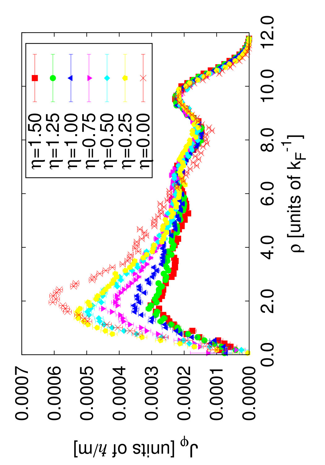 Figure 1
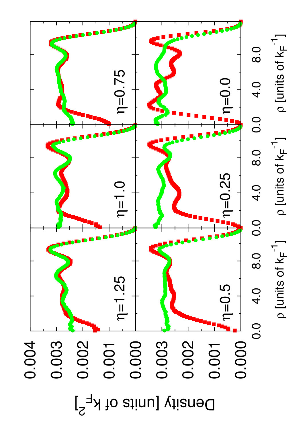 Figure 2
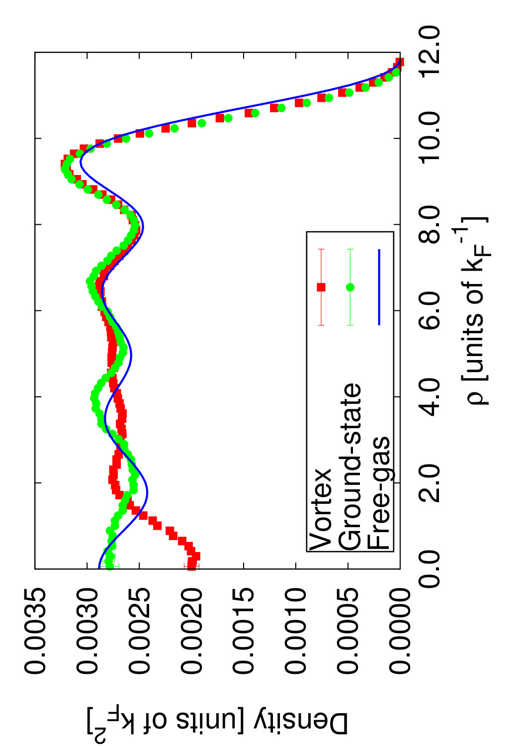 Figure 3
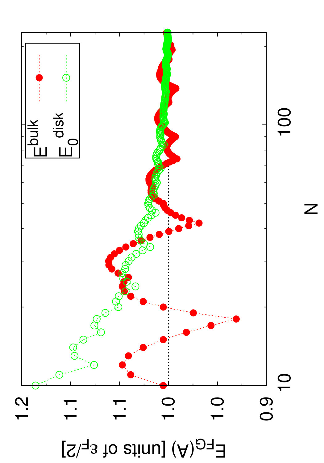 Figure 4
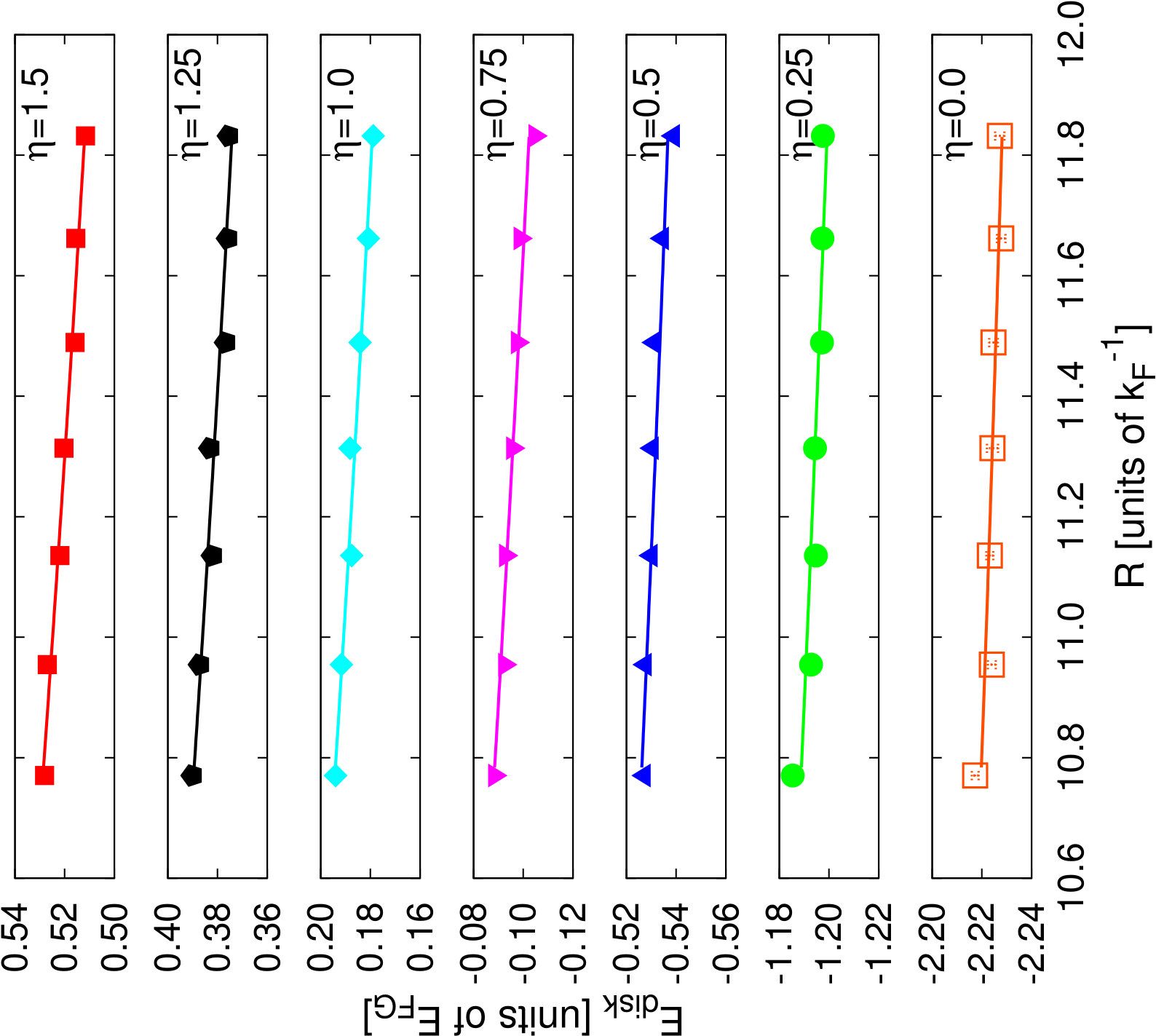 Figure 5
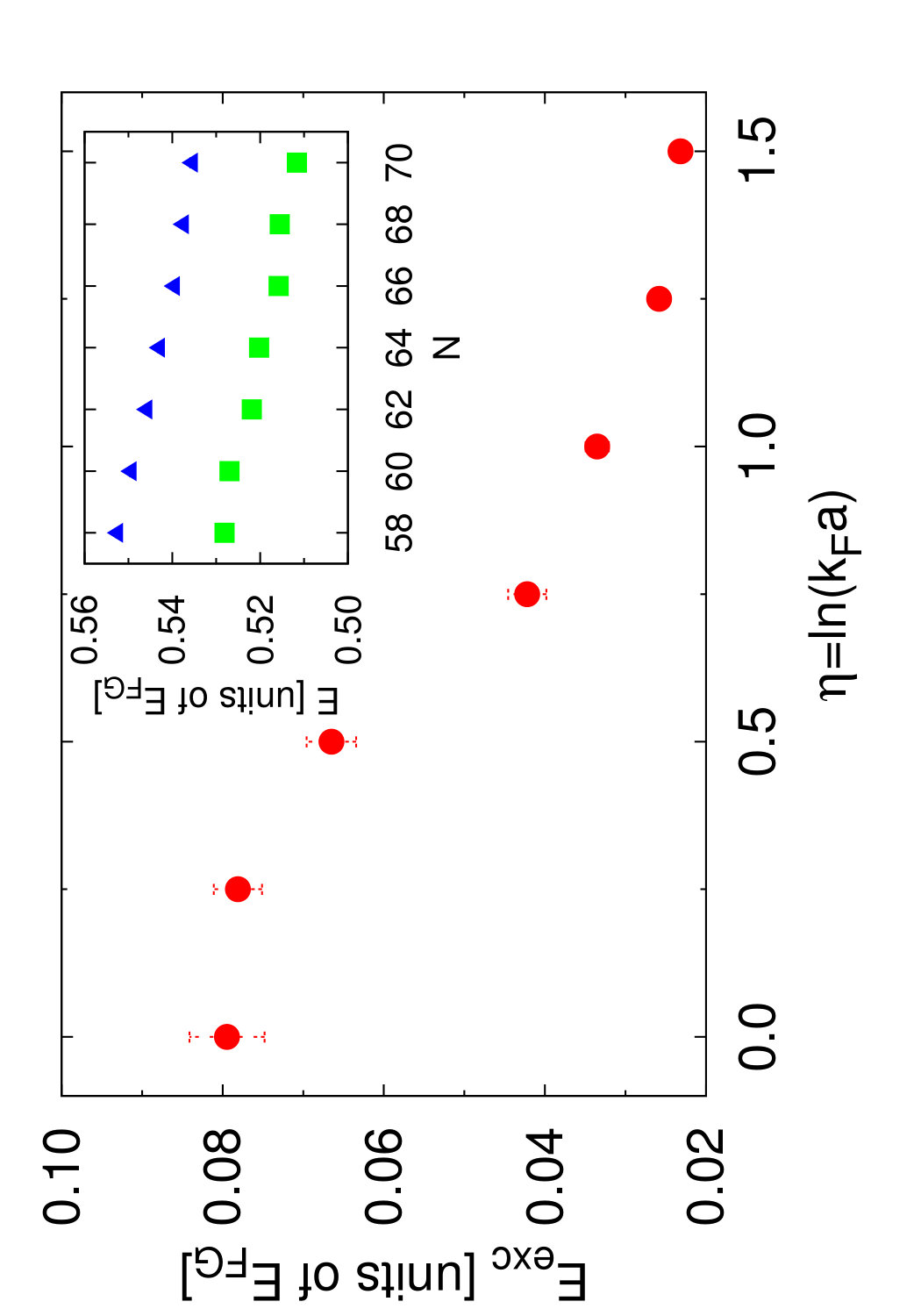 Figure 6
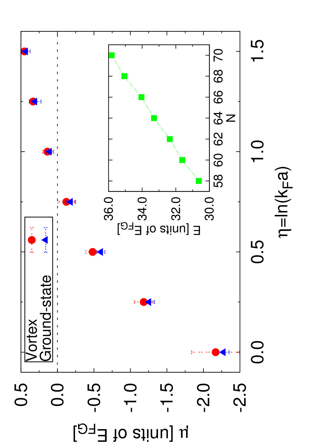 Figure 7
| [] | [] | [] | |
|---|---|---|---|
| 0.00 | -2.3740(3) | -2.32(3) | 16(2) |
| 0.25 | -1.3316(3) | -1.31(3) | 18(2) |
| 0.50 | -0.6766(2) | -0.65(2) | 18(1) |
| 0.75 | -0.2562(2) | -0.25(2) | 11(1) |
| 1.00 | -0.0233(2) | -0.03(1) | 11(1) |
| 1.25 | -0.2149(2) | -0.22(2) | 12(1) |
| 1.50 | -0.3523(2) | -0.34(1) | 13(1) |
Peer Reviews
No public reviews on file for this paper yet. If you reviewed it on a platform where reviews are public (OpenReview, ICLR, NeurIPS, ICML), you can paste yours below so the community can read it here.
Videos
No videos yet. Explain this paper in a talk, walkthrough, or lecture? Add one.
Core structure of two-dimensional Fermi gas vortices
in the BEC-BCS crossover region
Lucas Madeira
Department of Physics, Arizona State University, Tempe, Arizona 85287, USA
Stefano Gandolfi
Theoretical Division, Los Alamos National Laboratory, Los Alamos, New Mexico 87545, USA
Kevin E. Schmidt
Department of Physics, Arizona State University, Tempe, Arizona 85287, USA
Abstract
We report diffusion Monte Carlo results for the ground-state and vortex excitation of unpolarized spin-1/2 fermions in a two-dimensional disk. We investigate how vortex core structure properties behave over the BEC-BCS crossover. We calculate the vortex excitation energy, density profiles, and vortex core properties related to the current. We find a density suppression at the vortex core on the BCS side of the crossover and a depleted core on the BEC limit. Size-effect dependencies in the disk geometry were carefully studied.
pacs:
71.10.Ca, 05.30.Fk
I Introduction
The study of cold Fermi gases has proven to be a very rich research field, and the investigation of low-dimensional systems has become an active area in this context Giorgini et al. (2008); Bloch et al. (2008). Particularly, the two-dimensional (2D) Fermi gas has attracted much interest recently. It was the object of several theoretical investigations Randeria et al. (1989, 1990); Petrov et al. (2003); Martikainen and Törmä (2005); Tempere et al. (2007); Zhang et al. (2008), but its experimental realization, using a highly anisotropic potential, was a milestone in the study of these systems Martiyanov et al. (2010). Many other studies have been carried out since Orel et al. (2011); Makhalov et al. (2014). Quantum Monte Carlo (QMC) methods were successfully employed to compute several properties of the BEC-BCS crossover. These methods include diffusion Monte Carlo (DMC) Bertaina and Giorgini (2011); Galea et al. (2016), auxiliary-field quantum Monte Carlo Shi et al. (2015), and lattice Monte Carlo Anderson and Drut (2015); Rammelmüller et al. (2016); Luo et al. (2016). The fact that a fully attractive potential in 2D always supports a bound state, and the ability to vary the interaction strength over the entire BEC-BCS crossover regime offers rich possibilities for the study of these systems.
The presence of quantized vortices is an indication of a superfluid state in both Bose and Fermi systems. In three-dimensional (3D) systems, much progress has been made Bulgac and Yu (2003); Sensarma et al. (2006); Simonucci et al. (2013); Madeira et al. (2016), including the observation of vortex lattices in a strongly interacting rotating Fermi gas of 6Li Zwierlein et al. (2005). With the recent progress on the 2D Fermi gases, it seems natural to also extend the theoretical study of vortices to these systems. Interest is further augmented in 2D, where a Berezinksii-Kosterlitz-Thouless transition Berezinsky (1971); Kosterlitz and Thouless (1972) could take place at finite temperatures, and pairs of vortices and antivortices would eventually condense to form a square lattice Botelho and Sá de Melo (2006).
We are interested in how the properties of a vortex change over the BEC-BCS crossover. In this work we focus on ultracold atomic Fermi gases, but it is noteworthy that a duality is expected between neutron matter and superfluid atomic Fermi gases. In 3D, both ultracold atomic gases and low-density neutron matter exhibit pairing gaps of the order of the Fermi energy Carlson et al. (2013). Neutron-matter properties depend on the interaction strength and, unlike the Fermi atom gases, the possibility of microscopically tuning interactions of neutron-matter is not available. However, we can study neutron pairing by looking at the BCS side of the crossover Gezerlis and Carlson (2008, 2010). Vortex properties are also of significant interest in neutron matter De Blasio and Elgarøy (1999); Yu and Bulgac (2003) because a significant part of the matter in rotating neutron stars is superfluid, and vortices are expected to appear. Moreover, phases called nuclear pasta, where neutrons are restricted to 1D or 2D configurations, are predicted in neutron stars Ravenhall et al. (1983); Yu and Bulgac (2003).
We report properties of a single vortex in a 2D Fermi gas. We considered the ground-state to be a disk with hard walls and total angular momentum zero, and the vortex excitation corresponds to each fermion pair having angular momentum . Hopefully, our results will motivate experiments to increase our understanding of vortices in 2D Fermi gases.
This work is structured as it follows. In Sec. II we introduce the methodology employed. In Sec. II.1 we discuss aspects of finite-size fermionic systems, we briefly introduce 2D scattering in Sec. II.2, Sec. II.3 is devoted to the wave functions employed for the bulk, disk, and vortex systems, and we summarize the employed QMC methods in Sec. II.4. The results are presented in Sec. III. Sec. III.1 contains the ground-state energies in the disk geometry and discussions on size-effects. In Sec. III.2 we present the vortex excitation energy. The determination of the crossover region is done in Sec. III.3. Density profiles of the vortex and ground-state systems are shown in Sec. III.4. Properties of the vortex core are discussed in Sec. III.5. Finally, a summary of the work is presented in Sec. IV.
II Methods
Previous simulations of vortices in 3D bosonic systems, such as 4He, have often employed a periodic array of counter-rotating vortices, which enables the usage of periodic boundary conditions. In the 4He calculations of Ref. Sadd et al., 1997, the simulation cell consisted of 300 particles in four counter-rotating vortices. If we had employed a similar methodology, we would need the same number of fermion pairs, i.e., a system with 600 fermions. There are simulations of fermionic systems that have been performed with this number of particles, but the variance required for a detailed optimization is beyond the scope of this work. Instead, we considered a disk geometry similar to the one used in Ref. Ortiz and Ceperley (1995) for DMC simulations of the vortex core structure properties in 4He.
II.1 Finite-size systems
We are interested in the interacting many-body problem, but it is useful to first consider the non interacting case. In this section we compare the energy of finite-size 2D systems to the results in the thermodynamic limit.
First let us consider the case of fermions in a square of side with periodic boundary conditions. The single-particle states are plane waves , with wave vector
[TABLE]
The eigenenergies are , where is the mass of the fermion. At , all states with energy up to the Fermi energy , where is the Fermi wave number, are occupied. A shell structure arises from the fact that different combinations of and in Eq. (1) yield the same . The closed shells occur at total particle number . The free gas energy of a finite system with fermions, , is readily calculated by filling the lowest energy states described by Eq. (1). In the thermodynamic limit, which corresponds to and held constant, the energy per particle of the free gas is and .
Now let us consider the case of fermions in a disk of radius with a hard wall boundary condition, i.e., the wave function must vanish at . The single-particle states are
[TABLE]
where are the usual polar coordinates, is a normalization constant, are Bessel functions of the first kind, and is the -th zero of . The quantum number can take the values and . The corresponding eigenenergies are
[TABLE]
This system also presents a shell structure, due to the energy degeneracy of single-particles states with the same , with shell closures at total particle number . Notice that the energy levels of the bulk system are much more degenerate than the ones of the disk. In practice this means that more shells are needed to describe a disk with a given . The free gas energy for the disk, , can be calculated analogously to the bulk case using the energy levels of Eq. (3). The thermodynamic limit for this case corresponds to with held constant, and and go to the same expressions as the bulk ones.
The comparison between the free gas energy of finite systems in the bulk case and in the disk geometry is not immediate due to the presence of hard walls in the latter. In order to compare the free gas energy in both geometries, we define
[TABLE]
in which we separated the total energy into a bulk component, , and a surface term, the second term on the RHS. For further discussions on the functional form of the surface term, see Sec. III.1. Figure 1 shows and , with , at the same density. The value of , within a 0.2% error, was determined by fitting the data for to the functional form of Eq. (4).
The disk presents a considerably higher free gas energy, if compared to the bulk system, due to the presence of hard walls, but the difference between them is rapidly suppressed as we increase the particle number.
II.2 Scattering in 2D
Two-body scattering by a finite-range potential in 2D is described by the Schrödinger equation. We separate the solutions into radial and angular parts, the latter being a constant for -wave scattering. The two-body equation for an azimuthally symmetric (-wave) solution is
[TABLE]
where is the reduced mass of the system, and is the scattering energy. The scattering length and effective range can be easily determined from the solution of Eq. (5), , and its asymptotic form . We choose the solution
[TABLE]
and we match and , and their derivatives, outside the range of the potential.
In 2D, the low-energy phase shifts , , and effective range , are related by Khuri et al. (2009)
[TABLE]
where is the Euler-Mascheroni constant, and the effective range is defined as Adhikari et al. (1986)
[TABLE]
Equation (7) is often called the shape-independent approximation because it guarantees that a broad range of well-chosen potentials can be constructed to describe low-energy scattering. We consider the modified Poschl-Teller potential
[TABLE]
where and can be tuned to reproduce the desired and .
Bound-states occur for purely attractive potentials for any strength in 2D. If we continually increase the depth of , will eventually reach zero, and then it diverges to when a new bound-state is created. The binding energy of the pair is given by
[TABLE]
We chose values of and such that only one bound-state is present, and is held constant at 0.006 Galea et al. (2016). This choice guarantees that the systems studied in this work are in the dilute regime, since , where is of order of the interparticle spacing.
II.3 Wave functions
The BCS wave function, which describes pairing explicitly, has been successfully used in a variety of strongly interacting Fermi gases systems, such as: 3D Carlson et al. (2003) and 2D Galea et al. (2016) bulk systems, vortices in the unitary regime Madeira et al. (2016), two-component mixtures Gezerlis et al. (2009); Gandolfi (2014), and many other systems. This wave function, projected to a fixed number of particles (half with spin-up and half with spin-down), can be written as the antisymmetrized product Bouchaud, J.P. et al. (1988)
[TABLE]
where R is a vector containing the particle positions , stands for the spins , and is the pairing function, which is given by
[TABLE]
where we have explicitly included the spin part to impose singlet pairing. The assumed expressions for depend on the system being studied (see Secs. II.3.1, II.3.2, and II.3.3). Since neither the Hamiltonian or any operators in the quantities we calculate flip the spins, we adopt hereafter the convention of primed indexes to denote spin-down particles and unprimed ones to refer to spin-up particles. Equation (II.3) reduces to
[TABLE]
where the antisymmetrization is over spin-up and/or spin-down particles only. This wave function can be calculated efficiently as a determinant Gandolfi et al. (2009).
In addition to fully paired systems, it is also possible to simulate systems with unpaired particles Carlson et al. (2003), described by single particle states . For pairs, spin-up, and spin-down unpaired single particles states, , we can rewrite Eq. (II.3) as
[TABLE]
We also included a two-body Jastrow factor , , which accounts for correlations between antiparallel spins. It is obtained from solutions of the two-body Schrödinger’s equation
[TABLE]
with the boundary conditions and , where is a variational parameter, and is adjusted so that is nodeless. The total trial wave function is written as
[TABLE]
II.3.1 Bulk system
The assumed form of the pairing function for the bulk case is the same as Ref. Carlson et al. (2003),
[TABLE]
where are variational parameters, and contributions from momentum states up to a level are included. Contributions with are included through the function given by
[TABLE]
with
[TABLE]
where and , , and are variational parameters. This functional form of describes the short-distance correlation of particles with antiparallel spins. We consider = 0.5 , , and is adjusted so that at .
II.3.2 Disk
The pairing function for the disk geometry is constructed using the single-particle orbitals of Eq. (2). Each pair consists of one single-particle orbital coupled with its time-reversed state. This ansatz has been used before in the 3D system Madeira et al. (2016), a cylinder with hard walls, and the form presented here is analogous to that one if we disregard the components. We supposed the pairing function to be
[TABLE]
where the are variational parameters, and is a label for the disk shells, such that different states with the same energy are associated with the same variational parameter. The function is similar to employed in the bulk system, but we modify it to ensure the hard wall boundary condition is met,
[TABLE]
and has the same expression as the bulk case, Eq. (19).
II.3.3 Vortex
The vortex excitation is accomplished by considering pairing orbitals which are eigenstates of with eigenvalues . This is achieved by coupling single-particle states with angular quantum numbers differing by one. In this case we used pairing orbitals of the form
[TABLE]
where is a label for the vortex shells, and are variational parameters. The largest contribution is assumed to be from states with the same quantum number for the radial part Madeira et al. (2016). Equation (II.3.3) is symmetric under interchange of the prime and unprimed coordinates, as required for singlet pairing.
The function of Eq. (21) is not suited to describe the vortex state because it is an eigenstate of with angular momentum zero. We tried different functional forms that had the desired angular momentum eigenvalue, but none of them resulted in a significant lower total energy. Thus, we chose to employ only the terms in Eq. (II.3.3).
II.4 Quantum Monte Carlo
The Hamiltonian of the two-component Fermi gas is given by
[TABLE]
with , and given by Eq. (9). The DMC method projects the lowest energy state of from an initial state , obtained from variational Monte Carlo (VMC) simulations. The propagation, which is carried out in imaginary time , can be written as
[TABLE]
where is an energy offset. In the limit, only the lowest energy component survives
[TABLE]
The imaginary time evolution is given by
[TABLE]
where is the Green’s function associated with . The Green’s function contains two pieces, a diffusion term related to the kinetic operator, and a branching term related to the potential. We solve an importance sampled version of Eq. (26) iteratively, using the Trotter-Suzuki approximation to evaluate , which requires the time steps to be small. We circumvent the fermion-sign problem by using the fixed-node approximation, which restricts transitions across a chosen nodal surface Foulkes et al. (2001). Hence our estimates of energy expectation values are upper bounds.
We carefully optimized the trial wave function , since it is used in three ways: an approximation of the ground-state in the VMC calculations, as an importance function, and to give the nodal surface for the fixed-node approximation. The variational parameters 111See Supplemental Material at [url to be inserted by publisher] for the variational parameters of Eqs. (17), (II.3.2), and (II.3.3) in Eqs. (17), (II.3.2), and (II.3.3) were determined using the stochastic reconfiguration method Casula et al. (2004).
Expectation values of operators that do not commute with the Hamiltonian, for example the current and density, were calculated using extrapolated estimators Ceperley and Kalos (1986)
[TABLE]
where we combine the results of VMC and DMC runs.
III Results
We define the interaction strength . Large values of correspond to the BCS side of the crossover, while small are on the BEC side. We probed , which encompasses the crossover region (see Sec. III.3). For all systems the number density is , and .
III.1 Ground-state energy and size-effects
We used the pairing function of Eq. (17), and , to calculate the ground-state energy per particle of the bulk systems. Our results (see Table 1) are in agreement with previous DMC calculations Galea et al. (2016).
Previous DMC simulations of 2D Fermi gases found that is well suited to simulate bulk properties of systems in the region studied here Galea et al. (2016). However, the disk geometry presents more intricate size-dependent effects. We investigated how the ground-state energy depends on the disk radius . In the thermodynamic-limit, , the energy per particle should go to the bulk value. Since our system has hard walls, the energy has a dependence on the “surface” of the disk. Including this surface term, the energy per particle can be fit to
[TABLE]
where and are constants related to the bulk and surface terms, and can be viewed as a surface tension.
A few words about Eq. (28) are in order. The relation between the thermodynamic properties of a confined fluid and the shape of the container where it is confined has been an active field of study. Our choice was inspired by functional forms (see for example Ref. König et al. (2004)) where, aside from the constant term, thermodynamical properties are expressed as functions of the various curvatures of the container. The next correction to this functional form of the energy per particle would include a term proportional to . We found that the inclusion of such a term does not significantly improve our description of the ground- state energy.
In order to determine the number of particles necessary to simulate systems in the disk geometry, with controllable size effects, we performed simulations with , and all particles paired, i.e., only even values of . The dependence of with the system size was investigated by fitting our data using Eq. (28) for different intervals of or, equivalently, different intervals of .
We found that fitting the data for resulted in a good agreement between and , that is, we were able to separate the bulk portion of the energy from the hard wall contribution in the disk geometry. The resulting parameters of the fitting procedure are summarized in Table 1, and Fig. 2 shows the energy per particle as a function of for all interaction strengths studied in this work.
The values agree with the bulk energies within the error bars, except for and (however the differences between the values are less than 2% and 4%, respectively). As it can be seen in Table 1, the typical uncertainty in is of order 0.01 , independent of the interaction strength. Thus the relative error can be quite large for systems where the absolute value of the bulk energy is small, as it is observed for . This is an improvement if compared to a similar DMC calculation in 3D Madeira et al. (2016) which used the same procedure to calculate the ground-state energy per particle of a unitary Fermi gas, where the discrepancy between the result and the known bulk value was %.
We point out that this method is not intended to be a precise calculation of the bulk energy of these systems. Instead, it is a way for us to determine the minimum number of particles needed to simulate systems in the disk geometry with controllable size effects. If we had naively assumed that the same number of particles used in bulk calculations would suffice, , then we simply could not rely on the results. In our simulations with the discrepancies between and were as large as 50%, and in some cases the uncertainty in was bigger than the value itself. Results with are much more well-behaved, and they are within computational capabilities.
It is also noteworthy to mention that the energy contribution of the surface term, due to the presence of hard walls, is more significant for the BCS side than in the BEC limit (see the values in Table 1). This is expected, since the largest energy contribution in the BEC side should be from the binding energy of the pairs, Eq. (10), and they are smaller than the BCS pairs so that surface effects are smaller. One of our goals is to obtain the vortex excitation energy, which is the difference between the vortex and the ground-state energies. Since both systems have hard walls, we expect that the surface effects will tend to cancel.
III.2 Vortex excitation energy
The energy per particle of the vortex system is obtained using the pairing functions of Eq. (II.3.3). The vortex excitation energy is given by the difference between the energy of the vortex and ground-state systems, for the same number of particles. We performed simulations with and averaged the results.
In Fig. 3 we show the vortex excitation energy per particle as a function of the interaction strength. The energy necessary to excite the system to a vortex state increases as we move from the BCS to the BEC limit. The inset shows the vortex and ground-state energies per particle for , although the other interaction strengths display the same qualitative behavior.
III.3 Crossover region
In 2D, the BCS limit corresponds to and the BEC limit to , however unlike 3D where the unitarity is signaled by the addition of a two-body bound state, there is no equivalent effect with two-body sector in 2D. Nevertheless, we can determine the interaction strength for which we can add a pair to the system with zero energy cost. The chemical potential can be estimated as
[TABLE]
for each interaction strength, where the even number condition implies that all particles are paired. For each value of we used a finite difference formula to evaluate Eq. (29), for (see Fig. 4).
We found that at for the ground-state of the disk. Previous DMC simulations of 2D bulk systems Galea et al. (2016) found that the chemical potential changes sign at . Although the results differ, most probably due to the different geometry employed in this work, it is safe to assume that the interaction strength interval encompasses the BEC-BCS crossover region. The chemical potential of the vortex state is higher than the ground-state, as expected, thus is at a smaller interaction strength, .
III.4 Density profile
We calculated the density profile along the radial direction for both the vortex and ground-state systems. The normalization is such that
[TABLE]
where the integral is performed over the area of the disk. The results are obtained using the extrapolation procedure of Eq. (27), which combines both VMC and DMC runs. It is noteworthy to point out that, although the densities observed in VMC and DMC simulations differ, they are much closer than previous results in 3D Madeira et al. (2016). In that calculation it was needed to explicitly include a one-body term in the wave function to maximize the density overlap between DMC and VMC runs, whereas in this work no such term was employed.
Figure 5 shows the density profile of both the vortex and ground-state systems for and . The oscillations in the density profiles are much more pronounced than in a similar DMC calculation of a unitary Fermi gas in 3D Madeira et al. (2016). In this 3D calculation a cylindrical geometry was employed, with hard walls and periodic boundary conditions along the axis of the cylinder. The density profiles were obtained by averaging the results over the direction of the axis of the cylinder, we therefore expect more fluctuations in 2D where the particles are confined to a plane. For the ground-state, the density oscillations are surface effects. They are present in both the interacting and non-interacting systems, as it can be seen in Fig. 5.
In Fig. 6 we show the density profiles of the other interaction strengths studied in this work, . We found that the density depletion at the vortex core goes from 30% at to a completely depleted core at 0.25.
The regions close to the walls exhibit a characteristic behavior due to the hard wall condition we imposed, as it can be seen in Figs. 5 and 6. In order to estimate the number of particles outside this region, we can define the particle number a distance from the center of the disk as
[TABLE]
For the case of Figs. 5 and 6 where , if we set , is approximately between 40 and 45 for the ground-state, and between 35 and 40 for the vortex systems. Hence the number of particles in this regime is larger than the usual value of employed in bulk systems Galea et al. (2016).
Additionally, we performed simulations of the vortex systems with an odd number of particles, i.e., one unpaired particle was added to a fully paired system, Eq. (II.3) with , , and . We set its angular momentum to zero, Eq. (2) with and . In the BEC limit we observed a non-vanishing density at the center of the disk, which suggests that the unpaired particle fills the empty vortex core region. On the other hand, in the BCS limit the density close to the wall increased, while the density at the origin was unchanged. We chose a qualitative discussion of this phenomenon because the required variance for a detailed optimization is beyond the scope of this work. Future calculations should include quantities such as the one-body density matrix, which may contribute to an accurate quantitative approach.
III.5 Vortex core size
The probability current density operator can be written as
[TABLE]
where the velocity operator is . We are interested in the angular component as a function of the radial coordinate, , because the position of its maximum can be used as an estimate of the vortex core size, .
We followed the extrapolation procedure of Eq. (27). Figure 7 shows for and . The maximum of the current increases as we go from the BCS to the BEC limit, its value at the BEC side, , being more than twice at the BCS side, . The position of the maximum is between 1.7 and 1.8 at the BCS side of the crossover, i.e., ; at the BEC side, and 0.5, . The case moves away from the trend of a smaller core as we go from the BCS to the BEC limit, with . It is unclear if or depend on the disk radius , because the values are closely spaced for , and no significant difference was observed in the maximum as we varied . Nevertheless, the relative results contribute to understanding how the vortex core evolves over the BEC-BCS crossover.
The wave function that we employed for the vortex state is an eigenstate of the total angular momentum operator. Since this operator commutes with the Hamiltonian, the diffusion procedure does not change the eigenvalue of the state. In addition, the calculation of the probability current density operator allowed us to verify that the vortex corresponds to a total angular momentum state in a straightforward way. The angular momentum can be written as
[TABLE]
and the component of interest is
[TABLE]
In our definition of the probability current density operator, we divide by the number of particles , see Eq. (32). Thus, the evaluation of using Eq. (34) should yield . We verified that, for all interaction strengths, this is in agreement with our simulations.
IV Summary
We have investigated several properties of vortices in 2D Fermi gases over the BEC-BCS crossover region. We dedicated a considerable portion of this work to carefully understand and control size effects in the disk geometry, since it is very convenient to simulating a single vortex. Given that we were interested in the evolution of the properties in the BEC-BCS crossover, determining the crossover region was important to verify that the interaction strengths studied in this work span the crossover.
The vortex excitation energies and the density profiles are quantities that can be compared with experiments, once they become available. Interestingly, the observed density depletion of the vortex core goes from 30% at the BCS side, , to an empty core for , at the BEC limit. In 3D, Bogoliubov-de Gennes theory has been used to calculate the density suppression at the vortex core throughout the BEC-BCS crossover Bulgac and Yu (2003); Sensarma et al. (2006); Simonucci et al. (2013). Similar calculations in 2D could be compared to our findings 222After our calculations were done, it was pointed out to us that pseudogap phenomena occurring in 2D and 3D Fermi gases can be related in a universal way through a variable that spans the BEC-BCS crossover Marsiglio et al. (2015). Further studies are necessary to determine if this universality holds for other quantities, such as the density and the probability current density per particle. This would provide a very clean way of comparing 2D and 3D results.. Also, determining the probability current was essential to investigate the changes in the vortex core throughout the crossover region.
In 3D the interplay between experiments, theory, and simulations led to rapid advances in our comprehension of cold Fermi gases. Hopefully, our results will motivate experiments to increase our understanding of vortices in 2D Fermi gases.
Acknowledgements.
We would like to thank G. C. Strinati for useful discussions. This work was supported by the National Science Foundation under grant PHY-1404405. This work used the Extreme Science and Engineering Discovery Environment (XSEDE), which is supported by National Science Foundation grant number ACI-1053575. The work of S.G. was supported by the NUCLEI SciDAC program, the U.S. DOE under Contract No. DE-AC52-06NA25396, and the LANL LDRD program. We also used resources provided by NERSC, which is supported by the U.S. DOE under Contract No. DE-AC02-05CH11231.
The reference list from the paper itself. Each links out to its DOI / PubMed record.
- 1Giorgini et al. (2008) S. Giorgini, L. P. Pitaevskii, and S. Stringari, Rev. Mod. Phys. 80 , 1215 (2008) . · doi ↗
- 2Bloch et al. (2008) I. Bloch, J. Dalibard, and W. Zwerger, Rev. Mod. Phys. 80 , 885 (2008) . · doi ↗
- 3Randeria et al. (1989) M. Randeria, J.-M. Duan, and L.-Y. Shieh, Phys. Rev. Lett. 62 , 981 (1989) . · doi ↗
- 4Randeria et al. (1990) M. Randeria, J.-M. Duan, and L.-Y. Shieh, Phys. Rev. B 41 , 327 (1990) . · doi ↗
- 5Petrov et al. (2003) D. S. Petrov, M. A. Baranov, and G. V. Shlyapnikov, Phys. Rev. A 67 , 031601 (2003) . · doi ↗
- 6Martikainen and Törmä (2005) J.-P. Martikainen and P. Törmä, Phys. Rev. Lett. 95 , 170407 (2005) . · doi ↗
- 7Tempere et al. (2007) J. Tempere, M. Wouters, and J. T. Devreese, Phys. Rev. B 75 , 184526 (2007) . · doi ↗
- 8Zhang et al. (2008) W. Zhang, G.-D. Lin, and L.-M. Duan, Phys. Rev. A 78 , 043617 (2008) . · doi ↗