An integral-representation result for continuum limits of discrete energies with multi-body interactions
Andrea Braides, Leonard Kreutz

TL;DR
This paper establishes a mathematical framework for understanding the continuum limits of discrete lattice energies with complex multi-body interactions, ensuring the limit can be represented as an integral on Sobolev spaces.
Contribution
It provides a new compactness and integral representation theorem for atomistic lattice energies with multi-body interactions, including homogenization and applications to Jacobian determinants and Lennard-Jones energies.
Findings
Proved a compactness and integral representation theorem for lattice energies.
Derived conditions for the limit to be an integral on Sobolev spaces.
Applied results to multibody interactions like discrete Jacobian determinants and Lennard-Jones energies.
Abstract
We prove a compactness and integral-representation theorem for sequences of families of lattice energies describing atomistic interactions defined on lattices with vanishing lattice spacing. The densities of these energies may depend on interactions between all points of the corresponding lattice contained in a reference set. We give conditions that ensure that the limit is an integral defined on a Sobolev space. A homogenization theorem is also proved. The result is applied to multibody interactions corresponding to discrete Jacobian determinants and to linearizations of Lennard-Jones energies with mixtures of convex and concave quadratic pair-potentials.
Click any figure to enlarge with its caption.
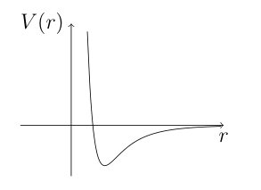 Figure 1
Peer Reviews
No public reviews on file for this paper yet. If you reviewed it on a platform where reviews are public (OpenReview, ICLR, NeurIPS, ICML), you can paste yours below so the community can read it here.
Videos
No videos yet. Explain this paper in a talk, walkthrough, or lecture? Add one.
Taxonomy
TopicsAdvanced Mathematical Modeling in Engineering · Composite Material Mechanics · Protein Structure and Dynamics
An integral-representation result for continuum limits of discrete energies with multi-body interactions
Andrea Braides
Dipartimento di Matematica, Università di Roma Tor Vergata
via della ricerca scientifica 1, 00133 Roma, Italy
e-mail: [email protected]
Leonard Kreutz
Gran Sasso Science Institute, Viale F. Crispi 7, 67100 L’Aquila, Italy
e-mail: [email protected]
Abstract
We prove a compactness and integral-representation theorem for sequences of families of lattice energies describing atomistic interactions defined on lattices with vanishing lattice spacing. The densities of these energies may depend on interactions between all points of the corresponding lattice contained in a reference set. We give conditions that ensure that the limit is an integral defined on a Sobolev space. A homogenization theorem is also proved. The result is applied to multibody interactions corresponding to discrete Jacobian determinants and to linearizations of Lennard-Jones energies with mixtures of convex and concave quadratic pair-potentials.
Keywords: lattice energies, discrete-to-continuum, multibody interactions, homogenization, Lennard-Jones energies
1 Introduction
This paper focuses on the passage from lattice theories to continuum ones in the framework of variational problems, such as for atomistic systems in Computational Materials Science (see e.g. [8]). For notational convenience we will state our results for energies defined on functions parameterized on a portion of (with values in ), but our assumptions may be immediately extended to more general lattices. For central interactions such energies may be written as
[TABLE]
where are points in the domain under consideration. We are interested in the behaviour of such an energy when the dimensions of the domain are much larger than the lattice spacing. In the discrete-to-continuum approach this can be done by approximation with a continuum energy obtained as a limit after a scaling argument. To that end, we introduce a small parameter (which, for the unscaled energy is the inverse of the linear dimension of the domain) and scale the energies as
[TABLE]
where now belong to a domain independent of , and the domain of is ; accordingly, we set . Both scalings, of the energy, and of the function, are important in this process and highlight that in this case we are regarding the energy as a volume integral ( being the volume element of a lattice cell) depending on a gradient ( being interpreted as a scaled difference quotient or discrete gradient). Other scalings are possible and give rise to different types of energies, depending on the form of , highlighting the multiscale nature of the problem. In the present context we focus on this particular “bulk” scaling (for an account of other scaling limits see [11, 12]).
The continuum approximation of is obtained by taking a limit as . This has been done in different ways, using a pointwise limit in [7] (where lattice functions are considered as restrictions of a smooth function to ) or a -limit in [2] (in this case lattice functions are extended as piecewise-constant functions and embedded in some common Lebesgue space) to obtain an energy of the form
[TABLE]
with domain a Sobolev space. We focus on the result of [2], which relies on the localization methods of -convergence (see [10] Chapter 12) envisaged by De Giorgi to deduce the integral form of the -limit from its behaviour both as a function of and . Conditions that allow to apply those methods are
(i) (coerciveness) growth conditions from below that allow to deduce that the limit is defined on some Sobolev space; e.g. that for nearest-neighbours and for all ;
(ii) (finiteness) growth conditions from above that allow to deduce that the limit is finite on the same Sobolev space; e.g. that for all , with some summability conditions on uniformly in ;
(iii) (vanishing non-locality) conditions that allow to deduce that the -limit is a measure in its dependence on . This is again obtained from some uniform decay conditions on the coefficients .
Hypotheses (i)–(iii) are sharp, in the sense that failure of any of these conditions may result in a -limit that cannot be represented as in (3). The result in [2] has been successful in many applications, among which the computation of optimal bounds for conducting networks [16], the derivation of nonlinear elastic energies from atomistic systems [2, 24], of their linear counterpart [19], and of -tensor theories from spin interactions [14], numerical homogenization [23], the analysis of the pile-up of dislocations [22], and others. Moreover, it has been extended to cover stochastic lattices [4] and dimension-reduction problems [1]. However, its range of applicability is restricted to pairwise interactions, which implies constraints on the possible energy densities. The main motivation of the present work is to overcome some of those limitations. More precisely, we focus on two issues:
the extension to the result to many-body interactions. In principle, a point in the lattice may interact with all other points in the domain . As a particular case, we may think of -body interactions corresponding to the minors of the lattice transformation (which is affine at the lattice level), such as the discrete determinant in two dimensions, which can be viewed as a three-point interaction. Some works in this direction are already present in the literature for particular cases [20, 25, 26];
the use of averaged growth conditions on the energy densities. Some lattice energies are obtained as an approximation of non-convex long-range interactions. As such, even when considering pair interactions, they may fail to satisfy coerciveness conditions for some . As an example we can think of the linearization of Lennard-Jones interactions, which gives concave quadratic energies for distant and . The coerciveness of the energy can nevertheless be recovered using the fast decay of the potential so that short-range convex interactions dominate long-range concave ones. In general, coerciveness can be obtained by substituting a growth conditions on each of the interactions with an averaged growth condition.
In order to achieve the greatest generality, we assume that energy densities may indeed depend on all points in . An energy density will describe the interaction of a point with all other points in the domain. This standpoint, already used in [13] for surface energies in a simpler setting (see also [18] in a one-dimensional setting), brings some notational complications (except for the case ) since it is convenient to regard each such function as defined on a different set . This complication is anyhow present each time that we consider more-than-two-body interactions. The energies are then defined as
[TABLE]
An important remark to make is that there are many ways to define energy densities giving the same . Note for example that for central interactions as above may be simply given by
[TABLE]
but the interactions may also be regrouped differently and in principle may include some with . This is important in order to allow that some be unbounded from below, up to satisfying a lower bound when considered together with the other interactions.
The set of hypotheses we are going to list for will allow to treat a larger class of energies than those of the form (2), but they must be stated with some care. The precise statements are given in Section 3. Here we give a simplified description as follows:
(o) (translational invariance in the codomain) for all , and vector . This condition is automatically satisfied for interactions depending on differences ;
(i) (coerciveness) the energy must be estimated from below by a nearest-neighbour pair energy and for all . This condition is less restrictive than the corresponding one for pair interactions since it refers to an already averaged energy density;
(ii) (Cauchy-Born hypothesis) we assume a polynomial upper bound for only when is linear. For energy densities as in (5) this in general rewritten in terms of as
[TABLE]
for all , and all matrices . This condition is in principle weaker than the finiteness property (ii) for pair interactions. Examining this condition separately goes in the direction of analyzing first pointwise convergence (as in [7]) and then -convergence;
(iii) (vanishing non-locality) we assume that if on a square of centre and side-length then
[TABLE]
( is identified with a piecewise-affine interpolation), where the rest is negligible as for bounded. Note that this condition is automatically satisfied with if the range of the interactions is finite, and can be deduced from the corresponding condition (iii) for central interactions;
(iv) (controlled non-convexity) a final condition must be added to ensure that the limit be a measure as a function of . For central interactions, this condition is hidden in the previous (i) and (ii), which imply a convex growth condition on ; more precisely a polynomial growth of the form
[TABLE]
This double inequality allows to use classical convex-combination arguments with cut-off functions even though may not be convex. In our case this compatibility with convex arguments must be required separately, and is formalized in condition (H5) in Section 3.1.
Under the conditions above we again deduce that -limits of energies are integral functionals as in (3) defined on a Sobolev space. The integrand can be described by a derivation formula, which is allowed by the study of suitably defined boundary-value problems. This derivation formula can also be used to prove a periodic-homogenization result. In the generality of energies possibly depending on the interaction of all points in some care must be used to define periodicity for the energy densities. In the case of finite-range interactions we require that in the interior of we have , where is periodic in . For infinite-range interactions the definition is given by approximation with periodic energy densities with finite-range interactions.
The paper is organized as follows. After some notation, in Section 3 we rigorously state the hypotheses outlined above and prove the main compactness and integral-representation theorem. Section 4 is devoted to formalizing and proving the convergence of Dirichlet boundary-value problems, which is used in the following Section 5 to state and derive a homogenization formula. Finally, Section 6 is devoted to examples. More precisely, we show how our hypotheses are satisfied by functions depending on discrete determinants and by a linearization of Lennard-Jones energies mixing convex and concave quadratic pair energy densities. Finally, in the same section we recover the result in [2] as a particular case of our main theorem.
2 Notation and preliminaries
We denote by an open and bounded subset of with Lipschitz boundary. We set to be the unit cube with sides orthogonal to the canonical orthonormal basis , and for we define . Moreover, for we set and . We set , , and for set and . For we write for the -dimensional Lebesgue measure of . For a vector we set
[TABLE]
We define for and
[TABLE]
the discrete difference quotient of at in direction .
For a function we set to be a constant depending on , the dimension and its domain of definition and which may vary from line to line.
Slicing. We recall the standard notation for slicing arguments (see [6]). Let , and let be the linear hyperplane orthogonal to . If and we define and . Moreover, if we set to .
-convergence. A sequence of functionals is said to -converge to a functional at as and we write if the following two conditions are satisfied:
- (i)
For every converging to in we have
- (ii)
There exists a sequence converging to in such that
We say that -converges to if for all .
If is a family of functionals indexed by a continuous parameter we say that -converges to as if for all we have that -converges to . We define the - and the - respectively by
[TABLE]
Note that the functionals , are lower semicontinuous and -converges to as if and only if .
Lattice functions. For we set We set .
Definition 2.1**.**
(Convergence of discrete functions) Functions can be interpreted by functions belonging to the space by setting (with slight abuse of notation) for all and
[TABLE]
where is the closest point of to (which is uniquely defined up to a set of measure [math]). We then say that in if the interpolations of converge to in .
Integral representation. We will use the following integral representation result (see [15]).
Theorem 2.2**.**
Let satisfy the following properties
- i)
(measure property) For every we have that is the restriction of a Radon measure to the open sets.
- ii)
(lower semicontinuity) For every we have that is weakly-* lower semicontinuous.*
- iii)
(bounds) For every it holds that
[TABLE]
- iv)
(translational invariance) For every and for every it holds .
- v)
(locality) For every and every such that a.e. in , we have that .
Then there exists a Carathèodory function such that
[TABLE]
for every .
- vi)
(translational invariance in ) if for every and for every such that we have that
[TABLE]
then does not depend on .
3 The main result
For all , we denote by the translation of the set with at the origin, and we consider a function . Let be defined by
[TABLE]
In this section we give hypothesis on the energy densities in order to ensure that the -limit of the energies defined in (7) be finite only on and there exists a Carathéodory function such that
[TABLE]
for all . A corresponding problem on the continuum is one of the first formalized in the theory of -convergence, when themselves are integral energies. In that approach integral functionals are interpreted as depending on a pair with u a Sobolev function and a subset of , when the integration is performed on only. The compactness property of -convergence then ensures that a -converging subsequence exits on a dense family of open sets by a simple diagonal argument. Showing that the dependence of the limit on the set variable is that of a regular measure, the convergence is extended to a larger family of sets, and an integral representation result can be applied. The type of conditions singled out in that case can be adapted to the discrete setting, taking into account that discrete energies are “nonlocal” in nature since they depend on the interactions of points at a finite distance. The locality of the limit energy must then be assured by a requirement of “vanishing nonlocality” as .
3.1 Hypotheses on the energy densities
A first requirement is that be invariant under addition of constants to ; namely
(H1) (translational invariance) for all we have
[TABLE]
for all , and .
A second requirement is that be finite if are a discretization of a function. In particular this should hold for affine functions.
(H2) (upper bound for the Cauchy-Born approximation) there exists , such that for every and we have
[TABLE]
for all and all .
We then also require that the limit domain be exactly functions, with . To that end a coerciveness condition should be imposed.
(H3) (equi-coerciveness) there exists such that
[TABLE]
for all and such that for all .
Next, we have to impose that the approximating continuum energy be local. Indeed, in principle discrete interactions are non-local, in that they take into account nodes of the lattice at a finite distance. This condition ensures that we can always find recovery sequences for a set that will not oscillate too much a finite distance away from . We expect the limit to depend on if only the interactions for small distances are relevant, or, in other words, if the decay of interactions is fast enough. This can be formulated otherwise: we may require that the overall effect of long-range interactions at a point decay sufficiently fast as follows.
(H4) (decaying non-locality) There exist , satisfying
[TABLE]
such that for all , satisfying for all we have
[TABLE]
The final condition is the most technical and derives from our requirement that the limit can be expressed in terms of an integral. This is the most restrictive in the vectorial case where convexity conditions have to be relaxed. A function is called a cut-off function if .
(H5) (controlled non-convexity) There exist and , satisfying
[TABLE]
such that for all and cut-off functions we have
[TABLE]
where
[TABLE]
Remark 3.1**.**
(observations on the assumptions) If condition (H1) fails we expect the limit not to be translational invariant anymore and if a integral representation exists it is expected to be of the form
[TABLE]
However, integral-representation theorems for non-translation-invariant functionals in general require restrictive hypotheses that should be added to (H2)–(H5).
If condition (H2) fails the -limit may not be finite on . Condition (H3) allows to estimate nearest-neighbour interactions centered in in terms of . Note that this estimate may still be true even if there are no interactions of the type taken into account by . Indeed if we may take
[TABLE]
If we assume a finite range of interactions and assume that the potential is well behaved in some sense condition (H4) is always satisfied and in the definition of the summation is only taken over . If condition (H4) fails the -limit may be non-local. Indeed there are examples where functionals of the form
[TABLE]
can be obtained as the -limit of energies of the form
[TABLE]
Note that (H1) is still satisfied. Condition (H5) mimics the so-called fundamental estimate in the continuum and ensures that the limit be subadditive as a set function. Note that this condition is satisfied for subadditive potentials with appropriate growth conditions. In particular, in Section 6.3 we show how the hypotheses above can be deduced from those in [2] in the case of pair potentials.
3.2 Compactness and integral representation
The goal of this section is to establish the proof of Theorem 3.2.
Theorem 3.2**.**
(Integral Representation)* Let be defined by (7), where satisfy (H1)–(H5). Then for every sequence of positive numbers converging to [math], there exists a subsequence and a Carathéodory function , quasiconvex in the second variable satisfying*
[TABLE]
with , such that -converges with respect to the -topology to the functional defined by
[TABLE]
Moreover, for any and any we have
[TABLE]
We will derive the proof of Theorem 3.2 as a consequence of some propositions and lemmas, which are fundamental in order to show that our limit functionals satisfies all the assumption of Theorem 2.2. In the next two proposition we show with the use of (H1)–(H5) that assumptions (ii) and (iii) of Theorem 2.2 are satisfied. Note that property (14) below allows to deduce weak lower-semicontinuity in even though we prove the -convergence of the discrete energies with respect to the strong -topology, so that assumption (ii) is satisfied.
Note that the proof of Proposition 3.3 is the same as the proof of Proposition 3.4 in [2]. We repeat it here only for completeness and the reader’s convenience.
Proposition 3.3**.**
Let satisfy (H3). If is such that , then and
[TABLE]
for some positive constant independent on and .
Proof.
Let and let in be such that . By (H3) we get
[TABLE]
For any , consider the sequence of piecewise-affine functions defined as follows
[TABLE]
Note that is a function of bounded variation and we will denote by the density of the absolutely continuos part of with respect to the Lebesgue measure. Moreover, for -a.e. the slices belong to . Note that, for any fixed , in for every . Moreover, since for , we get
[TABLE]
We now apply a standard slicing argument. By Fubini’s Theorem and Fatou’s Lemma for any we get
[TABLE]
Since, up to passing to a subsequence, we may assume that, for -a.e. in , we deduce that for -a.e. and
[TABLE]
Then by (15), we have
[TABLE]
Since, in particular, the previous inequality implies that
[TABLE]
thanks to the characterization of by slicing we obtain that and
[TABLE]
Letting , we get the conclusion. ∎
Proposition 3.4**.**
Let satisfy (H2),(H4) and (H5). We then have
[TABLE]
for some positive constant independent on and .
Proof.
We first show that the inequality holds for piecewise affine and then we recover the inequality for any by a density argument. Let be piecewise affine, that means
[TABLE]
where , with disjoint open simplices such that , . In the following, for such we construct , which agrees with on for all , on for all and close to we have that for some and independent on . The way we construct , it satisfies the same property close to the boundary so that (H5) or (H4) can be applied repeatedly. In we estimate the interactions separately with (H4).
Let
[TABLE]
and let . For choose inductively such that
[TABLE]
and define
[TABLE]
Set . We then have for all and strongly in and we claim that
[TABLE]
To this end define
[TABLE]
We have that strongly in and therefore
[TABLE]
We divide the energy into the energy of points which are far away from the boundary of all the and to the points which are close to some of the boundaries of :
[TABLE]
Now, note that for , and we have
[TABLE]
Moreover, note that for every we have that Using (H4) and (H2), noting that for and using the fact that for all (with slight abuse of notation we write for the discrete function as well as for the function defined in the continuum) we can estimate the first term by
[TABLE]
Taking the as taking into account (12) and using the dominated-convergence theorem we obtain
[TABLE]
Now let , that means for some . We prove
[TABLE]
for some constant depending on . Recall that , take and assume that we have proved already that
[TABLE]
we then prove that
[TABLE]
We either have in . Then by using , and (12) we obtain
[TABLE]
and we obtain (21). Now in the case that for some we use (H5) with as a cutoff function, as and the assumptions on we obtain
[TABLE]
with
[TABLE]
First, note that by (H2) and by we have
[TABLE]
and
[TABLE]
since . Now since for some we have that , on and . We therefore have
[TABLE]
for all and hence we have, splitting the sum into the summation over such that and the complement and using (22) we obtain
[TABLE]
for small enough, using (12). By summing over and, taking the maximum over in the inner sum and using (12) we obtain (21). If by (H2) and the definition of we have that
[TABLE]
and (20) follows. Now for we have that
[TABLE]
Therefore, using that and the dominated-convergence theorem, we have that
[TABLE]
By (18), (19) and (23) we obtain (17) and the claim follows. Now by the lower semicontinuity of we have
[TABLE]
Now for general we take piecewise affine such that strongly in and again by the lower semicontinuity of we have
[TABLE]
and the statement is proven. ∎
Proposition 3.5**.**
Let satisfy (H2)–(H5). Let and let be such that and . Then for any we have
[TABLE]
Proof.
Without loss of generality, we may suppose and finite. Let and converge to in and be such that
[TABLE]
and therefore
[TABLE]
By (H3) we have that
[TABLE]
for all . Since and converge to in , we have that
[TABLE]
Since there exists such that and converge to in and
[TABLE]
Take , such that , , , , , , and , and define ,. Now for , cut-off function we have
[TABLE]
Since , by (27), (31) and (32) we have that
[TABLE]
We can perform a similar construction for and therefore assume that an analogous bound to (33) holds also for . Moreover, since and converge to in we have that (29) and (30) hold with and . Now for , by (H4), it holds
[TABLE]
as well as a similar estimate for in . Set
[TABLE]
for any . Let be a cut-off function between and , with . Then for any consider the family of functions converging to in , defined as
[TABLE]
Given , then either , in which case either for and or and , or . In the first case, using (H4), we estimate
[TABLE]
In the second case, using (H4), we estimate
[TABLE]
Using (32) and the convexity of we have for and
[TABLE]
Now if we have that where . By (H5) we have that for such an it holds
[TABLE]
where
[TABLE]
Summing over and splitting into the two cases as described above, using (35)–(39), we have
[TABLE]
Note that . Therefore summing over , averaging and taking into account (25)–(29), (33) and Lemma 3.6 in [2], we get
[TABLE]
For any there exists such that
[TABLE]
Then, since still converges to in , by (40) and (41), letting we get
[TABLE]
Letting we obtain the claim. ∎
Proposition 3.6**.**
Let satisfy (H2)–(H5). Then for any and any we have
[TABLE]
Proof.
Since is an increasing set function, it suffices to prove
[TABLE]
In order to prove this, we define an extension of the functional to a functional defined on a bounded, smooth, open set such that
[TABLE]
for all and all such that in and therefore
[TABLE]
for all , and such that a.e. in . To this end we define by
[TABLE]
where is defined by
[TABLE]
with as in (15). Note that satisfies (H2)–(H5). Let , extended to . Let ; for find such that and
[TABLE]
Applying Proposition 3.5 with , , and we have and therefore
[TABLE]
Applying (42) to and we obtain
[TABLE]
The claim follows as . ∎
Proposition 3.7**.**
Let satisfy (H2)–(H5). Then for any and for any , such that a.e. in we have
[TABLE]
Proof.
Thanks to Proposition 3.6, we may assume that . We first prove
[TABLE]
Given there exist such that
[TABLE]
Let , be such that and in and
[TABLE]
Performing the same cut-off construction as in Proposition 3.5 we obtain a function converging to in such that for small enough we obtain
[TABLE]
for some . Taking we obtain
[TABLE]
Letting and we obtain the desired inequality. Exchanging the roles of and we obtain the other inequality. ∎
Proof of Theorem 3.2.
By the compactness property of -convergence there exists a subsequence of such that for any there exists
[TABLE]
(see [15] Theorem 10.3). Moreover, by Proposition 3.4 we have that
[TABLE]
for any . So it suffices to check that for every , satisfies all the hypothesis of Theorem 2.2 in [2]. In fact the superaditivity property of is conserved in the limit. Thus, as an consequence of Propositions (3.4)–(3.7) and thanks to De Giorgi-Letta Criterion (see [15]), hypotheses (i), (ii), (iii) hold true. Moreover, since is translationally invariant, hypothesis (iv) is satisfied and finally, by the lower semicontinuity property of -limit, also hypothesis (v) is fulfilled. ∎
4 Treatment of Dirichlet boundary data
In order to recover the limiting energy density we will establish the next lemma which asserts that our energies still converge if we suitably assign affine boundary conditions. From this, one is able to recover the value of in Theorem 3.2 by a blow-up argument. Given ,, and set
[TABLE]
For we define by
[TABLE]
Proposition 4.1**.**
Let satisfy (H1)–(H5). Let and be as in Theorem 3.2. For any and we set by
[TABLE]
Then for any and any we have that -converges with respect to the strong -topology to the functional .
Proof.
We only prove the statement for , the other cases being done analogously.
We first prove the - inequality. Let converge to in the -topology and be such that
[TABLE]
Since for all , and by (H3), we have that in and
[TABLE]
By the same reasoning as in Proposition 3.4 and . By Theorem 3.2 we therefore have
[TABLE]
To prove the - inequality we may first suppose that . Let converge to in and be such that
[TABLE]
Then by reasoning as in the proof of Proposition 3.6 given we can find and suitable cut-off functions with and such that for
[TABLE]
we have that converges to in and
[TABLE]
Using (H2) we have that for every it holds
[TABLE]
By the definition of the - we have that
[TABLE]
Letting we obtain the desired inequality. The general case follows by a density argument, approximating every function such that strongly in by functions such that and using the lower semicontinuity of the - as well as the continuity of with respect to the strong convergence in . ∎
Remark 4.2**.**
Let satisfy (H1)–(H5), and let be as in Theorem 3.2. For any and we have that
[TABLE]
since the functionals are coercive with respect to the strong -topology.
Note first that by extending the functional as in the proof of Proposition 3.6 we can assume that . Moreover, by the boundary conditions and by (H3) any sequence satisfying
[TABLE]
satisfies
[TABLE]
Then by the boundary conditions, Lemma 3.6 in [2] and the Riesz-Frechét-Kolmogorov Theorem there exists a function and a subsequence (not relabelled) that converges to . By Proposition 3.4 we have that . Moreover, in and therefore . This implies the coercivity.
5 Homogenization
We now consider the case where is periodic, though we have to explain what that means in our case, since the interaction energy at every point of the lattice may depend on the whole configuration of the state . This will be done by using a function , defined on the entire lattice. In order to define the energy density inside we assume that is approximated by finite-range interaction. More precisely, we suppose that there exist , -periodic, satisfying (H1)–(H3) uniformly in and
(4) (locality) For all and for all satisfying for all we have
[TABLE]
(5) (controlled non-convexity) There exist and , satisfying
[TABLE]
such that for all , and cut-off functions we have
[TABLE]
where
[TABLE]
(6) (closeness) There exist , satisfying
[TABLE]
such that For all and we have that
[TABLE]
(7) (monotonicity) For every , for every and for every we have
[TABLE]
The monotonicity property (7) may seem restrictive at a first sight, but it is not since by the positivity of and respectively we may reorder the interactions in a way that we keep only adding positive interactions with increasing .
For every we define by
[TABLE]
where and
[TABLE]
Note that (47) is well defined due to the locality property (4) and Moreover, satisfies (H1)–(H5). Those assumptions are made to avoid the dependence of on and still include infinite-range interactions.
Theorem 5.1**.**
Let satisfy (H1)–(H3) and (4)–(7) and be defined by (47). Then, -converges with respect to the strong -topology to the functional defined by
[TABLE]
where is given by
[TABLE]
where
[TABLE]
Remark 5.2**.**
Note that in Theorem 5.1 we have that the whole sequence -converges to the limit functional . We fix the boundary conditions of the admissible test functions on a boundary layer of width in order to have the boundary effects negligible while still being able to use a subadditivity argument in order to prove the existence of the limit in (48). Arguing as in the proof of Proposition 5.3 to show that the error goes to [math] when substituting with , and using the fact that the limit energy density is quasi-convex, we also have
[TABLE]
for all and all .
Proof.
By Theorem (3.2) for every sequence there exists a subsequence such that -converges to a functional such that for any and every we have
[TABLE]
By the Urysohn property of -convergence the theorem is proved if we show that does not depend on and . To prove the first claim it suffices to show that
[TABLE]
for all , and such that . By symmetry it suffices to prove
[TABLE]
By the inner-regularity property it suffices to prove for any
[TABLE]
Let be such that in and such that
[TABLE]
Let be a cut-off function such that
[TABLE]
For define by
[TABLE]
Thus by the periodicity assumption and the locality property we have that
[TABLE]
Therefore, we obtain
[TABLE]
In order to obtain that we note that by the lower semicontinuity with respect to the strong -topology and the coercivity of we obtain that is lower semicontinuous with respect to the weak -topology and hence is quasiconvex. By the growth properties of and Remark 4.2 we obtain for
[TABLE]
Where the last inequality follows from the next proposition. ∎
Proposition 5.3**.**
Let satisfy (H1)–(H3) and (4)–(7), and be defined by (47). Then
[TABLE]
for all .
Proof.
Without loss of generality, assume . We perform a change of variables
[TABLE]
Set . We obtain
[TABLE]
By the monotonicity property and (H2) we have that
[TABLE]
On the other hand, let be such that
[TABLE]
Now by (6) and setting we obtain , since , and
[TABLE]
We have that either in which case or . Now if , by [[2],Lemma 3.6] and (H2), we have that
[TABLE]
Now either , or , . We only deal with the first case, the second one being done analogously. Now if , by (H2) and using the boundary conditions, we have that
[TABLE]
If for every we choose a path by defining
[TABLE]
For this path it holds
[TABLE]
Now for every and for every we set
[TABLE]
We have that for , using for every and using Fubini’s Theorem we obtain
[TABLE]
Now if , using Fubini’s Theorem and (5), we obtain
[TABLE]
Now if , using Fubini’s Theorem and (5), we obtain
[TABLE]
If , using Fubini’s Theorem and (5), we obtain
[TABLE]
Now, dividing by , using (45),(5)–(5) and taking the limit as , we obtain
[TABLE]
It remains to show that the limit (48) exists and
[TABLE]
Since we have that
[TABLE]
On the other hand, for every , also , so that for we have
[TABLE]
Note that and therefore we are done if we can show that
[TABLE]
as and then . By the locality property (4) and the boundary conditions we have for all
[TABLE]
Using similar arguments as for (5)–(5) we obtain
[TABLE]
as and then and hence (55). We are done if we show that the limit in the definition of (48) exists. To this end set
[TABLE]
Let and let be such that . For any we have that and
[TABLE]
where the last term tends to [math] as , again using similar arguments as to prove (56). Noting that for every the function can also be used as a test function in the minimum on we obtain that
[TABLE]
Hence, we can assume that , and be such that
[TABLE]
We define by
[TABLE]
By the periodicity assumption and (H4) we have that
[TABLE]
Now, again using the same arguments as for (5)–(5), we obtain
[TABLE]
and therefore, noting that \lim\limits_{L\to\infty}\lim\limits_{S\to\infty}\frac{L^{N}}{S^{N}}\Big{\lfloor}\frac{S-\sqrt{S}}{L}\Big{\rfloor}^{N}=1, we get and the claim follows. ∎
6 Examples
6.1 The discrete determinant
An example of interactions that can be taken into account with our type of energies are discrete determinants. For we define
[TABLE]
where satisfy
[TABLE]
and satisfy
[TABLE]
(H1) follows, since does only depend on its difference quotients. Note that by Hadamard’s Inequality, the Geometric-Arithmetic mean Inequality and convexity we have
[TABLE]
Recall and therefore
[TABLE]
and by summing over (H2) follows. (H3) follows since we have exactly the coercivity term in the definition of and the first term is positive. For and in we have that
[TABLE]
Hence, by choosing
[TABLE]
(H4) follows. Setting
[TABLE]
we have that satisfies (13) and we have
[TABLE]
Note that for all cut-off functions and for all we have
[TABLE]
and hence (H5) follows by using the convexity of , and noting that
[TABLE]
A particular example could be and otherwise. More general our Theorems also apply to the case where we take functions of minors of as long as satisfies appropriate bounds.
6.2 The linearization of the Lennard-Jones potential
We assume . Our result is applicable to show an integral representation if the potential is the linearization of the Lennard-Jones potential, where the Lennard-Jones potential, pictured in Fig. 1, is defined by (up to renormalization)
[TABLE]
For open and smooth we define by
[TABLE]
In fact heuristically can be obtained by linearizing the Lennard-Jones Energy defined by
[TABLE]
where the set of admissible deformations should be close to the identity (neglecting the linear term in the expansion by the assumption that is an equilibrium point). The term
[TABLE]
may not be positive in general, due to the long-range part of the potential.
We may regroup the interactions of such that we have a positive potential satisfying the assumptions of our main theorem. For every we choose a path by defining
[TABLE]
For this path it holds
[TABLE]
For we define by
[TABLE]
and for we define
[TABLE]
Moreover, we define by
[TABLE]
and by
[TABLE]
We need to check that
[TABLE]
for some constant , and that satisfy (H1)–(H3) and (4)–(7). Note that for it holds
[TABLE]
By the definition of it is clear, that (H1), (H2) holds. To prove (H3) we have that for all and by Fubini’s Theorem we have that
[TABLE]
where \displaystyle N_{i,v}^{\xi}=\Big{\{}j\in\mathbb{Z}^{3}:\,\exists h\in\{1,\ldots,|\xi_{1}|\}\text{ such that }i=j_{h}\in\gamma^{\xi}_{j}\text{ and }e_{n(h)}=v\Big{\}}. Note that for such that we have and otherwise. Hence, using the monotonicity of for and the fact that and using the fact that , we obtain
[TABLE]
Hence, we obtain (59) and with that (H3). (4) and (7) follow from the definition of and . Setting
[TABLE]
and if . Using (60) and (6.2) we obtain (45) and
[TABLE]
with defined in () with defined by (62). By the non-negativity of it follows (). Setting
[TABLE]
and if , using (60) and (6.2) we obtain (44). We have that
[TABLE]
and hence we obtain (6). Applying Theorem 5.1 we obtain the -convergence of to a functional given by
[TABLE]
where is given by
[TABLE]
6.3 Pair interactions: the Alicandro-Cicalese theorem
The compactness theorem can be applied to the special case of pair potentials where takes only into account the pair interactions of that point with every other point , that means it is of the form
[TABLE]
with satisfying
- (i)
for all , and .
- (ii)
for all , and , where
[TABLE]
(H1) follows since for each the interaction depend only on . (H2) follows from (64) and (ii). (H3) follows from (i). (H4) follows if we choose
[TABLE]
Let such that in . Then, using the positivity of and (ii), we obtain
[TABLE]
and therefore (H4) follows. Setting
[TABLE]
we have that
[TABLE]
and again for a cut-off function and (H5) follows by using (57), the convexity of and (58).
The reference list from the paper itself. Each links out to its DOI / PubMed record.
- 1[1] R. Alicandro, A. Braides and M. Cicalese. Continuum limits of discrete thin films with superlinear growth densities. Calculus of Variations and Partial Differential Equations 33.3 (2008): 267-297.
- 2[2] R. Alicandro and M. Cicalese. A general integral representation result for continuum limits of discrete energies with superlinear growth. SIAM journal on mathematical analysis 36.1 (2004): 1-37.
- 3[3] R. Alicandro and M. Cicalese. Variational analysis of the asymptotics of the XY model. Archive for rational mechanics and analysis 192.3 (2009): 501-536.
- 4[4] R. Alicandro, M. Cicalese and A. Gloria. Integral representation results for energies defined on stochastic lattices and application to nonlinear elasticity. Archive for rational mechanics and analysis 200.3 (2011): 881-943.
- 5[5] R. Alicandro and M.S. Gelli. Local and nonlocal continuum limits of Ising-type energies for spin systems. SIAM journal on mathematical analysis 49 (2016): 895–931.
- 6[6] L. Ambrosio, N. Fusco and D. Pallara. Functions of Bounded Variation and Free Discontinuity Problems . (Oxford: Clarendon Press, 2000).
- 7[7] X. Blanc, C. Le Bris and P.L. Lions. From molecular models to continuum models. Archive for Rational Mechanics and Analysis 332 (2002): 949–956.
- 8[8] X. Blanc, C. Le Bris and P.L. Lions. Atomistic to continuum limits for computational materials science. ESAIM: Mathematical Modelling and Numerical Analysis 41.2 (2007): 391-426.