Evolution of Galactic Outflows at $z\sim0$-$2$ Revealed with SDSS, DEEP2, and Keck spectra
Yuma Sugahara, Masami Ouchi, Lihwai Lin, Crystal L. Martin, Yoshiaki, Ono, Yuichi Harikane, Takatoshi Shibuya, Renbin Yan

TL;DR
This study analyzes galactic outflows from $z o0$ to 2$ using stacked optical spectra, revealing that outflow velocities and mass loading factors increase with redshift, consistent with galaxy evolution models and high gas fractions.
Contribution
First systematic measurement of outflow velocity and mass loading factor evolution from $z o0$ to 2$ using homogeneous stacked spectra and multi-component absorption line fitting.
Findings
Outflow velocities increase by 0.05-0.3 dex from $z o0$ to 2$ at fixed SFR.
Mass loading factors $ o$ increase with redshift as $(1+z)^{1.2 extpm0.3}$.
Results align with galaxy size evolution and high gas fractions at high redshift.
Abstract
We conduct a systematic study of galactic outflows in star-forming galaxies at - based on the absorption lines of optical spectra taken from SDSS DR7, DEEP2 DR4, and Keck Erb et al. We carefully make stacked spectra of homogeneous galaxy samples with similar stellar mass distributions at -, and perform the multi-component fitting of model absorption lines and stellar continua to the stacked spectra. We obtain the maximum (v_\rm{max}) and central (v_\rm{out}) outflow velocities, and estimate the mass loading factors (), a ratio of the mass outflow rate to the star formation rate (SFR). Investigating the redshift evolution of the outflow velocities measured with the absorption lines whose depths and ionization energies are similar (Na I D and Mg I at -; Mg II and C II at -), we identify, for the first time, that the average value of…
Click any figure to enlarge with its caption.
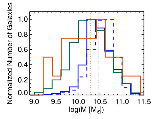 Figure 1
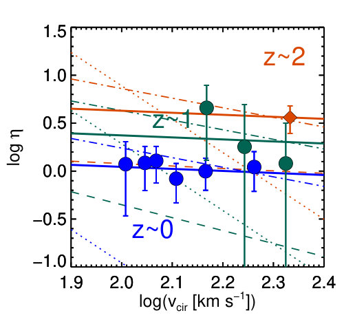 Figure 2
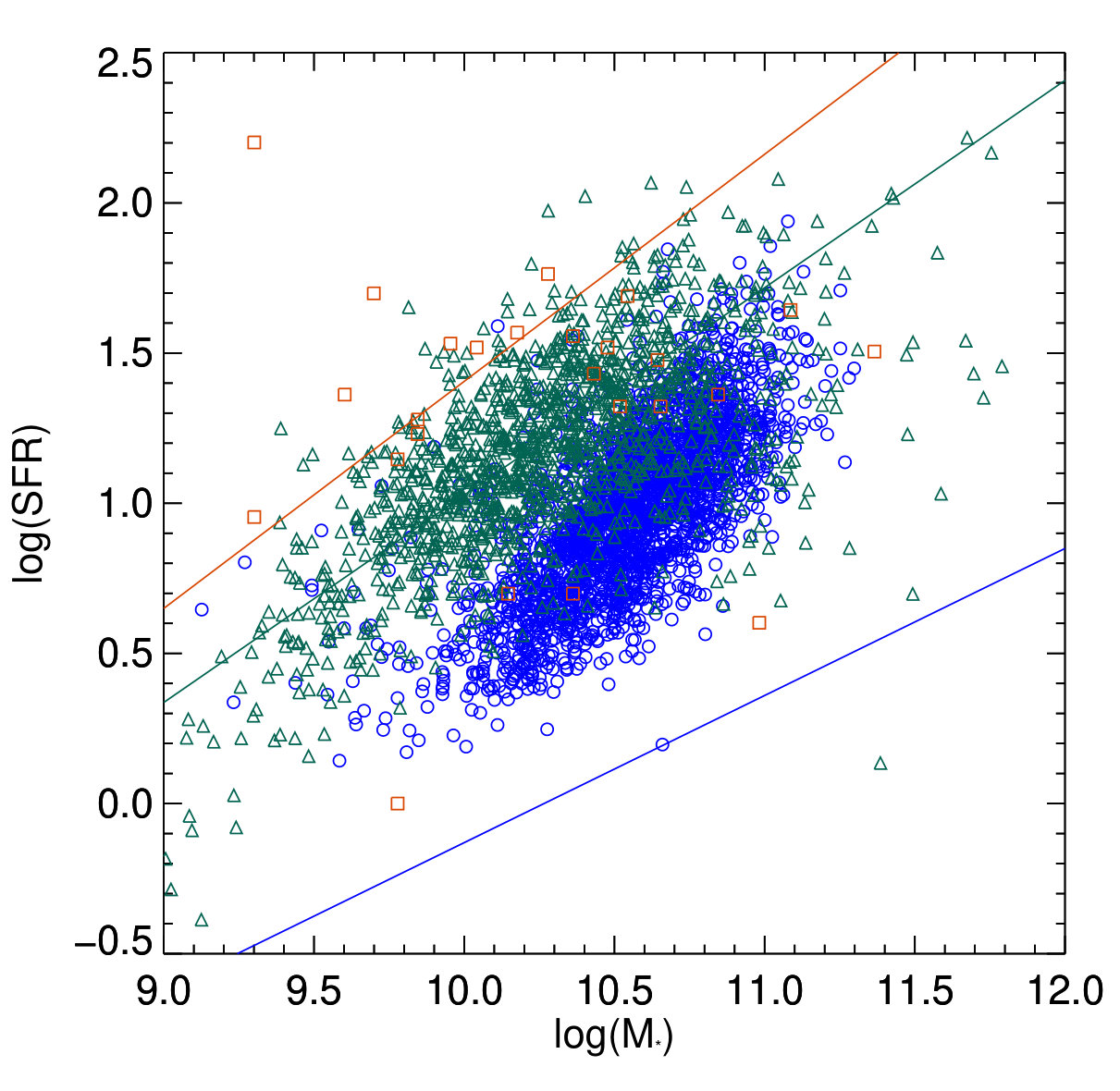 Figure 3
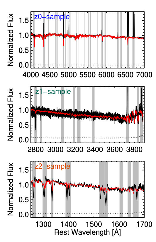 Figure 4
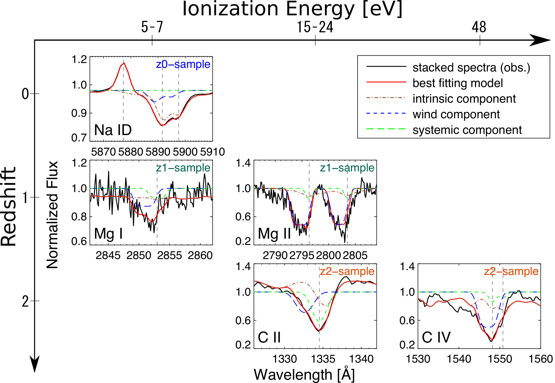 Figure 5
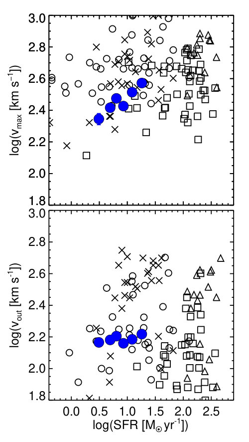 Figure 6
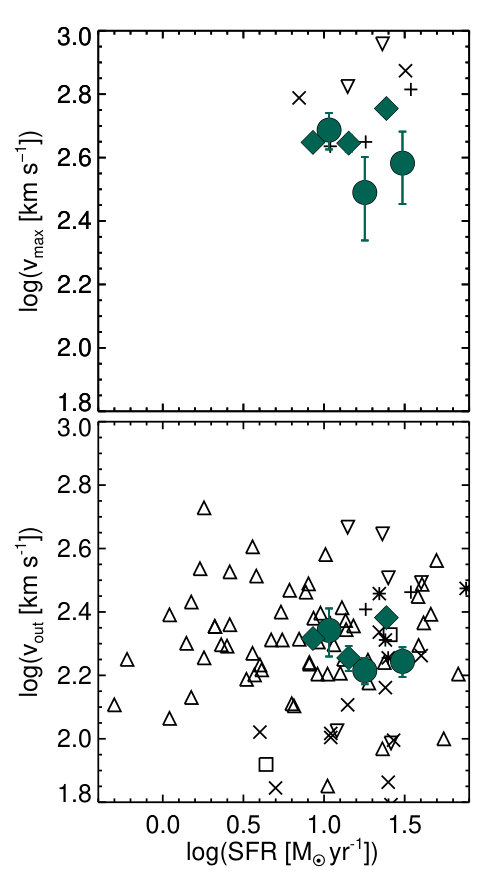 Figure 7
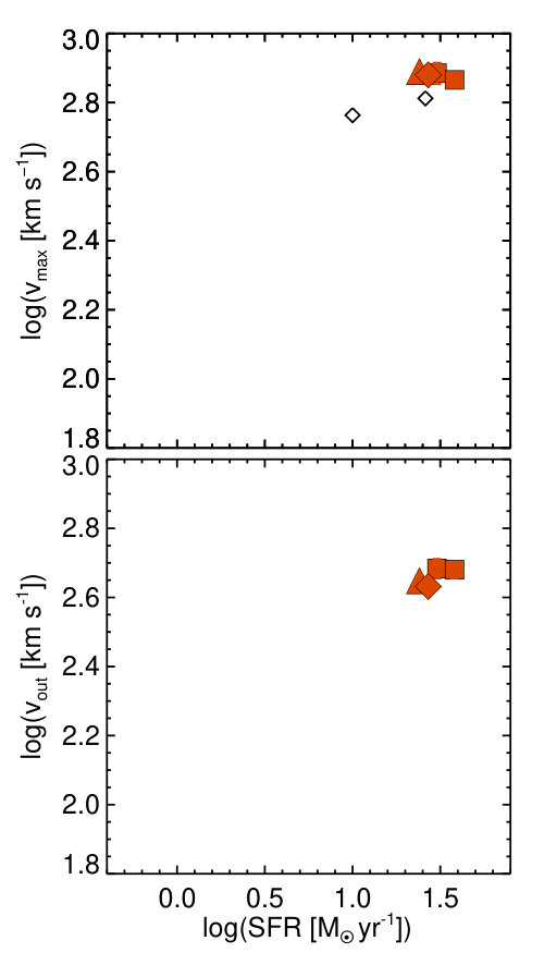 Figure 8
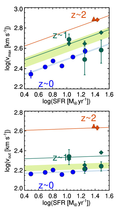 Figure 9
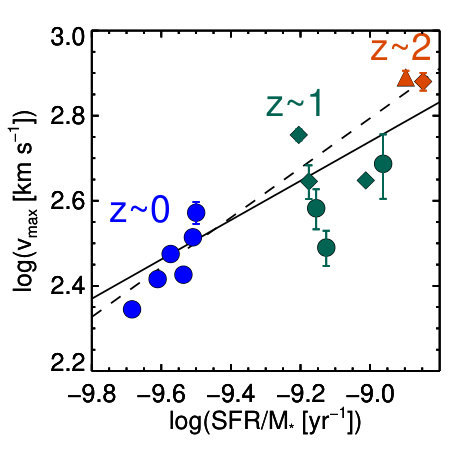 Figure 10
| sample | line | number | SFR | |||||
|---|---|---|---|---|---|---|---|---|
| () | () | () | () | |||||
| 0-sample | Na i D | 126 | 0.064 | 0.49 | 10.2 | 146 5.2 | 221 18 | 1.2 0.84 |
| Na i D | 113 | 0.075 | 0.69 | 10.3 | 152 4.4 | 261 12 | 1.2 0.59 | |
| Na i D | 109 | 0.085 | 0.80 | 10.4 | 160 4.5 | 299 11 | 1.3 0.53 | |
| Na i D | 138 | 0.11 | 0.93 | 10.5 | 144 4.3 | 267 11 | 0.83 0.37 | |
| Na i D | 141 | 0.13 | 1.1 | 10.6 | 153 4.3 | 327 10 | 1.0 0.37 | |
| Na i D | 123 | 0.14 | 1.3 | 10.8 | 165 9.7 | 373 20 | 1.1 0.49 | |
| 1-sample | Mg i | 662 | 1.4 | 1.0 | 9.99 | 220 38 | 486 64 | 4.6 3.3 |
| Mg i | 394 | 1.4 | 1.3 | 10.4 | 164 16 | 309 91 | 1.8 3.2 | |
| Mg i | 277 | 1.4 | 1.5 | 10.6 | 175 19 | 382 98 | 1.2 2.0 | |
| Mg ii | 662 | 1.4 | 1.0 | 9.99 | 207 5.0 | 445 9 | … | |
| Mg ii | 394 | 1.4 | 1.3 | 10.4 | 180 16 | 442 27 | … | |
| Mg ii | 277 | 1.4 | 1.5 | 10.6 | 241 7.1 | 569 12 | … | |
| 2-sample | C ii | 25 | 2.2 | 1.4 | 10.3 | 428 20 | 759 20 | 3.6 1.2 |
| C iv | 25 | 2.2 | 1.4 | 10.3 | 445 16 | 776 16 | … |
Peer Reviews
No public reviews on file for this paper yet. If you reviewed it on a platform where reviews are public (OpenReview, ICLR, NeurIPS, ICML), you can paste yours below so the community can read it here.
Videos
No videos yet. Explain this paper in a talk, walkthrough, or lecture? Add one.
Evolution of Galactic Outflows at –2 Revealed with SDSS, DEEP2, and Keck spectra
Yuma Sugahara11affiliationmark: 22affiliationmark: , Masami Ouchi11affiliationmark: 33affiliationmark: , Lihwai Lin44affiliationmark: , Crystal L. Martin55affiliationmark: , Yoshiaki Ono11affiliationmark: , Yuichi Harikane11affiliationmark: 22affiliationmark: ,
Takatoshi Shibuya11affiliationmark: , and Renbin Yan66affiliationmark:
1Institute for Cosmic Ray Research, The University of Tokyo, 5-1-5 Kashiwanoha, Kashiwa, Chiba 277-8582, Japan; [email protected]
2Department of Physics, Graduate School of Science, The University of Tokyo, 7-3-1 Hongo, Bunkyo, Tokyo, 113-0033, Japan
3 Kavli Institute for the Physics and Mathematics of the Universe (WPI), The University of Tokyo, 5-1-5 Kashiwanoha, Kashiwa, Chiba 277-8583, Japan
4 Institute of Astronomy & Astrophysics, Academia Sinica, Taipei 106, Taiwan (R.O.C.)
5 Department of Physics, University of California, Santa Barbara, CA, 93106, USA
6 Department of Physics and Astronomy, University of Kentucky, 505 Rose St., Lexington, KY 40506-0057, USA
Abstract
We conduct a systematic study of galactic outflows in star-forming galaxies at –2 based on the absorption lines of optical spectra taken from SDSS DR7, DEEP2 DR4, and Keck Erb et al. We carefully make stacked spectra of homogeneous galaxy samples with similar stellar mass distributions at –2, and perform the multi-component fitting of model absorption lines and stellar continua to the stacked spectra. We obtain the maximum () and central () outflow velocities, and estimate the mass loading factors (), a ratio of the mass outflow rate to the star formation rate (SFR). Investigating the redshift evolution of the outflow velocities measured with the absorption lines whose depths and ionization energies are similar (Na i D and Mg i at –; Mg ii and C ii at –), we identify, for the first time, that the average value of () significantly increases by 0.05–0.3 dex from to at a given SFR. Moreover, we find that the value of increases from to 2 by at a given halo circular velocity , albeit with a potential systematics caused by model parameter choices. The redshift evolution of () and is consistent with the galaxy-size evolution and the local velocity-SFR surface density relation, and explained by high-gas fractions in high-redshift massive galaxies, which is supported by recent radio observations. We obtain a scaling relation of for in our galaxies that agrees with the momentum-driven outflow model () within the uncertainty.
Subject headings:
galaxies: formation — galaxies: evolution — galaxies: ISM — galaxies: kinematics and dynamics
††slugcomment: ApJ in press
1. INTRODUCTION
The large scale structure of the universe is well explained by gravitational interactions based on the Lambda cold dark matter (CDM) model (e.g., Springel et al. 2005). However, we need additional models to explain small scale structures like galaxies, because these small scales are significantly affected by the baryon physics, such as gas cooling, radiation heating, star formation, and supernovae (SNe). In fact, there is a notable discrepancy between the shapes of the halo mass function predicted by numerical simulations of CDM model and the galaxy stellar mass function confirmed by observations (e.g., Somerville & Davé 2015). Theoretical studies suggest that this problem of the discrepancy is resolved by the feedback processes that regulate the star formation. Understanding the feedback processes is key to galaxy formation and evolution.
Galactic outflows driven by star-forming activities are one of the plausible sources of the feedback processes. The cold gas is accelerated by the starburst or the SNe, and carried even to the outside of the halos. The lack of the cold gas thus quenches the star formation in the galaxies. Although the outflows make an impact on the star formation activity, their physical mechanisms are still poorly known. Theoretical studies propose some physical processes to launch the galactic outflows such as the thermal pressure of the core-collapse SNe (e.g., Larson 1974; Chevalier & Clegg 1985; Springel & Hernquist 2003), the radiation pressure of the starburst (e.g., Murray et al. 2005; Oppenheimer & Davé 2006), and the cosmic ray pressure (e.g., Ipavich 1975; Breitschwerdt et al. 1991; Wadepuhl & Springel 2011).
Since the outflow scale is very small in cosmological simulations, major numerical simulations carry out the outflows as subgrid physics. (see Somerville & Davé 2015, for a recent review). On the other hand, some recent simulations employ the explicit thermal feedback generated by SNe with no outflows in subgrid physics, and describe the relation between the outflow and galaxy properties (Schaye et al. 2015; Muratov et al. 2015; Barai et al. 2015). Muratov et al. (2015) and Barai et al. (2015) predict that outflow properties evolve towards high redshift based on their numerical models. Mitra et al. (2015) support the evolution of the outflow properties with their analytic model including empirical relations.
Optical and ultra-violet (UV) observations investigate the galactic outflows with emission lines (Lehnert & Heckman 1996a, b; Heckman et al. 1990; Martin 1998), and absorption lines (Heckman et al. 2000; Schwartz & Martin 2004; Martin 2005; Rupke et al. 2005a, b; Tremonti et al. 2007; Martin & Bouché 2009; Grimes et al. 2009; Alexandroff et al. 2015) that are found in the spectra of outflow galaxies (“down-the-barrel” technique). Particularly, the absorption lines are used to probe outflow velocities of star-forming galaxies at (Chen et al. 2010; Chisholm et al. 2015, 2016), at (Sato et al. 2009; Weiner et al. 2009; Martin et al. 2012; Kornei et al. 2012; Rubin et al. 2014; Du et al. 2016), and at (Shapley et al. 2003; Steidel et al. 2010; Erb et al. 2012; Law et al. 2012; Jones et al. 2013; Shibuya et al. 2014). Moreover, absorption lines of background quasars are used to study the galactic outflows of foreground galaxies on the sight lines of the background quasars (Bouché et al. 2012; Kacprzak et al. 2014; Muzahid et al. 2015; Schroetter et al. 2015, 2016).
Despite many observations in a wide redshift range, it is challenging to study evolution of outflow velocities because of possible systematic errors included in different redshift samples. The literature uses various procedures to measure outflow velocities, such as non-parametric (Weiner et al. 2009; Heckman et al. 2015), one-component (Steidel et al. 2010; Kornei et al. 2012; Shibuya et al. 2014; Du et al. 2016), and two-component methods (Martin 2005; Chen et al. 2010; Martin et al. 2012; Rubin et al. 2014). Moreover, we should compare the samples of galaxies in the same stellar mass and star formation rate (SFR) ranges because the outflow properties depend on the stellar mass and SFR (i.e., Weiner et al. 2009; Erb et al. 2012; Heckman et al. 2015). Although Du et al. (2016) compare outflow velocities of star-forming galaxies at with those at that are derived with the same procedure, Du et al. (2016) cannot make similar galaxy samples at and due to the lack of stellar mass measurements.
In this paper, we investigate the redshift evolution of galactic outflows found in the star-forming galaxies. We use spectra of galaxies at , 1, and 2 drawn from the Sloan Digital Sky Survey (SDSS; York et al. 2000), the Deep Evolutionary Exploratory Probe 2 (DEEP2) Galaxy Redshift Survey (Davis et al. 2003, 2007; Newman et al. 2013), and Erb et al. (2006a, b), respectively. The combination of these data sets enables us to study the redshift evolution of outflow velocities based on the samples of star-forming galaxies with the same stellar mass and SFR ranges. Section 2 presents three samples of star-forming galaxies and our methods for spectrum stacking. We explain our analysis to estimate properties of outflowing gas in Section 3. We provide our results of the outflow velocities in Section 4, and discuss the redshift evolution of the outflow properties in Section 5. Section 6 summarizes our results. We calculate stellar masses and SFRs by assuming a Chabrier (2003) initial mass function (IMF). We adopt a CDM cosmology with , , , , and throughout this paper, which are the same parameters as those used in Behroozi et al. (2013). All transitions are referred to by their wavelengths in vacuum. Magnitudes are in the AB system.
2. DATA & SAMPLE SELECTION
To study galactic outflows, we construct three samples at –2. A sample is drawn from the SDSS Data Release 7 (DR7; Abazajian et al. 2009), a sample is drawn from the DEEP2 Data Release 4 (DR4; Newman et al. 2013), and a sample is drawn from Erb et al. (2006a). Each spectrum of galaxies in three samples does not have the signal-to-noise ratio (S/N) high enough for analysis of absorption lines. We therefore produce high S/N composites by stacking the spectra. In this section, we describe each sample and explain the method of the spectrum stacking. Properties of the stacked spectra are listed in Table 1. We discuss the selection biases between three samples in Section 4.2.
2.1. Galaxies at
We select star-forming galaxies at from the SDSS DR7 (Abazajian et al. 2009) main galaxy sample (Strauss et al. 2002). The spectra of these galaxies have a mean spectral resolution of , a dispersion of , and a wavelength coverage spanning between 3800 and 9200 Å. These spectra are taken with fibers of a 3 diameter, that are placed at the center of the galaxies. The SDSS imaging data are taken through a set of , , , , and filters (Fukugita et al. 1996) using a drift-scanning mosaic CCD camera (Gunn et al. 1998).
Since our targets are active star-forming disk galaxies, we need some galaxy properties for sample selection. The galaxy properties are mainly taken from the MPA/JHU galaxy catalog111 The MPA/JHU galaxy catalog is available at http://www.mpa-garching.mpg.de/SDSS/DR7. Systemic redshifts are derived with observed spectra and a linear combination of the galaxy template spectra. Because this measurement may be affected by blueshifted absorption that outflowing gas produce, we compare in the MPA/JHU catalog with redshifts measured by fitting H emission lines alone with a Gaussian function. We find that the difference of the two redshifts is typically and negligible. Stellar masses are obtained by the fitting to the photometry (Kauffmann et al. 2003; Salim et al. 2007). SFRs within the fiber () are measured from the extinction-corrected emission-line flux, and total SFR are estimated by applying aperture correction with the photometry outside the fiber (Brinchmann et al. 2004). For our study, stellar masses and SFRs are converted from a Kroupa (2001) IMF to a Chabrier (2003) IMF with a correction factor of 0.93. SFR surface densities are defined as /, where is the physical length corresponding to the SDSS 1.5 aperture radius. The MPA/JHU catalog also includes the emission- and absorption-line fluxes (e.g., , , [O iii], [N ii] and ; Tremonti et al. 2004) and the photometric properties (e.g., five photometric magnitudes). As a parameter to distinguish disk galaxies from ellipticals, we use the fracDeV (Abazajian et al. 2004), which is the coefficient of the best linear fitting that is a combination of exponential and de Vaucouleurs (1948) rules. When the fracDeVs of galaxies are less/greater than 0.8, they are defined as disk/elliptical galaxies. Because our targets are disk galaxies, we use the axial ratio of the exponential fitting. Using Table 8 in Padilla & Strauss (2008), we calculate the inclinations, , of our galaxies from the -band axial ratios and absolute magnitudes.
We use the similar criteria used by Chen et al. (2010) to select the star-forming galaxies from the main galaxy sample (Strauss et al. 2002), which contains the galaxies with extinction-corrected Petrosian magnitude in the range of . The values of range from 0.05 to 0.18. To select active star-forming disk galaxies, we apply the criteria of less than 1.5 and -band fracDeV less than 0.8. Active galactic nuclei (AGN) are excluded with the classification by Kauffmann et al. (2003). We also exclude the galaxies whose SFRs or stellar masses are not derived in the MPA/JHU catalog. Moreover, we set two additional selection criteria for our study. First, we select the galaxies with , which is above the empirical threshold for local galaxies to launch outflows (Heckman 2002). Second, we chose face-on galaxies whose inclinations are because the typical opening angle of the outflows is for the SDSS galaxies (Chen et al. 2010). There are 1321 galaxies that satisfy all of the selection criteria. The blue dashed line in Figure 1 indicate the normalized distribution of stellar masses for this sample. In order to make samples with similar stellar mass distribution at –, we randomly select the high-mass galaxies from the sample to match the distribution of the sample at to that of the sample at (Section 2.2). The final galaxy sample contains 802 galaxies. We refer to the final sample as the 0-sample. The normalized distribution of stellar masses for the 0-sample is shown in Figure 1 with the blue solid line. The 0-sample is plotted in Figure 2 with the blue circles. The median stellar mass of the 0-sample is .
We produce high S/N composites by stacking the spectra. Regarding each individual spectrum, the wavelength is shifted to the rest-frame with , and the flux is normalized to the continuum around Na i D 5891.58, 5897.56. Since bad pixels are identified as OR_MASK by the SDSS reduction pipeline, we exclude them in the same manner as Chen et al. (2010). These individual spectra are combined with an inverse-variance weighted mean. We divide the 0-sample into SFR bins where the composite spectra have S/N per pixel of 300 in the range of 6000–6050 Å.
2.2. Galaxies at
For our galaxies at , we use the DEEP2 DR4 (Newman et al. 2013) 222The DEEP2 DR4 is available at http://deep.ps.uci.edu/DR4/home.html. The survey is conducted with the DEIMOS (Faber et al. 2003) at the Keck II telescope. The DEEP2 survey targets galaxies with a magnitude limit of in four fields of the Northern Sky. In three of the four fields, the DEEP2 survey preselect these galaxies with , , and photometry taken with 12K camera at the Canada-France-Hawaii Telescope to remove galaxies at (Coil et al. 2004). The spectra of these galaxies are taken with a 1200 lines/mm grating and a 10 slit. The spectral setting gives . The wavelength ranges from 6500 to 9100 Å. The public data are reduced with the DEEP2 DEIMOS Data pipeline (the spec2d pipeline; Newman et al. 2013; Cooper et al. 2012). In addition we execute IDL routines for the flux calibration of the DEEP2 spectra (Newman et al. 2013). The IDL routines correct spectra for the overall throughput, chip-to-chip variations, and telluric contamination. After these corrections, the IDL routines calibrate fluxes of the spectra with the - and -band photometry. The flux calibration is accurate to 10% or better. Since the routines can not calibrate some spectra correctly, we exclude the spectra from our sample.
We use galaxy properties taken from the DEEP2 DR4 redshift catalog. The catalog includes the absolute -band magnitude , () color in the rest frame, systemic redshift , and object classification. The last two parameters are determined by the spec1d redshift pipeline. The spec1d pipeline finds the best value of with galaxy-, QSO-, and star-template spectra to minimize of the data and the templates (Newman et al. 2013). The error of is . We also use () color measured by C. N. A. Willmer (in private communication).
We use the Mg i 2852.96 and Mg ii 2796.35, 2803.53 absorption lines in this study. These lines fall in the spectral range of DEEP2 spectra of galaxies at . The Fe ii 2586.65, 2600.17 lines are also useful for outflow studies because they are free from resonance scattering. In the spectral range of the DEEP2 spectra, however, the Fe ii lines are not available within the redshift range of the DEEP2 observation.
Since we need the spectra within which the Mg i and Mg ii absorption lines fall, we firstly adopt the criteria used in Weiner et al. (2009). Weiner et al. (2009) select the spectra extending to 2788.7 Å in the rest frame. To avoid the AGN/QSO contamination, Weiner et al. (2009) exclude the galaxies at or having the AGN classification of Newman et al. (2013). In addition to these criteria of Weiner et al. (2009), we remove galaxies that are at the red sequence (Willmer et al. 2006; Martin et al. 2012). We also remove the low-S/N galaxies that significantly affect the normalization procedure described below. Our final sample contains 1337 galaxies at with the median value . We refer to this sample as the 1-sample.
We estimate stellar masses and SFRs from equations in the literature. Stellar masses are calculated from , (), and () colors by Equation (1) of Lin et al. (2007). We rewrite the equation from Vega to AB magnitudes using the transformation in Willmer et al. (2006) and Blanton & Roweis (2007):
[TABLE]
The normalized distribution of stellar masses for the 1-sample is shown in Figure 1 with the green line. The median stellar mass of the 1-sample is . SFRs are also calculated from and (). Using Equation (1) and Table 3 of Mostek et al. (2012), we derive SFRs by
[TABLE]
The quantities of the SFRs are calculated with a Salpeter (1955) IMF. To obtain the quantities in a Chabrier (2003) IMF, we apply a correction factor of 0.62. The 1-sample is plotted in Figure 2 with the green triangles.
Stacked spectra are produced in the same manner as in Section 2.1, but with three procedures for the 1-sample. The first procedure is to convert wavelength from air to vacuum by the method of Ciddor (1996). The second one is to normalize the flux at the continuum measured in the wavelength range around Mg ii 2796.35, 2803.53. The third one is to divide the 1-sample into three subsamples in low, medium, and high SFR bins.
2.3. Galaxies at
We use the sample of Erb et al. (2006a) for our sample at . The sample consists of BX/BM (Adelberger et al. 2004; Steidel et al. 2004) and MD (Steidel et al. 2003) galaxies, which are originally in the rest-frame UV-selected sample described by Steidel et al. (2004). The rest-frame UV spectra of galaxies are taken with the LRIS at the Keck I telescope, and the near-infrared (NIR) spectra are mainly taken with NIRSPEC (McLean et al. 1998) at Keck II telescope. Since our aim is to analyze rest-frame UV absorption lines, we obtain the raw data taken with the 400/3400 grism of LRIS-B from 2002 to 2003 (PI Steidel) through the Keck Observatory Archive333KOA website: http://www2.keck.hawaii.edu/koa/public/koa.php (KOA). The spectral resolution is . The wavelength ranges from 3000 to 5500 Å.
The data are reduced with the XIDL LowRedux444The XIDL LowRedux is available at http://www.ucolick.org/~xavier/LowRedux/ pipeline. Right ascension (R.A.) and declination (Decl.) of each galaxy are derived from the pixel values and the fits header of data with the program COORDINATES555COORDINATES is available at http://www2.keck.hawaii.edu/inst/lris/coordinates.html. We find systematic errors of about 20 in results of COORDINATES. However, since some galaxies are observed with one mask at the same time, we can correct R.A. and Decl. of them to be consistent with coordinates of Erb et al. (2006a). As shown in Steidel et al. (2010), this sample contains galaxy–galaxy pairs; the circum-galactic medium around foreground galaxies give rise to absorption lines in the spectra of the background galaxies. For this reason, we remove 6 background galaxies of the galaxy–galaxy pairs from our sample. Finally, we obtain the spectra of 25 galaxies in the Erb et al. (2006a) sample. We refer to this sample as the 2-sample.
We take , stellar masses, and SFRs of the 2-sample from Erb et al. (2006a). The systemic redshifts are determined by the H emission line on the NIR spectra. The typical rms error of is (Steidel et al. 2010). Stellar masses and SFRs are derived from the SED fitting with the , , , , and -band magnitudes. The mid-infrared magnitudes taken with Infrared Array Camera on the Spitzer Space Telescope are also used, if they are available. The normalized distribution of stellar masses for the 2-sample is shown in Figure 1 with the orange line. The 2-sample is plotted in Figure 2 with the orange squares. The median stellar mass of the 2-sample is .
Stacked spectra are produced in the same manner as in Section 2.1, but with four procedures for the 2-sample: (1) to convert the wavelength from air to vacuum; (2) to normalize the flux in the wavelength range between 1410 and 1460 Å; (3) not to exclude bad pixels since they are not detected by the pipeline; and (4) not to divide the 2-sample into subsamples.
3. Analysis
We analyze metal absorption resonance lines in the galaxy spectra to study the outflow properties. The absorption lines are Na i D 5891.58, 5897.56 for the 0-sample; Mg i 2852.96 and Mg ii 2796.35, 2803.53 for the 1-sample; and Si ii 1260, C ii 1334.53, Si ii 1527, and C iv 1548.20, 1550.78 for the 2-sample. We assume that absorption profiles consist of three components: the intrinsic component composed of the stellar absorption and the nebular emission lines, the systemic component produced by the static gas in the interstellar medium (ISM) of the galaxies, and the outflow component produced by the outflowing gas from the galaxies. The stellar atmospheres of cool stars specifically give rise to the strong Na i D absorption, which impacts on the results of the outflow analysis (Chen et al. 2010). The stellar atmospheres also provide moderate absorption features of Mg i, Mg ii, Si ii, C ii and C iv (Rubin et al. 2010; Coil et al. 2011; Steidel et al. 2016). Additionally, the static gas in the ISM produces absorption lines at the systemic velocity while the outflowing gas makes blueshifted absorption lines. (e.g., Martin 2005; Chen et al. 2010; Rubin et al. 2014). We follow the procedures of the analysis shown in Chen et al. (2010). Below, we explain the procedures that are made in two steps. First, we determine the stellar continuum of the stacked spectra for the intrinsic components of the absorption lines. Second, we model the absorption lines with the stellar continuum and obtain the outflow components.
3.1. Stellar Continuum Determination
We determine the stellar continuum with simple stellar population (SSP) models. For the 0-sample, we adopt Bruzual & Charlot (2003, BC03) SSP models, which have a high spectral resolution in the wavelength of the SDSS spectra. We use the 30 template spectra with 10 ages of 0.005, 0.025, 0.1, 0.29, 0.64, 0.90, 1.4, 2.5, 5, and 11 Gyr, and three metallicities of , and 0.05. On the other hand, for the 1- and 2-samples, we adopt Maraston et al. (2009) SSP models based on Salpeter IMF because the template spectra of BC03 models have a low spectral resolution at wavelengths less than 3300 Å. Maraston et al. (2009) models have a high spectral resolution of in the wavelength range of 1000–4700 Å. We use the 30 template spectra with 10 ages of 1, 5, 25, 50, 100, 200, 300, 400, 650, and 900 Myr, and three metallicities of , and 0.02. For all samples, each template spectrum is convolved with the stellar velocity dispersion of each stacked spectrum. We construct the best fitting models of the stacked spectra with a linear combination of the template spectra applying the starburst extinction curve of Calzetti et al. (2000) by the IDL routine MPFIT (Markwardt 2009). We make the linear combination of all 30 template spectra and fit to the 0-sample composite spectra, which have high S/N. We perform the same analysis of the 1- and 2-sample spectra, but with the linear combination of 10 template spectra of a fixed metallicity. Since our main results are insensitive to differences of metallicity, we use for 1- and 2-samples. The rest-frame wavelength ranges used for fitting are 4000–7000 Å for the 0-sample, 2750–3500 Å for the 1-sample, and 1200–1600 Å for the 2-sample. In the fitting we omit the wavelength ranges of all of the emission and absorption lines except for made by the stellar atmosphere. Figure 3 shows the stacked spectra (black) and the best fitting models (red) of the 0-, 1-, and 2-samples.
3.2. Outflow Profile Estimate
With the best fitting models of the stellar continuum, we estimate the systemic and outflow components of the absorption lines. The normalized line intensity is assumed to be expressed by three components:
[TABLE]
where is the intrinsic component, and and are the systemic and the outflow components whose continua are normalized to unity, respectively. We use the stellar continuum given in Section 3.1 for , except for Na i D that are explained later in (ii). We adopt a model made from a set of following two equations for each of the systemic and outflow components (Rupke et al. 2005a). In this model, the normalized line intensity is given by
[TABLE]
where is the optical depth, and is the covering factor. Although may be a function of wavelength (Martin & Bouché 2009), we assume that is independent of wavelength. Under the curve-of-growth assumption, the optical depth is written with a Gaussian function as
[TABLE]
where is the speed of light, is the optical depth at the central wavelength of the line, and is the Doppler parameter in units of speed. There are 4 parameters for each of (i.e., , , , and ) and (i.e., , , , and ). Because the central wavelength of is fixed to the rest-frame wavelength . Hence, the model of includes 7 () free parameters in total.
Equation (3) is modified in the following two cases. (i) The first case is applied for the doublet lines (Na i D, Mg ii, and C iv). We define the optical depth of the blue and red lines of the doublet as and whose central wavelengths are and , respectively. The total optical depth is written as . Because the blue lines have oscillator strengths twice higher than the red lines for all of the doublet lines, the central optical depths of the blue lines are related to those of the red lines by . The ratio of the central wavelengths of the outflow component is fixed to the rest-frame doublet wavelengths ratio. We assume that and for the blue and red lines are the same since these lines should arise from the same gas clumps. The number of free parameters therefore remains unchanged. (ii) The second case is applied for Na i D, which has a neighboring emission line He i 5877.29. We model the emission line profile of He i using a Gaussian function with additional 2 free parameters. In this case, the intrinsic component of Equation (3) is expressed as
[TABLE]
where is the stellar continuum given in Section 3.1. For Na i D, there are the total of 9 () free parameters in that are composed of 7 free parameters of Equations (4)–(5) and the 2 parameters of the Gaussian function .
We carry out the model fitting and obtain the best-fit model of each absorption line with MPFIT. We place three constrains of the parameters for the fitting. First, since Martin & Bouché (2009) show that covering factors of Na i D and Mg i are smaller than those of Mg ii, we limit the range of to () for Na i D and Mg i (the other absorption lines). Second, we fix of the 2-sample at that are the average value of the 1-sample, and we constrain of the 2-sample at . Third, we set the upper limit of so that the column densities of hydrogen calculated with Equations (15) and (16) are as much as (Rupke et al. 2005a; Martin 2006; Rubin et al. 2014). Figure 4 shows the examples of the fitting results. Our procedure provides the reasonable results, and detect the blueshifted outflow components that are shown with the dashed blue lines in Figure 4.
Figure 4 indicates that the best-fit Na i D profile is composed of the large intrinsic and small outflow components. Since the intrinsic component is estimated with the BC03 SSP model, a different SSP model may systematically affect our results. To evaluate the systematics we analyze the Na ID lines with another SSP model, Maraston & Strömbäck (2011, MS11) based on MILES. The central and maximum outflow velocities estimated with MS11 are very similar to those estimated with BC03; their differences are only 10–30 . This is because the Na ID stellar absorption line of MS11 is shallower than that of BC03. This result is consistent with the appendix in Chen et al. (2010), which evaluate the systematics that different SSP models give. 666 As shown in Section 4.2, a decrease in outflow velocities at strengthens the redshift evolution of outflow velocities from to . Thus systematics given by SSP models do not change our conclusion.
We note that there exists a plausible shallow absorption around 1540 Å in the bottom-right panel of Figure 4. This shallow absorption may arise from stellar winds of young stars that broaden the C iv absorption line (Schwartz & Martin 2004; Schwartz et al. 2006). Although the outflow components are determined by a deep C iv absorption line, the shallow absorption may produce a systematic uncertainty of the outflow velocities. Du et al. (2016) reproduce the shallow absorption with SSP models from Leitherer et al. (2010) that includes the predicted effects of the stellar wind. Because we do not use the C iv absorption line for discussion, the results of C iv are not relevant to our main scientific results.
4. RESULTS
4.1. Outflow Velocity
We define the velocity of the outflowing gas in two ways: the central outflow velocity and the maximum outflow velocity . The maximum wavelength is defined as
[TABLE]
at which the blue side of the outflow component reaches 90 % of the flux from to unity, i.e., . The central outflow velocity is the central velocity of the outflowing gas, which represents the bulk motion of the gas. In contrast, the maximum outflow velocity reflects the gas motion at the largest radii of the outflows, based on the simple scenario that the outflowing gas is accelerated towards the outside of the halo (Martin & Bouché 2009). Therefore, is the indicator of whether the outflowing gas can escape the galactic halo to the inter-galactic medium (IGM).
Figures 5–7 show and as a function of SFRs. In Figure 5, and of the 0-sample (shown with the blue circles) are as high as those of galaxies at in the literature (shown with the open symbols). We perform a power-law fitting to and with the form of . The best-fit parameters are and for ; and and for . The parameter for shows a significant correlation between and SFR. Our measurement of for is consistent with the results of Martin (2005) and Martin et al. (2012) who claim that has a steep slope of . On the other hand, the parameter for suggests no correlation with SFR, which is supported by previous studies (Chen et al. 2010; Martin et al. 2012).
Figure 6 compares and of the 1-sample with those of galaxies at in the literature. The 1-sample shown with the green symbols is in good agreement with the literature. Particularly, the values of is consistent with those in Weiner et al. (2009), who use the DEEP2 DR3 spectra. We also find the weak positive scaling relation between and SFR. In the literature, whereas of individual galaxies show no correlation (Kornei et al. 2012; Martin et al. 2012; Rubin et al. 2014), those of stacked galaxies show the positive correlation (Weiner et al. 2009; Bordoloi et al. 2014). The positive scaling relation in Figure 6 (the green symbols) are consistent with the previous results of the stacked galaxies.
Figure 7 shows the outflow velocities estimated with the C ii, Si ii, and C iv lines of the 2-sample. Unlike the C ii and C iv lines, the Si ii 1260 and 1527 lines have their associated Si ii* 1265 and 1533 fluorescent emission lines, respectively. For this reason, emission filling of the Si ii absorption lines may be weaker than that of the C ii and C iv lines. Figure 7 illustrates that this difference of the lines do not change the outflow velocities in our analysis. In the remainder of this paper, we use the C ii line to estimate outflow parameters of the 2-sample.
Figure 7 compares the 2-sample and the literature at . Steidel et al. (2010) study the outflow velocities () of the UV-selected galaxies at with the sample drawn from Erb et al. (2006a). The mean outflow velocity () is lower than of the 2-sample (shown with the orange symbols). This arises from different methods to measure the velocities: the outflow velocity become lower with the one-component fitting than with the two-component fitting. Therefore, it is reasonable that is lower than , even though the 2-sample is a subsample drawn from Erb et al. (2006a). Steidel et al. (2010) also find that the scaling relation of central outflow velocities at is flatter than that at , but we can not mention the scaling relation of the 2-sample due to the small sample size.
4.2. Evolution of Outflow Velocity
We show measurements of our 0-, 1-, and 2-samples as a function of SFRs with the blue, green, and orange symbols, respectively, in the top panel of Figure 8. The bottom panel is the same as the top panel, but for . Figure 8 indicates the increasing trend of the outflow velocity with increasing redshift. Martin & Bouché (2009) and Chisholm et al. (2016) indicate that the outflow velocity depends on the depths of the absorption lines whereas Tanner et al. (2016) show that the outflow velocity depends on ionization energy (IE) of the ions used for velocity measurements. For these reasons, we compare the outflow velocities of the absorption lines that have the similar depths and IE, which is presented in Figure 4. The details of our comparisons are explained below.
To compare the 0- with 1-samples, we use and computed from Na i D (IE eV) and Mg i (IE eV) absorption lines, respectively, which are depicted with the circles in Figure 8. In Section 4.1, we obtain the best-fit parameter sets of the scaling relation for Na i D of the 0-sample: and for (). We perform a power-law fitting to () for Na i D of the 0-sample and Mg i of the 1-sample with the slope fixed at . The best-fit parameter sets are and for Na i D and Mg i, respectively. The blue and green shades in Figure 8 illustrate the best-fitting relations of Na i D at and Mg i at , respectively. The widths of the shades represent the 1 fitting error ranges. Figure 8 indicates that () at is significantly higher than the one at .
To compare the 1- with 2-samples, we use and computed from Mg ii (IE eV) and C ii (IE eV) absorption lines, respectively, which are depicted with the diamonds in Figure 8. In the same manner as Mg i of the 1-sample, we fit () of Mg ii by a power-law function with a slope fixed at . We obtain the best-fit parameters of for (). The green line in Figure 8 illustrate the best-fitting relations of Mg ii at . For comparison, the orange line show the line with through the orange diamond. Figure 8 suggests that () at is significantly higher than the one at .
We note that Figure 8 illustrates a large difference of between Mg ii and C ii. Since the systemic component in the C ii line is larger than that in the Mg ii line (Figure 4), this large systemic component may generate the high value of C ii. To evaluate outflow velocities with a small systemic component, we fit the C ii line with , which is the median of the best-fit values at –, and without the constraints on . The best-fit is consistent with the values estimated without a constraint to . Thus the value is not affected by . Our conclusions do not change. On the other hand, becomes small down to . We think that the results of are easily affected by the systemic component and less reliable than those of .
In summary, we find that and increase from to 2. Although there is some implication of the redshift evolution of the outflow velocities (Du et al. 2016; Rupke et al. 2005b), this is the first time to identify the clear trend of the redshift evolution of the outflow velocities.
Here we discuss the effects of the selection biases. There are three sources of possible systematics that are included in our analysis. The first is the selection criterion of the SFR surface density in the 0-sample. In Section 2.1, we select the galaxies with the criterion of larger than , but we do not apply this criterion for the 1- and 2-samples. A large fraction of the 1-sample meets the criterion of because the galaxies of the 1-sample have the median SFR of and the median Petrosian radius of estimated from photometry of some galaxies taken with Hubble Space Telescope/Advanced Camera for Surveys (Weiner et al. 2009). All of our 2-sample also meet the criterion of (Erb et al. 2006a). The second is the selection criterion of the inclination in our 0-sample. We select the galaxies with , which is less than that is the typical outflow opening angle of the SDSS galaxies (Chen et al. 2010). This criterion is likely not needed for the 1- and 2-samples because it is reported that the outflows of the galaxies at –2 is more spherical than those at (Weiner et al. 2009; Martin et al. 2012; Rubin et al. 2014). In addition, the galaxies under these criteria of and should decrease the and of the 0-sample, indicating the redshift evolution of the outflow velocities more clearly. The third is the differences of instrumental resolutions. There is a possibility that low spectral resolutions may systematically increase the values of . We convolve the highest resolution () spectra of 1-sample with SDSS () and LRIS () spectral resolutions and compare the values of the original and the convolved spectra. In this way, we confirm that the systematics of the different spectral resolution is negligible in our results.
5. DISCUSSION
5.1. Physical Origins of Evolution
In Section 4.2, we find that the outflow velocities increase from to . The power-law fitting to the results of Figure 8 gives
[TABLE]
at a fixed SFR. This increasing trend of the outflow velocities is predicted by Barai et al. (2015), who carry out simulations with MUPPI and find that the outflow velocities increase from to . We cannot quantitatively compare our results with those of the simulation because of the different definitions of the outflow velocity.
The redshift evolution of is interpreted by an increase in from to 2. Shibuya et al. (2015) show that effective radii of galaxies decrease with increasing redshift by at a fixed stellar mass. On the assumption that a projected surface area of a disk galaxy is proportional to , increases with increasing redshift by at a fixed stellar mass for a given SFR. Assuming the relation of at found by Heckman & Borthakur (2016), we obtain a scaling relation expressing the evolution of the outflow velocity by
[TABLE]
Equation (9) is similar to Equation (8), albait with a slight difference of the power. This simple calculation suggests that the evolution originates from the (i.e., size) evolution of galaxies.
This interpretation also predicts a relation between and at –. At a fixed stellar mass of , Speagle et al. (2014) find
[TABLE]
Using Equations (9)–(10) and the relation of at found by Heckman & Borthakur (2016), we obtain the values increasing by
[TABLE]
at a fixed stellar mass from to . Comparing Equations (10) and (11) finally yields
[TABLE]
at a fixed stellar mass from to . Figure 9 illustrates our fitting results of as a function of . We fit all data points of the 0-, 1-, and 2-samples with the form of . The best-fitting scaling factor is (solid line in Figure 9). This value is simillar to the one of Equation (12). Moreover, if we use data points of only the 0- and 2-samples, we obtain (dashed line in Figure 9) that is in excellent agreement with the one of Equation (12). These results also support the interpretation that an increase in is caused by an increase in of galaxies from to .
5.2. Mass Loading Factor
Another important parameter of the outflows is the mass loading factor , which is defined by
[TABLE]
where is the mass outflow rate. represents how the outflows contribute the feedback process of the galaxy formation and evolution. Estimates of depend on assumptions of parameters. Our aim is, under the set of the fiducial parameters, to compare our observational results with theoretical predictions on the redshift evolution of the mass loading factors (Muratov et al. 2015; Barai et al. 2015; Mitra et al. 2015).
We estimate by following previous studies that adopt the “down-the-barrel” technique (e.g., Weiner et al. 2009; Martin et al. 2012; Rubin et al. 2014). We use the absorption lines of Na i D, Mg i, and C ii to calculate of the 0-, 1-, and 2-samples, respectively. Although IE (depth) of C ii is higher (deeper) than Na i D and Mg i, we directly compare the values of estimated from the lines. This is because Figure 8 shows that of Mg i and Mg ii are comparable despite their different IE and depths of the absorption lines.
To estimate , we use the spherical flow model (Rupke et al. 2002; Martin et al. 2012) that assumes the bi-conical outflow whose solid angle subtended by the outflowing gas is given by . In the model, is given by
[TABLE]
where is mean atomic weight, is the inner radius of the outflows, and is the column density of hydrogen. We assume amu and that is a case of a spherical outflow. We also assume that is the same as the effective radius which are obtained from the – relation of Shibuya et al. (2015).
We estimate from the column density of an ion that is expressed as
[TABLE]
where is the oscillator strength. The oscillator strengths are taken from Morton (1991). We define the gas-phase abundance of an element X with respect to hydrogen as , where the column density of an element is given by N(X)=\sum_{n}N(\mbox{\mathrm{X}^{n}}). N(\mbox{\mathrm{X}^{n}}) can be converted into with three parameters: the ionization fraction \chi(\mbox{\mathrm{X}^{n}})\equiv N(\mbox{\mathrm{X}^{n}})/N(\mathrm{X}), the dust depletion factor , and the cosmic metallicity at each redshift , where the index c refers to the cosmic average. We thus estimate with
[TABLE]
Because it is difficult to obtain these three parameters by observations, we adopt fiducial parameters for our calculations as our best estimate. We use the solar metallicity for of the 0-sample, and a half of the solar metallicity for of the 1- and 2-samples, i.e., ⊙. According to Morton (2003), the solar metallicity values are , , and . The dust depletion factors are scaled to Milky Way values taken from Savage & Sembach (1996): , , and . For the ionization fractions, we take the moderate value of , because photoionization models calculated by CLOUDY (Ferland et al. 1998, 2013) suggest –1 (Murray et al. 2007; Chisholm et al. 2016). Given a high ionization parameter at (Nakajima & Ouchi 2014), we choose , a half of . Chisholm et al. (2016) also find . Because the ionization energy of Si ii (16 eV) and C ii (24 eV) are comparable, we assume that is the same as Si ii. In summary, the parameters for Na i D, Mg i, and C ii are (, , ) = (0.1, 0.1, 2.1), (0.1, 0.03, 1.9), and (0.2, 0.4, 1.7), respectively. is calculated by Equation (16) with the parameter sets (, , ).
We estimate by Equation (14) with and that are derived in Section 3.2, and obtain by Equation (13). We find that our samples have , which are consistent with the results of previous studies (e.g., Heckman et al. 2015). Figure 10 shows as a function of the halo circular velocity . The values of are calculated from , with the – relation in Behroozi et al. (2013) and Equation (1) in Mo & White (2002). We perform the power-law fitting between and of the 0-sample, and obtain the best-fitting relation for and . This scaling relation is consistent with the previous studies within the 1 uncertainties: for strong outflows investigated with the UV observations of the local galaxies (Heckman et al. 2015) and for found with the FIRE simulations (Muratov et al. 2015). Our result, , is weak evidence of a decreasing trend, although it is consistent with no correlation, i.e., . Our result is consistent with the momentum-driven model (). It is not conclusive, but we can rule out the energy-driven model () at the 90 percentile significance level. We also plot the data of the 1- and 2-samples in Figure 10, but we cannot discuss the scaling relation of them due to few data points.
5.3. Physical Origins of Evolution
Our observational results in Figure 10 indicate that increase from to 2 at a given circular velocity. We fit the 0-, 1-, and 2-samples with a power-law function at the fixed slope of that is the best-fit parameter of the 0-sample (Section 5.2). We obtain the best-fit parameters , , and for the 0-, 1-, and 2-samples, which are illustrated in Figure 10 with the blue, green, and orange solid lines, respectively. The redshift evolution of is obtained as by a power-law fitting.
Theoretical methods predict an increase in the mass loading factors with increasing redshift (Muratov et al. 2015; Barai et al. 2015; Mitra et al. 2015). Our results reproduce the redshift evolution trend predicted by the theoretical studies. In particular, the relation found by Muratov et al. (2015) is in good agreement with our results (Figure 10). Since our estimates, however, include large uncertainties, we cannot constrain the theoretical models from the observations.
Some theoretical models suggest that a large amount of gas increases , , and towards high redshift. Barai et al. (2015) claim that gas-rich galaxies at high redshift launch outflows with high and . Similarly, Hayward & Hopkins (2015) find that the value of increases exponentially by the increase in the gas fractions towards high redshift.
We discuss the redshift evolution of the outflows, SFR, and mass of cool gas in a galaxy. If we assume that is proportional to cool Hi gas mass , we can rewrite Equation (13) as
[TABLE]
Hence the mass of the cool gas in the galaxy is
[TABLE]
Below we calculate the redshift dependence of , and at a fixed stellar mass . The redshift evolution of is given by Equation (10). If we assume that and follow the same dependence on , the evolution of outflow velocities is expressed as Equation (11). We obtain , fitting the power-law functions to the results of Figure 10. Based on the estimates of the relation of that we estimate from the – relation in Behroozi et al. (2013), is written as . Substituting this equation, Equations (10), and (11) into Equation (18), we obtain the redshift dependence of by
[TABLE]
Equation (19) suggests that increasing causes the increases in outflow velocities, mass loading factors, and SFR with increasing redshift. This increasing trend of is consistent with independent observational results. If we assume that the molecular gas mass is proportional to at a given stellar mass, there is a relation of obtained by the radio observations of Genzel et al. (2015). This relation is consistent with Equation (19) within the 1 uncertainty.
As noted in Section 5.2, however, the parameter sets used for deriving include large uncertainties. The total uncertainty of \chi(\mbox{\mathrm{X}^{n}}), , and is dex. We thus think that the conclusion of an increase in is not strong. However, we can securely claim that the theoretical models are consistent with our observational results under the assumption of the fiducial parameter sets shown in Section 5.2.
6. SUMMARY
We investigate redshift evolution of galactic outflows at –2 in the same stellar mass range. We use rest-frame UV and optical spectra of star-forming galaxies at , 1, and 2 taken from the SDSS DR7, the DEEP2 DR4, and Erb et al. (2006a, b), respectively. The outflows are identified with metal absorption lines: Na i D for the galaxies; Mg i and Mg ii for the galaxies; and C ii and C iv for the galaxies. We construct composite spectra and measure the parameters of the galactic outflow properties such as the outflow velocities by the multi-component fitting with the aid of the SSP models. Our results are summarized below.
We find that there are the scaling relations between the outflow velocities and SFR at : for the maximum outflow velocity by and for the central outflow velocity by . The velocities and are consistent with previous studies. 2. 2.
We confirm that both of the outflow velocities increase with increasing redshift. Because ions with higher ionization energy likely trace higher velocity clouds, we compare ions with the similar ionization energies: Na i D (IE eV) and Mg i (IE eV) from to 1, and Mg ii (IE eV) and C ii (IE eV) from to 2. The velocities and at () are significantly higher than those at (). 3. 3.
The increase in the outflow velocities from to can be explained by the increase in (i.e., a decrease of the galaxy size) towards high redshift. 4. 4.
To calculate the mass loading factors , we use Na i D at , Mg i at , and C ii at . We then find that the scaling relation between and the halo circular velocity is given by for at . The slope of suggests that the outflows of the SDSS galaxies are launched by a mechanism based on the momentum-driven model, which predicts . 5. 5.
We identify the increase in from to 2. The values of increase by , with the fiducial parameter sets assumed in Section 5.2. Note that the parameter sets include large uncertainties. 6. 6.
We find the increases in , , and towards high redshift by observations. These results are consistent with theoretical predictions that explain the evolution by the increase in gas in high redshift galaxies.
We thank the anonymous referee for constructive comments and suggestions. We are grateful to C. N. A. Willmer for sharing the measurements of the DEEP2 rest-frame magnitudes with us. Funding for the SDSS and SDSS-II has been provided by the Alfred P. Sloan Foundation, the Participating Institutions, the National Science Foundation, the U.S. Department of Energy, the National Aeronautics and Space Administration, the Japanese Monbukagakusho, the Max Planck Society, and the Higher Education Funding Council for England. The SDSS Web Site is http://www.sdss.org/. The SDSS is managed by the Astrophysical Research Consortium for the Participating Institutions. The Participating Institutions are the American Museum of Natural History, Astrophysical Institute Potsdam, University of Basel, University of Cambridge, Case Western Reserve University, University of Chicago, Drexel University, Fermilab, the Institute for Advanced Study, the Japan Participation Group, Johns Hopkins University, the Joint Institute for Nuclear Astrophysics, the Kavli Institute for Particle Astrophysics and Cosmology, the Korean Scientist Group, the Chinese Academy of Sciences (LAMOST), Los Alamos National Laboratory, the Max-Planck-Institute for Astronomy (MPIA), the Max-Planck-Institute for Astrophysics (MPA), New Mexico State University, Ohio State University, University of Pittsburgh, University of Portsmouth, Princeton University, the United States Naval Observatory, and the University of Washington. Some of the data presented herein were obtained at the W. M. Keck Observatory, which is operated as a scientific partnership among the California Institute of Technology, the University of California and the National Aeronautics and Space Administration. The Observatory was made possible by the generous financial support of the W. M. Keck Foundation. The DEEP2 team and Keck Observatory acknowledge the very significant cultural role and reverence that the summit of Mauna Kea has always had within the indigenous Hawaiian community and appreciate the opportunity to conduct observations from this mountain. The analysis pipeline used to reduce the DEIMOS data was developed at UC Berkeley with support from NSF grant AST-0071048. Funding for the DEEP2 Galaxy Redshift Survey has been provided by NSF grants AST-95-09298, AST-0071048, AST-0507428, and AST-0507483 as well as NASA LTSA grant NNG04GC89G. This research has made use of the Keck Observatory Archive (KOA), which is operated by the W. M. Keck Observatory and the NASA Exoplanet Science Institute (NExScI), under contract with the National Aeronautics and Space Administration. This work is supported by World Premier International Research Center Initiative (WPI Initiative), MEXT, Japan, and KAKENHI (15H02064) Grant-in-Aid for Scientific Research (A) through Japan Society for the Promotion of Science (JSPS).
The reference list from the paper itself. Each links out to its DOI / PubMed record.
- 1Abazajian et al. (2004) Abazajian, K., Adelman-Mc Carthy, J. K., Agüeros, M. A., et al. 2004, AJ, 128, 502
- 2Abazajian et al. (2009) Abazajian, K. N., Adelman-Mc Carthy, J. K., Agüeros, M. A., et al. 2009, Ap JS, 182, 543
- 3Adelberger et al. (2004) Adelberger, K. L., Steidel, C. C., Shapley, A. E., et al. 2004, Ap J, 607, 226
- 4Alexandroff et al. (2015) Alexandroff, R. M., Heckman, T. M., Borthakur, S., Overzier, R., & Leitherer, C. 2015, Ap J, 810, 104
- 5Barai et al. (2015) Barai, P., Monaco, P., Murante, G., Ragagnin, A., & Viel, M. 2015, MNRAS, 447, 266
- 6Behroozi et al. (2013) Behroozi, P. S., Wechsler, R. H., & Conroy, C. 2013, Ap J, 770, 57
- 7Blanton & Roweis (2007) Blanton, M. R., & Roweis, S. 2007, AJ, 133, 734
- 8Bordoloi et al. (2014) Bordoloi, R., Lilly, S. J., Hardmeier, E., et al. 2014, Ap J, 794, 130