Weighted empirical likelihood for quantile regression with nonignorable missing covariates
Xiaohui Yuan, Xiaogang Dong

TL;DR
This paper introduces a weighted empirical likelihood estimator for quantile regression that effectively handles nonignorable missing covariates, achieving efficiency gains over traditional methods.
Contribution
It proposes a novel, computationally simple estimator that attains semiparametric efficiency under correct missingness probability specification.
Findings
The estimator is computationally simple.
It achieves semiparametric efficiency.
Simulation and real data demonstrate improved performance.
Abstract
In this paper, we propose an empirical likelihood-based weighted estimator of regression parameter in quantile regression model with nonignorable missing covariates. The proposed estimator is computationally simple and achieves semiparametric efficiency if the probability of missingness on the fully observed variables is correctly specified. The efficiency gain of the proposed estimator over the complete-case-analysis estimator is quantified theoretically and illustrated via simulation and a real data application.
Click any figure to enlarge with its caption.
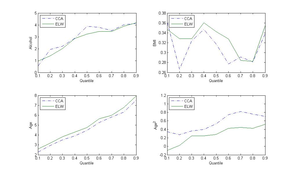 Figure 1
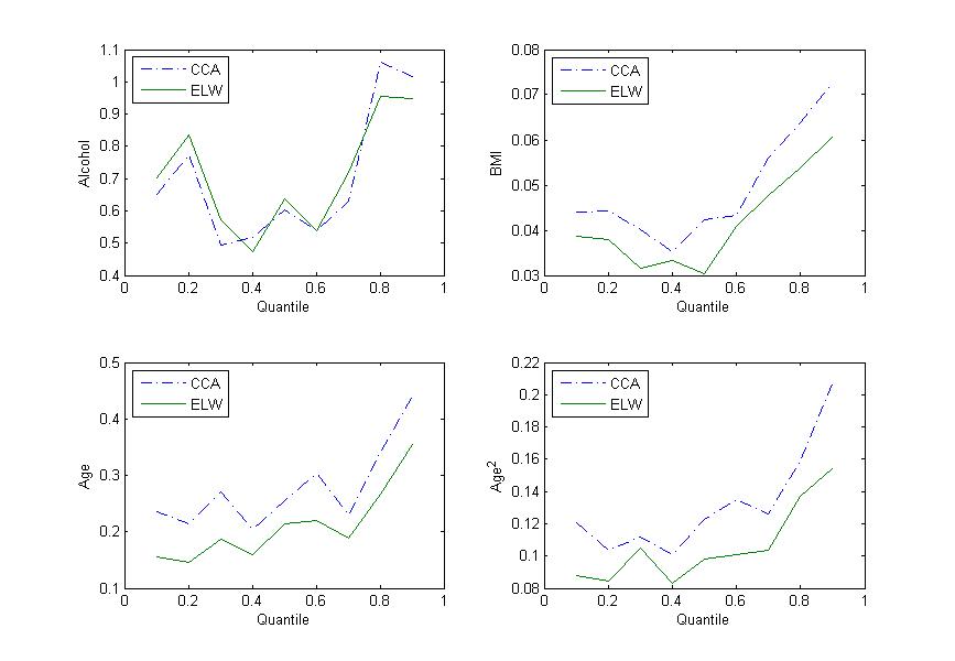 Figure 2
| n | Estimator | ||||
|---|---|---|---|---|---|
| 0.3 | 100 | -0.0022 (0.1185) | 0.0084 (0.1095) | -0.0062 (0.1272) | |
| 0.0072 (0.2403) | 0.0032 (0.1851) | -0.0030 (0.1853) | |||
| -0.1714(0.3065) | 0.0130 (0.2128) | -0.0042 (0.2077) | |||
| -0.1808 (0.3021) | 0.0231 (0.2144) | -0.0120 (0.1945) | |||
| -0.0004 (0.2446) | 0.0107 (0.1875) | -0.0098 (0.1752) | |||
| 300 | 0.0016 (0.0685) | 0.0001 (0.0617) | -0.0014 (0.0676) | ||
| 0.0008 (0.1332) | 0.0032 (0.1031) | -0.0011 (0.1016) | |||
| -0.1669 (0.2188) | 0.0133 (0.1167) | -0.0068 (0.1150) | |||
| -0.1672 (0.2079) | 0.0155 (0.1116) | -0.0097(0.0968) | |||
| -0.0007 (0.1252) | 0.0053 (0.1002) | -0.0032 (0.0873) | |||
| 0.5 | 100 | -0.0021 (0.1128) | 0.0018 (0.0997) | 0.0038 (0.1187) | |
| 0.0016 (0.2347) | 0.0014 (0.1781) | 0.0073 (0.1765) | |||
| -0.1636 (0.2761) | 0.0148 (0.1851) | -0.0020 (0.1850) | |||
| -0.1693 (0.2794) | 0.0209 (0.1814) | -0.0076 (0.1649) | |||
| -0.0023 (0.2326) | 0.0042 (0.1685) | 0.0007 (0.1617) | |||
| 300 | -0.0015 (0.0648) | 0.0002 (0.0608) | 0.0011 (0.0679) | ||
| -0.0001 (0.1274) | 0.0008 (0.0979) | 0.0017 (0.0973) | |||
| -0.1646 (0.2040) | 0.0136 (0.1036) | -0.0073 (0.1003) | |||
| -0.1650 (0.2007) | 0.0158 (0.1002) | -0.0087 (0.0891) | |||
| -0.0017 (0.1238) | 0.0032 (0.0954) | -0.0001 (0.0889) | |||
| 0.7 | 100 | -0.0090 (0.1216) | 0.0025 (0.1147) | 0.0021 (0.1212) | |
| -0.0232 (0.2471) | 0.0118 (0.1864) | -0.0042 (0.1791) | |||
| -0.1750 (0.2839) | 0.0253 (0.1845) | -0.0089 (0.1790) | |||
| -0.1772 (0.2901) | 0.0263 (0.1868) | -0.0105 (0.1694) | |||
| -0.0203 (0.2498) | 0.0076 (0.1870) | 0.0002 (0.1795) | |||
| 300 | -0.0014 (0.0706) | 0.0019 (0.0630) | 0.0001 (0.0708) | ||
| 0.0018 (0.1371) | -0.0032 (0.1008) | 0.0019 (0.1028) | |||
| -0.1576 (0.2007) | 0.0136 (0.1046) | -0.0062 (0.1033) | |||
| -0.1557 (0.1983) | 0.0130 (0.1006) | -0.0059 (0.0935) | |||
| 0.0025 (0.1325) | -0.0003 (0.0969) | 0.0009 (0.0964) |
Peer Reviews
No public reviews on file for this paper yet. If you reviewed it on a platform where reviews are public (OpenReview, ICLR, NeurIPS, ICML), you can paste yours below so the community can read it here.
Videos
No videos yet. Explain this paper in a talk, walkthrough, or lecture? Add one.
Taxonomy
TopicsStatistical Methods and Inference · Statistical Methods and Bayesian Inference · Statistical Distribution Estimation and Applications
Weighted empirical likelihood for quantile regression with nonignorable missing covariates
Xiaohui Yuan
Xiaogang Dong
School of Basic Science, Changchun University of Technology, Changchun 130012, China
Abstract
In this paper, we propose an empirical likelihood-based weighted estimator of regression parameter in quantile regression model with nonignorable missing covariates. The proposed estimator is computationally simple and achieves semiparametric efficiency if the probability of missingness on the fully observed variables is correctly specified. The efficiency gain of the proposed estimator over the complete-case-analysis estimator is quantified theoretically and illustrated via simulation and a real data application.
keywords:
Complete-case-analysis estimator, Empirical likelihood, Nonignorable missing covariates, Quantile regression
††journal:
1 Introduction
Quantile regression, as introduced by Koenker and Bassett (1978), is robust against outliers and can describe the entire conditional distribution of the response variable given the covariates. Due to these advantages, quantile regression became appealing in econometrics, statistics, and biostatistics. The book by Koenker (2005) contains a comprehensive account of overview and discussions in quantile regression.
Let denote the outcome variable, be a vector of covariates which is always observed, and be a vector of covariates which may not be observed for all subjects. The quantile regression model assumes that the -th conditional quantile of given and :
[TABLE]
where and is interior to parameter space , is a compact subset of . We are interested in the inference about based on a random sample of incomplete data
[TABLE]
where all the ’s and ’s are observed, and if is missing, otherwise .
The most commonly used method for handling missing covariate data is the complete-case analysis (CCA), with only the remaining complete data used to perform a regression-based or likelihood-based analysis. The CCA esitmator of is given by
[TABLE]
where is the quantile loss function and is the indicator function.
In statistic literature, there are three missing data categories (Little and Rubin, 2002). The first case is missing completely at random (MCAR), i.e., data missing mechanism is independent of any observable or unobservable quantities. The second case is missing at random (MAR), i.e., data missing mechanism depends on the observed variables. The third case is not missing at random (NMAR) or nonignorable, i.e., data missing mechanism depends on their own values.
When ’s are not MCAR, the CCA estimator can be biased. Consistent and efficient estimators have been proposed in the statistical literature for the quantile regression model when the covariates data are MAR. See for example, Wei et al. (2012) developed an iterative imputation procedure for estimating the conditional quantile in the presence of missing covariates. Sherwood et al. (2013) proposed an inverse probability weighted (IPW) approach to correct for the bias from longitudinal dropouts. Chen et al. (2015) examined the problem of estimation in a quantile regression model and developed three nonparametric methods when observations are missing at random under independent and nonidentically distributed errors. Liu and Yuan (2016) proposed a weighted quantile regression model with weights chosen by empirical likelihood. This approach efficiently incorporates the incomplete data into the data analysis by combining the complete data unbiased estimating equations and incomplete data unbiased estimating equations. However, it may not be an easy task to extend these methods to deal with NMAR missing data mechanisms, because these methods are biased under the NMAR assumption.
NMAR is the most difficult problem in the missing data literature. Following Little and Zhang (2011) and Bartlett et al. (2014), we make the following “not missing at random” (NMAR) assumption:
[TABLE]
The NMAR assumption (3) implies that, missingness in a covariate depends on the value of that covariate, but is conditionally independent of outcome. The CCA estimator is valid but inefficient under the assumption (3) because it fails to draw on the observed information contained in the incomplete cases.
In the context of mean regression model, Bartlett et al. (2014) proposed an augmented CCA estimator to improve upon the efficiency of CCA estimator by modeling an additional model for the probability of missingness on the fully observed variables, i.e. . The estimating function used in Bartlett et al. (2014) utilizes all the observed data by drawing on the information available from both complete and incomplete cases and thus improves upon the efficiency of CCA estimator. Note that under NMAR assumption (3), , whose feasible estimators are not available, since the observations of are missing on some subjects. Thanks to the NMAR assumption (3), there is no need to estimate under the assumption (3). Recently, Xie and Zhang (2017) proposed an empirical likelihood approach for estimating the regression parameters in mean regression model with missing covariates under NMAR assumption (3). They showed that the empirical likelihood estimator can improve estimation efficiency if is correctly specified.
In this paper, we put forward an empirical likelihood-based weighted (ELW) estimator for estimating quantile regression model with nonignorable missing covariates under NMAR assumption (3). To fully utilize the information contained in the incomplete data, we incorporate the unbiased estimating equations of incomplete observations into empirical likelihood and obtain the empirical likelihood-based weights to adjust the CCA estimator defined in (2). The proposed ELW estimator is computationally simple as the CCA estimator and achieves semiparametric efficiency if is correctly specified.
Empirical likelihood is an effective approach to improving efficiency. For a comprehensive review of the empirical likelihood method, one can refer to Qin and Lawless (1994), Owen (2001), Lopez et al. (2009) among others. For applications of empirical likelihood in missing-data problems, one can refer to Wang and Rao (2002), Qin et al. (2009), Liu and Yuan (2012), Liu et al. (2013), Zhong and Qin (2017) among others.
The rest of this paper is organized as follows. In section 2, we introduce the empirical likelihood-based weighted estimator for quantile regression model. In section 3, we show that the ELW estimator is asymptotically equivalent to the profile empirical likelihood estimator and thus achieves semiparametric efficiency. Numerical studies are reported in sections 4-5. Proofs of the main theorems needed are given in the Appendix.
2 The empirical likelihood-based weighted estimation
In this section, we propose the ELW estimator of under the assumption (3). Under the assumption (3), we only need to estimate the probability of being observed given and , i.e. . Following Bartlett et al. (2014) and Xie and Zhang (2017), we assume that is described by the probability model:
[TABLE]
where is a unknown vector parameter. It is natural to estimate by the binomial likelihood estimator which maximizes the binomial log-likelihood
[TABLE]
Let be a working model of with . In the following, we proposed the ELW estimator of . Define
[TABLE]
Let represent the probability weight allocated to , where and is a consistent estimator for some . If is correctly specified, one can show that , where . Then, we maximize the empirical likelihood function subject to the constraints:
[TABLE]
By using the Lagrange multiplier method, we get
[TABLE]
where is the Lagrange multiplier that satisfies
[TABLE]
The ELW estimator of is given by
[TABLE]
Define
[TABLE]
From (2), it is easily seen . For fixed , solving (7) is a well-behaved optimization problem since the objective function is globally concave and can be solved by a simple Newton-Raphson numerical procedure.
Let and denote respectively the conditional distribution and density functions of given . Denote
[TABLE]
The following regularity conditions help us in doing asymptotic analysis:
- C1
The -th conditional quantile of given is and has a bounded support. 2. C2
. 3. C3
, , are positive definite. 4. C4
is absolutely continuous and is uniformly bounded away from 0 and at 0. 5. C5
(a) (b) for some (c) For all , admits all third partial derivatives for all in a neighborhood of the true value , \biggr{\|}\frac{\partial^{3}\pi(Y_{i},Z_{i},\gamma)}{\partial\gamma_{k}\partial\gamma_{l}\partial\gamma_{m}}\biggr{\|} and are bounded by an integrable function for all in this neighborhood. 6. C6
For all , admits all second partial derivatives and for all and in a neighborhood of . , and are bounded by an integrable function for all and in this neighborhood.
The asymptotic distribution of is given by the following theorem.
Theorem 2.1
Under conditions C1-C4, as , where
The asymptotic distribution of is given by the following theorem.
Theorem 2.2
Under conditions C1-C6, as , where
[TABLE]
* and *
For two matrices and , we write if is a nonnegative-definite matrix.
Corollary 2.3
If both and are positive definite, we have , and the equality holds if and only if .
Corollary 2.3 reveals that is at least as efficient as for any working regression function , whether or not it correctly identifies the optimal regression function .
Although can be obtained easily, it is difficult to estimate the limiting covariance matrix analytically. We apply the resampling method in Liu and Yuan (2016) to the inference about .
3 Simulation studies
In this section, we investigate the performance of the proposed estimator and several other estimators based on Monte-Carlo simulations.
The simulated data are generated by the procedure of Bartlett et al. (2014), in which the non-missing indicator is distributed with , and is generated from a trivariate normal distribution conditional on :
[TABLE]
where , , and .
It is easy to verify that the assumption is satisfied in this setup. Conditional on and , the probability of is a logistic regression with
[TABLE]
where and . The conditional quantile model of interest is specified as
[TABLE]
with , , .
We set , and generate 1000 Monte Carlo data sets of sample sizes and . Five estimators are considered:
: the quantile regression estimator with the full observations. This is the ideal case, but it is not feasible in practice. Nevertheless, we used it as a benchmark for comparison; 2. 2.
: the CCA estimator defined in equation (2); 3. 3.
: the IPW estimator assuming MAR, introduced in Sherwood et al. (2013); 4. 4.
: the ELW estimator assuming MAR, proposed by Liu and Yuan (2016); 5. 5.
: the ELW estimator defined in equation (6).
The empirical bias and the root-mean-squared errors (RMSEs) of the proposed estimators with sample sizes of 100 and 300 are reported in Table 1. The results can be summarized as follows: the CCA estimator and the ELW estimator are unbiased as expected. While and for are clearly biased. performs better than in terms of RMSE in most cases, which agrees with our theory. and are improved in terms of RMSE as the sample size goes up from 100 to 300.
4 Data analysis
In this section, we apply the proposed method to the data on alcohol consumption, age, body mass index and systolic blood pressure from the 2013-2014 NHANES. We model the population quantile of SBP (systolic blood pressure) as a function of the following four covariates: BMI (body mass index), Alcohol (log{alcohol consumption per day}), Age () and Age2 ().
In our analysis, there are 7104 observations in the data set, where the dependent variable SBP and the covariates BMI and Age have complete data, the covariate Alcohol are missing 53.29%. It is a priori plausible that missingness in Alcohol is primarily dependent on the value of itself (i.e. MNAR), and that missingness in Alcohol is independent of SBP conditional on Alcohol, BMI, Age, and Age2. Consequently, CCA is expected to give valid inferences, while the MAR assumption likely does not hold.
For , let denote the th observation of SBP, denote the th observation of =(BMI, Age, Age2)T and denote the th observation of Alcohol. Then, we consider the following model for the th conditional quantile of given :
[TABLE]
where and . We consider two estimators and . For the ELW method, the probability of whether the Alcohol is observed is modeled by .
In Figure 1, we plot the estimated regression coefficients, and for , , and , at quantile levels . We see that the CCA and ELW methods produce similar estimated regression coefficients. In Figure 2, we plot the standard errors of and for , , and at various quantile levels. The standard error of is smaller than that of in most cases.
5 Conclusions
In this paper, we develop weighted empirical likelihood approach for estimating the conditional quantile functions in linear models with nonignorable missing covariates. By incorporating the unbiased estimating equations of incomplete data into empirical likelihood, the ELW estimator can achieve semiparametric efficiency if the probability of missingness is correctly specified. We will extend the proposed methods to other regression models, which will be investigated in the future work.
Acknowledgements
Xiaohui Yuan was partly supported by the NSFC (No.11401048, 11671054,11701043). Xiaogang Dong was partly supported by the NSFC (No. 11571051).
6 Appendix
In the section, we list a preliminary lemma which has been used in the proofs of the main results in section 2.
Lemma 6.1
Under conditions C1-C5, we have
[TABLE]
where is defined in (7).
**The proof of Lemma 6.1 ** By Lemma A.2 in Liu and Yuan (2016), we have
[TABLE]
where . By a Taylor expansion,
[TABLE]
where is a point on the segment connecting and . By the law of large numbers, we have
[TABLE]
By the asymptotic properties of maximum likelihood estimate, we have
[TABLE]
[TABLE]
The desired result follows.
**The proof of Theorem 2.1 ** The proof is similar to the proof of Theorem 4.1 in Koenker (2005, page 120).
** The proof of Theorem 2.2 ** For , let
[TABLE]
where . The function is convex and is minimized at . Following Knight’s identity (Knight,1998)
[TABLE]
we can write where
[TABLE]
We first give the asymptotic expression of (12). Applying a Taylor expansion, we get
[TABLE]
By the law of large numbers, we have
[TABLE]
By Lemma 6.1,
[TABLE]
where .
Next, we give the asymptotic expression of (13). A Taylor expansion reveals that
[TABLE]
Moreover, similar to the proof of Theorem 4.1 in Koenker(2005), one can show that
[TABLE]
Thus, we only need to show that is asymptotically negligible. By Lemma 6.1 and Lemma D.2 in Kitamura et al. (2004), we have and . Then,
[TABLE]
By the asymptotic expressions of (12) and (13), we conclude that , where
[TABLE]
Then, it follows that
[TABLE]
where
[TABLE]
Furthermore, by simple algebra, one can verify that
[TABLE]
and
[TABLE]
Therefore,
[TABLE]
Let
[TABLE]
One can write as . It is easily verified that
[TABLE]
and
[TABLE]
Thus,
[TABLE]
The desired result follows by the central limit theorem.
** The proof of Theorem LABEL:el ** According to the proof of Theorem 1 of Lopez et al.(2009), it can be shown that
[TABLE]
where , S_{1}=\left(\begin{array}[]{cc}F_{\beta}&0\\ 0&D_{2}\\ 0&S_{B}\end{array}\right) and S_{2}=\left(\begin{array}[]{ccc}S_{\phi}&D_{3}&D_{4}\\ D_{3}^{T}&D_{1}&D_{2}\\ D_{4}^{T}&D_{2}^{T}&S_{B}\end{array}\right).
Let E_{22}=\left(\begin{array}[]{cc}D_{1}&D_{2}\\ D_{2}^{T}&S_{B}\end{array}\right), then we write S_{2}=\left(\begin{array}[]{cc}S_{\phi}&F_{g}\\ F_{g}^{T}&E_{22}\end{array}\right), where is defined in (14) We know that
[TABLE]
with . Note that can be written as
[TABLE]
where , , and . Therefore, we have
[TABLE]
where By direct calculation, it follows that
[TABLE]
and The desired result follows.
Reference
The reference list from the paper itself. Each links out to its DOI / PubMed record.
- 1(1) Bartlett J W, Carpenter J R, Tilling K, et al. 2014. Improving upon the efficiency of complete case analysis when covariates are MNAR[J]. Biostatistics, 15(4): 719-730.
- 2(2) Chen X, Wan A T K, Zhou Y. 2015. Efficient quantile regression analysis with missing observations[J]. Journal of the American Statistical Association, 110(510):00-00.
- 3(3) Kitamura Y, Tripathi G, Ahn H. 2004. Empirical likelihood-based inference in conditional moment restriction Models[J]. Econometrica, 72(6): 1667-1714.
- 4(4) Knight K. 1998. Limiting distributions for L 1 subscript 𝐿 1 L_{1} regression estimators under general conditions[J]. Annals of Statistics, 26: 755-770.
- 5(5) Koenker, R. and Bassett, G. 1978. Regression quantiles. Econometrica,46, 33-50.
- 6(6) Koenker R. 2005. Quantile regression[M]. Cambridge university press.
- 7(7) Little RJA, Rubin DB 2002 Statistical analysis with missing data, 2nd ed, Wiley, Hoboken, NJ.
- 8(8) Little, R.J., Zhang, N. 2011. Subsample ignorable likelihood for regression analysis with missing data. J R Stat Soc Ser C 60: 591-605.